Humpback whale – Geospatial Ecology of Marine Megafauna Laboratory

Announcing our new project: SLATE – Scar-based Long-term Assessment of Trends in whale Entanglements

By Solène Derville, Postdoc, OSU Department of Fisheries, Wildlife, and Conservation Science, Geospatial Ecology of Marine Megafauna Lab

Filling the gaps

Reports of whale entanglements have been on the rise over the last decade on the US West Coast, with Dungeness crab fishing gear implicated in many cases (Feist et al., 2021; Samhouri et al., 2021; Santora et al., 2020). State agencies are responsible for managing this environmental issue that has implications both for the endangered whale sub-populations that are subject to entanglements, and for the fishing activities, which play an important social, cultural, and economic role for coastal communities. In Oregon, the Oregon Whale Entanglement Working Group (today the Oregon Entanglement Advisory Committee, facilitated by ODFW – Oregon Department of Fish and Wildlife) formed in 2017, tasked with developing options to reduce entanglement risk. The group members composed of managers, researchers and fishermen identified that a lack of information and understanding of whale distribution in Oregon waters was a significant knowledge gap of high priority.

In response, the GEMM Lab and its collaborators at ODFW developed the OPAL project (Overlap Predictions About Large whales, phase 1: 2018-2022). The first phase of the project (phase 1) was developed to 1) model and predict large whale distribution off the coast of Oregon in relation to dynamic environmental conditions, and 2) assess overlap with commercial crab fishing gear to inform conservation efforts. Although this first phase was extended up to June as a result of COVID, it is now coming to an end. As a postdoc in the GEMM Lab, I have been the main analyst working on this project. The habitat use models that I generated from several years of aerial and boat-based surveys provide improved knowledge about where and when rorqual whales (combining blue, humpback and fin) are most abundant (Derville et al., 2022). Moreover, we are about to publish an analysis of overlap between whale predicted densities and commercial Dungeness crab fishing effort. This analysis of co-occurrence over 10 years shows distinct spatio-temporal patterns in relation to climatic fluctuations affecting the northern California Current System (Derville et al., In review).

Although we are quite satisfied with the outputs of these four years of research, this is not the end of it! Project OPAL continues into a second phase (2022-2025; supported by NOAA Section 6 funding), during which models will be improved and refined via incorporation of new survey data (helicopter and boat-based) as well as prey data (krill and fish distribution). PhD student Rachel Kaplan is a key contributor to this research, and I will do my best to keep assisting her in this journey in the years to come.

Announcing SLATE!

As this newly acquired knowledge leads to potentially new management measures in Oregon, it becomes essential for managers to evaluate their impacts on the entanglement issue. But how do we know exactly how many entanglements occur during any year within Oregon waters? Is recording reports of entanglements or signs of entanglements in stranded whales enough? The simple answer is no. Entanglements are notoriously under-detected and under-reported (Tackaberry et al., 2022). Over the US West Coast, entanglements are also relatively rare events that can easily go unnoticed in the immensity of the ocean. Moreover, entangled large whales are often able to carry the fishing gear for some time away from the initial gearset location, which makes it hard to locate the origin of the gear causing problems (van der Hoop et al., 2017).

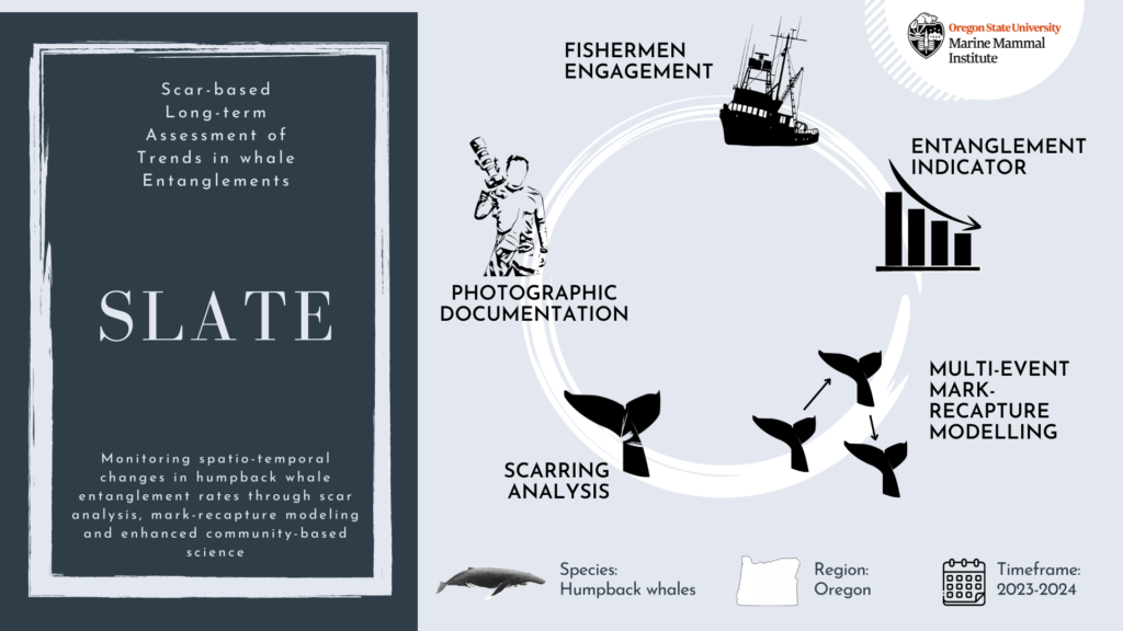
**Figure 1:** Graphical representation of the SLATE project representing the different tasks described below. Work in progress…

Our approach to the challenge of assessing humpback whale entanglement rates in Oregon waters is to use scar analysis. Our new “SLATE” (Scar-based Long-term Assessment of Trends in whale Entanglements, Figure 1) project will be using scar-based methods as a proxy to detect unobserved entanglement events (e.g., Basran et al., 2019; Bradford et al., 2009; George et al., 2017; Knowlton et al., 2012; Robbins, 2012). Indeed, this approach has been effective to detect potential interactions with fishing gear at a much higher frequency than entanglement reports in the Atlantic Ocean (e.g., only 10% of entanglements of humpback whales in the Gulf of Maine were estimated to be reported; Robbins, 2012). We will be examining hundreds of photographs of humpback whales observed in Oregon waters to try to detect wrapping scars and notches that result from entanglement events. Based on this scar pattern, we will assign each whale a qualitative probability of prior entanglement (i.e., uncertain, low, high). We will specifically be looking at the caudal peduncle (the attachment point of the whale’s fluke, see Figure 2) following a methodology developed in the Gulf of Maine by Robbins & Mattila, (2001).

**Figure 2:** Examples of unhealed injuries interpreted as entanglement related in 2010 in the Gulf of Maine. Figure reproduced from (Robbins, 2012).

Data please?

While this approach is to-date the most applicable way to assess otherwise undetected entanglements, it is sometimes limited by sample size. Although we plan to collect more photos in the field in summer 2023 and 2024, this long-term analysis of scarring patterns would not be possible without the contribution of the Cascadia Research Collective (CRC) led by John Calambokidis. The CRC humpback whale catalogue will be crucial to assessing entanglement rates at the individual level over the last decade.

Moreover, as we have been contemplating the task ahead of us, we realized that the data collected through traditional scientific surveys might not be sufficient to achieve our goal. We need the help of the people who live off the ocean and encounter whales on a day-to-day basis: fishermen. That is why we decided to solicit interested fishermen to take photographs of whales while at sea. Starting this year, we will work with at least three self-selected fishermen who are interested in supporting this program and collecting data to support the research efforts. Participants will be provided a stipend, equipped with a high-quality camera, and trained to photograph whales while following National Oceanic and Atmospheric Administration (NOAA) Marine Mammal Protection Act (MMPA) guidelines.

And here come the statistics…

If we have some of my previous blogs (e.g., May 2022, June 2018), you know that I usually participate in projects that have a significant statistical modeling component. As part of the SLATE project, I will be trying out some new approaches that I never had the opportunity to work with before, which makes me feels both super excited and slightly apprehensive!

First, I will analyze humpback whale scarring at the population level. That means I will be using all available photos of whales in Oregon waters without considering individual identification, and I will model the probability of entanglement scars in relation to space and time. This model will help us answer questions such as: did whales have a higher chance of becoming entangled in certain years over others? Did whales observed in a certain zone in Oregon waters have a higher risk of getting entangled?

Second, I will analyze humpback whale scarring at the individual level. This time, we will only use encounters of a selected number of individuals that have a long recapture history, meaning that they were photo-identified and resighted several times throughout the last decade. Using a genetic database produced by the Cetacean Conservation and Genomic Laboratory (CCGL, Marine Mammal Institute), we will also be able to tell to which “Distinct Population Segment” (DPS) some of these individual whales belong. Down the line, this is an important piece of information because humpback whale DPS do not breed in the same areas, and these groups have different levels of population health. Then, we will use what is known as a “multi-event mark-recapture model” to estimate the probability of entanglement as a function of time and spatial residency or DPS assignment, while accounting for detection probability and survival.

Through these analyses, our goal is to produce a single indicator to help managers assess the effects of mandatory or voluntary changes in Oregon fishing practices. In the end, we hope that these models will provide a measurable and robust way of monitoring whale entanglements in fishing gear off the coast of Oregon.

References

Basran, C. J., Bertulli, C. G., Cecchetti, A., Rasmussen, M. H., Whittaker, M., & Robbins, J. (2019). First estimates of entanglement rate of humpback whales Megaptera novaeangliae observed in coastal Icelandic waters. Endangered Species Research, 38(February), 67–77. https://doi.org/10.3354/ESR00936

Bradford, A. L., Weller, D. W., Ivashchenko, Y. v., Burdin, A. M., & Brownell, R. L. (2009). Anthropogenic scarring of western gray whales (Eschrichtius robustus). Marine Mammal Science, 25(1), 161–175. https://doi.org/10.1111/j.1748-7692.2008.00253.x

Derville, S., Barlow, D. R., Hayslip, C. E., & Torres, L. G. (2022). Seasonal, Annual, and Decadal Distribution of Three Rorqual Whale Species Relative to Dynamic Ocean Conditions Off Oregon, USA. Frontiers in Marine Science, 9, 1–19. https://doi.org/10.3389/fmars.2022.868566

Derville, S., Buell, T., Corbett, K., Hayslip, C., & Torres, L. G. (n.d.). Exposure of whales to entanglement risk in Dungeness crab fish-ing gear in Oregon, USA, reveals distinctive spatio-temporal and climatic patterns. Biological Conservation.

Feist, B. E., Samhouri, J. F., Forney, K. A., & Saez, L. E. (2021). Footprints of fixed-gear fisheries in relation to rising whale entanglements on the U.S. West Coast. Fisheries Management and Ecology, 28(3), 283–294. https://doi.org/10.1111/fme.12478

George, J. C., Sheffield, G., Reed, D. J., Tudor, B., Stimmelmayr, R., Person, B. T., Sformo, T., & Suydam, R. (2017). Frequency of injuries from line entanglements, killer whales, and ship strikes on bering-chukchi-beaufort seas bowhead whales. Arctic, 70(1), 37–46. https://doi.org/10.14430/arctic4631

Knowlton, A. R., Hamilton, P. K., Marx, M. K., Pettis, H. M., & Kraus, S. D. (2012). Monitoring North Atlantic right whale Eubalaena glacialis entanglement rates: A 30 yr retrospective. Marine Ecology Progress Series, 466(Kraus 1990), 293–302. https://doi.org/10.3354/meps09923

Robbins, J. (2012). Scar-Based Inference Into Gulf of Maine Humpback Whale Entanglement : 2010 (Issue January). Report to the Northeast Fisheries Science Center National Marine Fisheries Service, EA133F09CN0253 Item 0003AB, Task 3.

Robbins, J., & Mattila, D. K. (2001). Monitoring entanglements of humpback whales ( Megaptera novaeangliae ) in the Gulf of Maine on the basis of caudal peduncle scarring. SC/53/NAH25. Report to the Scientific Committee of the International Whaling Commission, 14, 1–12. http://www.ccbaymonitor.org/pdf/scarring.pdf

Samhouri, J. F., Feist, B. E., Fisher, M. C., Liu, O., Woodman, S. M., Abrahms, B., Forney, K. A., Hazen, E. L., Lawson, D., Redfern, J., & Saez, L. E. (2021). Marine heatwave challenges solutions to human-wildlife conflict. Proceedings of the Royal Society B: Biological Sciences, 288, 20211607. https://doi.org/10.1098/rspb.2021.1607

Santora, J. A., Mantua, N. J., Schroeder, I. D., Field, J. C., Hazen, E. L., Bograd, S. J., Sydeman, W. J., Wells, B. K., Calambokidis, J., Saez, L., Lawson, D., & Forney, K. A. (2020). Habitat compression and ecosystem shifts as potential links between marine heatwave and record whale entanglements. Nature Communications, 11, 536. https://doi.org/10.1038/s41467-019-14215-w

Tackaberry, J., Dobson, E., Flynn, K., Cheeseman, T., Calambokidis, J., & Wade, P. R. (2022). Low Resighting Rate of Entangled Humpback Whales Within the California , Oregon , and Washington Region Based on Photo-Identification and Long-Term Life History Data. Frontiers in Marine Science, 8(January), 1–13. https://doi.org/10.3389/fmars.2021.779448

van der Hoop, J., Corkeron, P., & Moore, M. (2017). Entanglement is a costly life-history stage in large whales. Ecology and Evolution, 7(1), 92–106. https://doi.org/10.1002/ece3.2615

Hope lies in cooperation: the story of a happy whale!

By Solène Derville, Postdoc, OSU Department of Fisheries, Wildlife, and Conservation Science, Geospatial Ecology of Marine Megafauna Lab

I wrote my last blogpost in the midst of winter and feeling overwhelmed as I was trying to fly to the US at the peak of the omicron pandemic… Since then, morale has improved exponentially. I have spent two months in the company of my delightful GEMM lab friends, nerding over statistics, sharing scientific conversations, drinking (good!) beer and enjoying the company of this great group of people. During that stay, I was able to focus on my OPAL project more than I have ever been able to, as I set myself the goal of not getting distracted by anything else during my stay in Newport.

The only one distraction that I do not regret is a post I read one morning on the Cetal Fauna Facebook page, a group of cetacean experts and lovers who share news, opinions, photos… anything cetacean related! Someone was posting a photo of a humpback whale stranded in the 1990s’ on Coolum beach, on the east coast of Australia, which is known as a major humpback whale migratory corridor. The story said that (probably with considerable effort) the whale was refloated by many different individuals and organizations present at the beach on that day, specifically Sea World Research, Rescue & Conservation.

I felt very touched by this story and the photo that illustrated it (Figure 1). Seeing all these people come together in this risky operation to save this sea giant is quite something. And the fact that they succeeded was even more impressive! Indeed, baleen whales strand less commonly than toothed whales but their chances of survival when they do so are minimal. In addition to the actual potential damages that might have caused the whale to strand in the first place (entanglements, collisions, diseases etc.), the beaching itself is likely to hurt the animal in a permanent way as their body collapses under their own weight usually causing a cardiovascular failure (e.g., Fernández et al., 2005)⁠. The rescue of baleen whales is also simply impaired by the sheer size and weight of these animals. Compared to smaller toothed whales such as pilot whales and false killer whales that happen to strand quite frequently over some coastlines, baleen whales are almost impossible to move off the beach and getting close to them when beached can be very dangerous for responders. For these reasons, I found very few reports and publications mentioning successful rescues of beached baleen whales (e.g., Priddel and Wheeler, 1997; Neves et al., 2020).⁠

Figure 1: Stranded humpback whale on Coolum Beach, East Australia, in 1996. Look at the size of the fluke compared to the men who are trying to rescue her! Luckily, that risky operation ended well. This image won Australian Time Magazine Cover of the year. Credit: Sea World Research, Rescue and Conservation. Photo posted by P. Garbett on *https://www.facebook.com/groups/CetalFauna* *– February 26, 2022)*

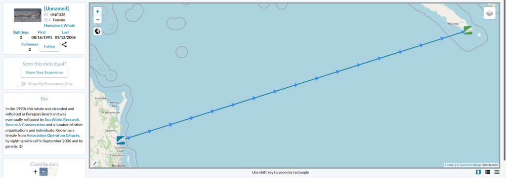
Now the story gets even better… the following day I received an email from Ted Cheeseman, director and co-founder of Happywhale, a collaborative citizen science tool to share and match photographes of cetaceans (initially only humpback whales but has extended to other species) to recognize individuals based on the unique patterns of the their fluke or dorsal fin. The fluke of the whale stranded in Australia in 1991 had one and only match within the Happywhale immense dataset… and that match was to a whale seen in New Caledonia (Figure 2). “HNC338” was the one!

Figure 2: Happy whale page showing the match of HNC338 between East Australia and New Caledonia. https://happywhale.com/individual/78069;enc=284364?fbclid=IwAR1QEG_6JkpH_k2UrF-qp-9qrOboHYakKjlTj0lLbDFygjN5JugkkKVeMQw

Since I conducted my PhD on humpback whale spatial ecology in New Caledonia, I have continued working on a number of topics along with my former PhD supervisor, Dr Claire Garrigue, in New Caledonia. Although I do not remember each and every whale from her catalogue (composed of more than 1600 humpback whales as of today), I do love a good “whale tale” and I was eager to know who this HNC338 was. I quickly looked into Claire’s humpback whale database and sure enough I found it there: encountered at the end of the 2006 breeding season on September 12^th, at a position of 22°26.283’S and 167°01.991’E and followed for an hour. Field notes reported a shy animal that kept the boat at a distance. But most of all, HNC338 was genetically identified as a female and was accompanied by a calf during that season! The calf was particularly big, as expected at this time of the season. What an inspiring thing to think that this whale, stranded in 1996, was resighted 10 years later in a neighboring breeding ground, apparently healthy and raising a calf of her own.

As genetic paternity analysis have been conducted on many New Caledonia calf biopsy samples as part of the Sexy Singing project conducted with our colleagues from St Andrews University in Scotland, we might be able to identify the calf’s father in this breeding stock. Thanks to the great amount of data shared and collected through Happywhale, we are discovering more and more about whale migratory patterns and behavior. It might as well be that this calf’s father was one of those whales that seem to roam over several different breeding grounds (New Caledonia and East Australia). This story is far from finished…

Figure 3: A (pretty bad!) photo of HNC338’s fluke. Luckily the Happywhale matching algorithm is very efficient and was able to detect the similarities of the fluke’s trailing edge compared to figure 1 (Cheeseman et al., 2021)⁠. Also of note, see that small dorsal fin popping out of the waters behind big mama’s fluke? That’s her calf!

From the people who pulled this whale back into the water in 1996, to the scientists and cetacean enthusiasts who shared their data and whale photos online, this story once again shows us that hope lies in cooperation! Happywhale was only created in 2015 but since then it has brought together the general public and the scientists to contribute over 465,000 photos allowing the identification of 75,000 different individuals around the globe. In New Caledonia, in Oregon and elsewhere, I hope that these collective initiatives grow more and more in the future, to the benefit of biodiversity and people.

Did you enjoy this blog? Want to learn more about marine life, research, and conservation? Subscribe to our blog and get weekly updates and more! Just add your name into the subscribe box on the left panel.

References

Cheeseman, T., Southerland, K., Park, J., Olio, M., Flynn, K., Calambokidis, J., et al. (2021). Advanced image recognition: a fully automated, high-accuracy photo-identification matching system for humpback whales. Mamm. Biol. doi:10.1007/s42991-021-00180-9.

Fernández, A., Edwards, J. F., Rodríguez, F., Espinosa De Los Monteros, A., Herráez, P., Castro, P., et al. (2005). “Gas and fat embolic syndrome” involving a mass stranding of beaked whales (Family Ziphiidae) exposed to anthropogenic sonar signals. Vet. Pathol. 42, 446–457. doi:10.1354/vp.42-4-446.

Neves, M. C., Neto, H. G., Cypriano-Souza, A. L., da Silva, B. M. G., de Souza, S. P., Marcondes, M. C. C., et al. (2020). Humpback whale (megaptera novaeangliae) resighted eight years after stranding. Aquat. Mamm. 46, 483–487. doi:10.1578/AM.46.5.2020.483.

Priddel, D., and Wheeler, R. (1997). Rescue of a Bryde’s whale Balaenoptera edeni entrapped in the Manning River, New South Wales: Unmitigated success or unwarranted intervention? Aust. Zool. 30, 261–271. doi:10.7882/AZ.1997.002.

What makes a good meal for a hungry whale?

By Dawn Barlow, PhD student, OSU Department of Fisheries and Wildlife, Geospatial Ecology of Marine Megafauna Lab

In the vast and dynamic marine environment, food is notoriously patchy and ephemeral [1]. Predators such as marine mammals and seabirds must make a living in this dynamic environment by locating and capturing those prey patches. Baleen whales such as blue and humpback whales have a feeding strategy called “lunge feeding”, whereby they accelerate forward and open their massive jaws, engulf prey-laden water in their buccal pouch that expands like an accordion, and filter the water out through baleen plates so that they are left with a mouthful of food (Fig. 1) [2]. This approach is only efficient if whales can locate and target dense prey patches that compensate for the energetic costs of diving and lunging [3]. Therefore, not only do these large predators need to locate enough food to survive in the expansive and ever-changing ocean, they need to locate food that is dense enough to feed on, otherwise they actually lose more energy by lunging than they gain from the prey they engulf.

**Figure 1.** Schematic of a humpback whale lunge feeding on a school of fish. Illustration by Alex Boersma.

Why do baleen whales rely on such a costly feeding approach? Interestingly, this tactic emerged after the evolution of schooling behavior of prey such as zooplankton and forage fish (e.g., herring, anchovy, sand lance) [4]. Only because the prey aggregate in dense patches can these large predators take advantage of them by lunge feeding, and by engulfing a whole large patch they efficiently exploit these prey patches. Off the coast of California, where krill aggregations are denser in deeper water, blue whales regularly dive to depths of 100-300 m in order to access the densest krill patches and get the most bang for their buck with every lunge [5]. In New Zealand, we have found that blue whales exploit the dense krill patches near the surface to maximize their energetic gain [6], and have documented a blue whale bypassing smaller krill patches that presumably were not worth the effort to feed on.

By now hopefully I have convinced you of the importance of dense prey patches to large whales looking for a meal. It is not necessarily only a matter of total prey biomass in an area that is important to a whale, it is whether that prey biomass is densely aggregated. What makes for a dense prey patch? Recent work has shown that forage species, namely krill and anchovies, swarm in response to coastal upwelling [7]. While upwelling events do not necessarily change the total biomass of prey available to a whale over a spatial area, they may aggregate prey to a critical density to where feeding by predators becomes worthwhile. Forage species like zooplankton and small fish may school because of enhanced food resources, for predator avoidance, or reproductive grouping. While the exact behavioral reason for the aggregation of prey may still only be partially understood, the existence of these dense patches allows the largest animals on the planet to survive.

Another big question is, how do whales actually find their food? In the vast, seemingly featureless, and ever-changing ocean environment, how does a whale know where to find a meal, and how do they know it will be worthwhile before they take a lunge? In a review paper written by GEMM Lab PI Dr. Leigh Torres, she suggests it is all a matter of scale [8]. On a very large scale, baleen whales likely rely on oceanographic stimuli to home in on areas where prey are more likely to be found. Additionally, recent work has demonstrated that migrating blue whales return to areas where foraging conditions were best in previous years, indicating a reliance on memory [9,10]. On a very fine scale, visual cues may inform how a blue whale chooses to lunge [6,8,11].

What does it matter what a blue whale’s favorite type of meal is? Besides my interest in foundational research in ecology such as predator-prey dynamics, these questions are fundamental to developing effective management approaches for reducing impacts of human activities on whales. In the first chapter of my PhD, I examined how oceanographic features of the water column structure krill aggregations, and how blue whale distribution is influenced by oceanography and krill availability [12]. Currently, I am deep into my second chapter, analyzing the pathway from wind to upwelling to krill to blue whales in order to better understand the links and time lags between each step. Understanding the time lags will allow us to make more informed models to forecast blue whale distribution in my third chapter. Environmental managers in New Zealand plan to establish a protected area to conserve the population of blue whales that I study [13] on their foraging grounds. Understanding where blue whales will be distributed, and consequently how their distribution patterns might shift with environmental conditions or overlap with human activities, comes down the fundamental question I started this blog post with: What makes a good meal for a hungry whale?

References

1. Hyrenbach KD, Forney KA, Dayton PK. 2000 Marine protected areas and ocean basin management. Aquat. Conserv. Mar. Freshw. Ecosyst. 10, 437–458. (doi:10.1002/1099-0755(200011/12)10:6<437::AID-AQC425>3.0.CO;2-Q)

2. Goldbogen JA, Cade DE, Calambokidis J, Friedlaender AS, Potvin J, Segre PS, Werth AJ. 2017 How Baleen Whales Feed: The Biomechanics of Engulfment and Filtration. Ann. Rev. Mar. Sci. 9, 367–386. (doi:10.1146/annurev-marine-122414-033905)

3. Goldbogen JA, Calambokidis J, Oleson E, Potvin J, Pyenson ND, Schorr G, Shadwick RE. 2011 Mechanics, hydrodynamics and energetics of blue whale lunge feeding: efficiency dependence on krill density. J. Exp. Biol. 214, 131–146. (doi:10.1242/jeb.048157)

4. Cade DE, Carey N, Domenici P, Potvin J, Goldbogen JA. 2020 Predator-informed looming stimulus experiments reveal how large filter feeding whales capture highly maneuverable forage fish. Proc. Natl. Acad. Sci. U. S. A. (doi:10.1073/pnas.1911099116)

5. Hazen EL, Friedlaender AS, Goldbogen JA. 2015 Blue whales (Balaenoptera musculus) optimize foraging efficiency by balancing oxygen use and energy gain as a function of prey density. Sci. Adv. 1, e1500469–e1500469. (doi:10.1126/sciadv.1500469)

6. Torres LG, Barlow DR, Chandler TE, Burnett JD. 2020 Insight into the kinematics of blue whale surface foraging through drone observations and prey data. PeerJ (doi:10.7717/peerj.8906)

7. Benoit-Bird KJ, Waluk CM, Ryan JP. 2019 Forage Species Swarm in Response to Coastal Upwelling. Geophys. Res. Lett. 46, 1537–1546. (doi:10.1029/2018GL081603)

8. Torres LG. 2017 A sense of scale: Foraging cetaceans’ use of scale-dependent multimodal sensory systems. Mar. Mammal Sci. 33, 1170–1193. (doi:10.1111/mms.12426)

9. Abrahms B et al. 2019 Memory and resource tracking drive blue whale migrations. Proc. Natl. Acad. Sci. U. S. A. (doi:10.1073/pnas.1819031116)

10. Szesciorka AR, Ballance LT, Širovi A, Rice A, Ohman MD, Hildebrand JA, Franks PJS. 2020 Timing is everything: Drivers of interannual variability in blue whale migration. Sci. Rep. 10, 1–9. (doi:10.1038/s41598-020-64855-y)

11. Friedlaender AS, Herbert-Read JE, Hazen EL, Cade DE, Calambokidis J, Southall BL, Stimpert AK, Goldbogen JA. 2017 Context-dependent lateralized feeding strategies in blue whales. Curr. Biol. (doi:10.1016/j.cub.2017.10.023)

12. Barlow DR, Bernard KS, Escobar-Flores P, Palacios DM, Torres LG. 2020 Links in the trophic chain: Modeling functional relationships between in situ oceanography, krill, and blue whale distribution under different oceanographic regimes. Mar. Ecol. Prog. Ser. (doi:https://doi.org/10.3354/meps13339)

13. Barlow DR et al. 2018 Documentation of a New Zealand blue whale population based on multiple lines of evidence. Endanger. Species Res. 36, 27–40. (doi:https://doi.org/10.3354/esr00891)

Marine heatwaves and their impact on marine mammals

By Dawn Barlow, PhD student, OSU Department of Fisheries and Wildlife, Geospatial Ecology of Marine Megafauna Lab

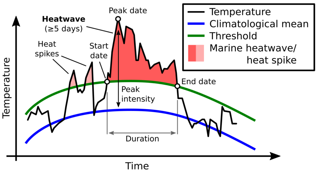
In recent years, anomalously warm ocean temperatures known as “marine heatwaves” have sparked considerable attention and concern around the world. Marine heatwaves (MHW) occur when seawater temperatures rise above a seasonal threshold (greater than the 90^th percentile) for five consecutive days or longer (Hobday et al. 2016; Fig. 1). With global ocean temperatures continuing to rise, we are likely to see more frequent and more intense MHW conditions in the future. Indeed, the global prevalence of MHWs is increasing, with a 34% rise in frequency, a 17% increase in duration, and a 54% increase in annual MHW days globally since 1925 (Oliver et al. 2018). With sustained anomalously warm water temperatures come a range of ecological, sociological, and economic consequences. These impacts include changes in water column structure, primary production, species composition, marine life distribution and health, and fisheries management including closures and quota changes (Oliver et al. 2018).

**Figure 1.** Illustration of how marine heatwaves are defined. Source: marineheatwaves.org

The notorious “warm blob” was an MHW event that plagued the northeast Pacific Ocean from 2014-2016. Some of the most notable consequences of this MHW were extremely high levels of domoic acid, extreme changes in the biodiversity of pelagic species, and an unprecedented delay in the opening of the Dungeness crab fishery, which is an important and lucrative fishery for the West Coast of the United States (Santora et al. 2020). The “warm blob” directly impacted the California Current ecosystem, which is typically a highly productive coastal area driven by seasonal upwelling. Yet, as a consequence of the 2014-2016 MHW, upwelling habitat was compressed and constricted to the coastal boundary, resulting in a contraction in available habitat for humpback whales and a shift in their prey (Santora et al. 2020; Fig. 2).

**Figure 2.** A figure from Santora et al. 2020 illustrating the compression in available upwelling habitat, defined by areas with SST<12°C (delineated by the black line), during the 2014-2016 marine heatwave in the California Current ecosystem.

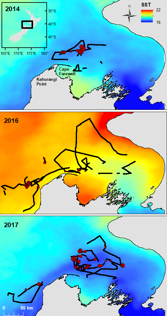
Shifting to an example from another part of the world, the austral summer of 2015-2016 coincided with a strong regional MHW in the Tasman Sea between Australia and New Zealand, which lasted for 251 days and had a maximum intensity of 2.9°C above the climatological average (Oliver et al. 2017). Subsequently, the conditions were linked to a significant shift in zooplankton species composition and abundance in Australia (Evans et al. 2020). Ocean warming, including MHWs, also appears to decrease primary production in the Tasman Sea and large portions of New Zealand’s marine ecosystem (Chiswell & Sutton 2020). In New Zealand’s South Taranaki Bight region, where we study the ecology of blue whales, we observed a shift in blue whale distribution in the MWH conditions of February 2016 relative to more typical ocean conditions in 2014 and 2017 (Fig. 3). The first chapter of my dissertation includes a detailed analysis of the impacts of the 2016 MHW on New Zealand oceanography, krill, and blue whales, documenting how the warm, stratified water column of 2016 led to consequences across multiple trophic levels, from phytoplankton, to zooplankton, to whales.

**Figure 3.** Maps showing monthly sea surface temperature (SST) in the South Taranaki Bight region of New Zealand during our three years of survey effort to document blue whale distribution (February 2014, 2016, and 2017). Vessel tracklines are shown in black, with blue whale sighting locations shown in dark red. Red circles are scaled by the number of blue whales observed at each sighting. The color ramp of SST values is consistent across the three maps, making the dramatically warmer ocean conditions of 2016 evident.

The response of marine mammals is tightly linked to shifts in their environment and prey (Silber et al. 2017). With MHWs and changing ocean conditions, there will likely be “winners” and “losers” among marine predators including large whales. Blue whales are highly selective krill specialists (Nickels et al. 2019), whereas other species of whales, such as humpback whales, have evolved flexible feeding tactics that allow them to switch target prey species when needed (Cade et al. 2020). In California, humpback whales have been shown to switch their primary prey from krill to fish during warm years (Fossette et al. 2017, Santora et al. 2020). By contrast, blue whales shift their distribution in response to changing krill availability during warm years (Fossette et al. 2017), however this strategy comes with increased risk and energetic cost associated with searching for prey in new areas. Furthermore, in instances when a prey resource such as krill becomes increasingly scarce for a multi-year period (Santora et al. 2020), krill specialist predators such as blue whales are at a considerable disadvantage. It is also important to acknowledge that although the humpbacks in California may at first seem to have a winning strategy for adaptation by switching their food source, this tactic may come with unforeseen consequences. Their distribution overlapped substantially with Dungeness crab fishing gear during MHW conditions in the warm blob years, resulting in record numbers of entanglements that may have population-level repercussions (Santora et al. 2020).

While this is certainly not the most light-hearted blog topic, I believe it is an important one. As warming ocean temperatures contribute to the increase in frequency, intensity, and duration of extreme conditions such as MHW events, it is paramount that we understand their impacts and take informed management actions to mitigate consequences, such as lethal entanglements as a result of compressed whale habitat. But perhaps more importantly, even as we do our best to manage consequences, it is critical that we as individuals realize the role we have to play in reducing the root cause of warming oceans, by being conscious consumers and being mindful of the impact our actions have on the climate.

References

Cade DE, Carey N, Domenici P, Potvin J, Goldbogen JA (2020) Predator-informed looming stimulus experiments reveal how large filter feeding whales capture highly maneuverable forage fish. Proc Natl Acad Sci USA.

Chiswell SM, Sutton PJH (2020) Relationships between long-term ocean warming, marine heat waves and primary production in the New Zealand region. New Zeal J Mar Freshw Res.

Evans R, Lea MA, Hindell MA, Swadling KM (2020) Significant shifts in coastal zooplankton populations through the 2015/16 Tasman Sea marine heatwave. Estuar Coast Shelf Sci.

Fossette S, Abrahms B, Hazen EL, Bograd SJ, Zilliacus KM, Calambokidis J, Burrows JA, Goldbogen JA, Harvey JT, Marinovic B, Tershy B, Croll DA (2017) Resource partitioning facilitates coexistence in sympatric cetaceans in the California Current. Ecol Evol.

Hobday AJ, Alexander L V., Perkins SE, Smale DA, Straub SC, Oliver ECJ, Benthuysen JA, Burrows MT, Donat MG, Feng M, Holbrook NJ, Moore PJ, Scannell HA, Sen Gupta A, Wernberg T (2016) A hierarchical approach to defining marine heatwaves. Prog Oceanogr.

Nickels CF, Sala LM, Ohman MD (2019) The euphausiid prey field for blue whales around a steep bathymetric feature in the southern California current system. Limnol Oceanogr.

Oliver ECJ, Benthuysen JA, Bindoff NL, Hobday AJ, Holbrook NJ, Mundy CN, Perkins-Kirkpatrick SE (2017) The unprecedented 2015/16 Tasman Sea marine heatwave. Nat Commun.

Oliver ECJ, Donat MG, Burrows MT, Moore PJ, Smale DA, Alexander L V., Benthuysen JA, Feng M, Sen Gupta A, Hobday AJ, Holbrook NJ, Perkins-Kirkpatrick SE, Scannell HA, Straub SC, Wernberg T (2018) Longer and more frequent marine heatwaves over the past century. Nat Commun.

Santora JA, Mantua NJ, Schroeder ID, Field JC, Hazen EL, Bograd SJ, Sydeman WJ, Wells BK, Calambokidis J, Saez L, Lawson D, Forney KA (2020) Habitat compression and ecosystem shifts as potential links between marine heatwave and record whale entanglements. Nat Commun.

Silber GK, Lettrich MD, Thomas PO, Baker JD, Baumgartner M, Becker EA, Boveng P, Dick DM, Fiechter J, Forcada J, Forney KA, Griffis RB, Hare JA, Hobday AJ, Howell D, Laidre KL, Mantua N, Quakenbush L, Santora JA, Stafford KM, Spencer P, Stock C, Sydeman W, Van Houtan K, Waples RS (2017) Projecting marine mammal distribution in a changing climate. Front Mar Sci.

Marine Mammal Observing: Standardization is key

By: Alexa Kownacki, Ph.D. Student, OSU Department of Fisheries and Wildlife, Geospatial Ecology of Marine Megafauna Lab

For the past two years, I’ve had the opportunity to be the marine mammal observer aboard the NOAA ship Bell M. Shimada for 10 days in May. Both trips covered transects in the Northern California Current Ecosystem during the same time of year, but things looked very different from my chair on the fly bridge. This trip, in particular, highlighted the importance of standardization, seeing as it was the second replicate of the same area. Other scientists and crew members repeatedly asked me the same questions that made me realize just how important it is to have standards in scientific practices and communicating them.

Northern right whale dolphin porpoising out of the water beside the ship while in transit. May 2019. Image source: Alexa Kownacki

The questions:

What do you actually do here and why are you doing it?
Is this year the same as last year in terms of weather, sightings, and transect locations?
Did you expect to see greater or fewer sightings (number and diversity)?
What is this Beaufort Sea State scale that you keep referring to?

All of these are important scientific questions that influence our hypothesis-testing research, survey methods, expected results, and potential conclusions. Although the entire science party aboard the ship conducted marine science, we all had our own specialties and sometimes only knew the basics, if that, about what the other person was doing. It became a perfect opportunity to share our science and standards across similar, but different fields.

Now, to answer those questions:

a) What do you actually do here and b) why are you doing it?

a) As the only marine mammal observer, I stand watch during favorable weather conditions while the ship is in transit, scanning from 0 to 90 degrees off the starboard side (from the front of the ship to a right angle towards the right side when facing forwards). Meanwhile, an application on an iPad called SeaScribe, records the ship’s exact location every 15 seconds, even when no animal is sighted. This process allows for the collection of absence data, that is, data when no animals are present. The SeaScribe program records the survey lines, along with manual inputs that I add, including weather and observer information. When I spot a marine mammal, I immediately mark an exact location on a hand held GPS, use my binoculars to identify the species, and add information to the sighting on the SeaScribe program, such as species, distance to the sighted animal(s), the degree (angle) to the sighting, number of animals in a group, behavior, and direction if traveling.

b) Marine mammal observing serves many different purposes. In this case, observing collects information about what species are where at what time. By piggy-backing on these large-scale, offshore oceanographic NOAA surveys, we have the unique opportunity to survey along standardized transect lines during different times of the year. From replicate survey data, we can start to form an idea of which species use which areas and what oceanographic conditions may impact species distributions. Currently there is not much consistent marine mammal data collected over these offshore areas between Northern California and Washington State, so our work is aiming to fill this knowledge gap.

Alexa observing on the R/V Shimada in May 2019, all bundled up. Image Source: Alexa Kownacki

What is this Beaufort Sea State scale that you keep referring to?

Great question! It took me a while to realize that this standard measuring tool to estimate wind speeds and sea conditions, is not commonly recognized even among other sea-goers. The Beaufort Sea State, or BSS, uses an empirical scale that ranges from 0-12 with 0 being no wind and calm seas, to 12 being hurricane-force winds with 45+ ft seas. It is frequently referenced by scientists in oceanography, marine science, and climate science as a universally-understood metric. The BSS was created in 1805 by Francis Beaufort, a hydrographer in the Royal Navy, to standardize weather conditions across the fleet of vessels. By the mid-1850s, the BSS was standardized to non-naval use for sailing vessels, and in 1916, expanded to include information specific to the seas and not the sails¹. We in the marine mammal observation field constantly collect BSS information while on survey to measure the quality of survey conditions that may impact our observations. BSS data allows us to measure the extent of our survey range, both in the distance that we are likely to sight animals and also the likelihood of sighting anything. Therefore, the BSS scale gives us an important indication of how much absence data we have collected, in addition to presence data.

A description of the Beaufort Sea State Scale. Image source: National Weather Service.

Is this year the same as last year in terms of weather, sightings, and transect locations?

The short answer is no. Observed differences in marine mammal sightings in terms of both species diversity and number of animals between years can be normal. There are many potential explanatory variables, from differences in currents, upwelling strength, El Nino index levels, water temperatures, or, what was obvious in this case: sighting conditions. The weather in May 2019 varied greatly from that in May 2018. Last year, I observed for nearly every day because the Beaufort Sea State (BSS) was frequently less than a four. However, this year, more often than not, the BSS greater than or equal to five. A BSS of 5 equates to approximately 17-21 knots of breeze with 6-foot waves and the water appears to have many “white horses” or pronounced white caps with sea spray. Additionally, mechanical issue with winches delayed and altered our transect locations. Therefore, although multiple transects from May 2018 were also surveyed during May 2019, there were a few lines that do not have data for both cruises.

Did you expect to see greater or fewer sightings (number and diversity)?

Knowing that I had less favorable sighting conditions and less amount of effort observing this year, it is not surprising that I observed fewer marine mammals in total count and in species diversity. Even less surprising is that on the day with the best weather, where the BSS was less than a five, I recorded the most sightings with the highest species count. May 2018 felt a bit like a tropical vacation because we had surprisingly sunny days with mild winds, and during May 2019 we had some rough seas with gale force winds. Additionally, as an observer, I need to remove as much bias as possible. So, yes, I had hoped to see beaked whales or orca like I did in May 2018, but I was still pleasantly surprised when I spotted fin whales feeding in May 2019.

Marine Mammal Species	Number of Sightings
	May 2018	May 2019
Humpback whale	31	6
Northern right whale dolphin	1	2
Pacific white-sided dolphin	3	6
UNID beaked whale	1	0
Cuvier’s beaked whale	1	0
Gray whale	4	1
Minke whale	1	1
Fin whale	4	1
Blue whale	1	0
Transient killer whale	1	0
Dall’s porpoise	2	0
Northern fur seal	1	0
California sea lion	0	1

Pacific white-sided dolphin. Image source: Alexa Kownacki

Standardization is a common theme. Observing between years on standard transects, at set speeds, in different conditions using standardized tools is critical to collecting high quality data that is comparable across different periods. Scientists constantly think about quality control. We look for trends and patterns, similarities and differences, but none of those could be understood without having standard metrics.

The entire science party aboard the R/V Shimada in May 2019, including a marine mammal scientist, phytoplankton scientists, zooplankton scientists, and fisheries scientists, and oceanographers. Image Source: Alexa Kownacki

Literature Cited:

¹Oliver, John E. (2005). Encyclopedia of world climatology. Springer.

Over the Ocean and Under the Bridges: STEM Cruise on the R/V Oceanus

By Alexa Kownacki, Ph.D. Student, OSU Department of Fisheries and Wildlife, Geospatial Ecology of Marine Megafauna Lab

From September 22^nd through 30^th, the GEMM Lab participated in a STEM research cruise aboard the R/V Oceanus, Oregon State University’s (OSU) largest research vessel, which served as a fully-functioning, floating, research laboratory and field station. The STEM cruise focused on integrating science, technology, engineering and mathematics (STEM) into hands-on teaching experiences alongside professionals in the marine sciences. The official science crew consisted of high school teachers and students, community college students, and Oregon State University graduate students and professors. As with a usual research cruise, there was ample set-up, data collection, data entry, experimentation, successes, and failures. And because everyone in the science party actively participated in the research process, everyone also experienced these successes, failures, and moments of inspiration.

The science party enjoying the sunset from the aft deck with the Astoria-Megler bridge in the background. (Image source: Alexa Kownacki)

Dr. Leigh Torres, Dr. Rachael Orben, and I were all primarily stationed on flybridge—one deck above the bridge—fully exposed to the elements, at the highest possible location on the ship for best viewing. We scanned the seas in hopes of spotting a blow, a splash, or any sign of a marine mammal or seabird. Beside us, students and teachers donned binoculars and positioned themselves around the mast, with Leigh and I taking a 90-degree swath from the mast—either to starboard or to port. For those who had not been part of marine mammal observations previously, it was a crash course into the peaks and troughs—of both the waves and of the sightings. We emphasized the importance of absence data: knowledge of what is not “there” is equally as important as what is. Fortunately, Leigh chose a course that proved to have surprisingly excellent environmental conditions and amazing sightings. Therefore, we collected a large amount of presence data: data collected when marine mammals or seabirds are present.

High school student, Chris Quashnick Holloway, records a seabird sighting for observer, Dr. Rachael Orben. (Image source: Alexa Kownacki).

When someone sighted a whale that surfaced regularly, we assessed the conditions: the sea state, the animal’s behavior, the wind conditions, etc. If we deemed them as “good to fly”, our licensed drone pilot and Orange Coast Community College student, Jason, prepared his Phantom 4 drone. While he and Leigh set up drone operations, I and the other science team members maintained a visual on the whale and stayed in constant communication with the bridge via radio. When the drone was ready, and the bridge gave the “all clear”, Jason launched his drone from the aft deck. Then, someone tossed an unassuming, meter-long, wood plank overboard—keeping it attached to the ship with a line. This wood board serves as a calibration tool; the drone flies over it at varying heights as determined by its built-in altimeter. Later, we analyze how many pixels one meter occupied at different heights and can thereby determine the body length of the whale from still images by converting pixel length to a metric unit.

High school student, Alishia Keller, uses binoculars to observe a whale, while PhD student, Alexa Kownacki, radios updates on the whale’s location to the bridge and the aft deck. (Image source: Tracy Crews)

Finally, when the drone is calibrated, I radio the most recent location of our animal. For example, “Blow at 9 o’clock, 250 meters away”. Then, the bridge and I constantly adjust the ship’s speed and location. If the whale “flukes” (dives and exposes the ventral side of its tail), and later resurfaced 500 meters away at our 10 o’clock, I might radio to the bridge to, “turn 60 degrees to port and increase speed to 5 knots”. (See the Hidden Math Lesson below). Jason then positions the drone over the whale, adjusting the camera angle as necessary, and recording high-quality video footage for later analysis. The aerial viewpoint provides major advantages. Whales usually expose about 10 percent of their body above the water’s surface. However, with an aerial vantage point, we can see more of the whale and its surroundings. From here, we can observe behaviors that are otherwise obscured (Torres et al. 2018), and record footage that to help quantify body condition (i.e. lengths and girths). Prior to the batteries running low, Jason returns the drone back to the aft deck, the vessel comes to an idle, and Leigh catches the drone. Throughout these operations, those of us on the flybridge photograph flukes for identification and document any behaviors we observe. Later, we match the whale we sighted to the whale that the drone flew over, and then to prior sightings of this same individual—adding information like body condition or the presence of a calf. I like to think of it as whale detective work. Moreover, it is a team effort; everyone has a critical role in the mission. When it’s all said and done, this noninvasive approach provides life history context to the health and behaviors of the animal.

Drone pilot, Jason Miranda, flying his drone using his handheld ground station on the aft deck. (Photo source: Tracy Crews)

Hidden Math Lesson: The location of 10 o’clock and 60 degrees to port refer to the exact same direction. The bow of the ship is our 12 o’clock with the stern at our 6 o’clock; you always orient yourself in this manner when giving directions. The same goes for a compass measurement in degrees when relating the direction to the boat: the bow is 360/0. An angle measure between two consecutive numbers on a clock is: 360 degrees divided by 12-“hour” markers = 30 degrees. Therefore, 10 o’clock was 0 degrees – (2 “hours”)= 0 degrees- (2*30 degrees)= -60 degrees. A negative degree less than 180 refers to the port side (left).

Our trip was chalked full of science and graced with cooperative weather conditions. There were more highlights than I could list in a single sitting. We towed zooplankton nets under the night sky while eating ice cream bars; we sang together at sunset and watched the atmospheric phenomena: the green flash; we witnessed a humpback lunge-feeding beside the ship’s bow; and we saw a sperm whale traveling across calm seas.

Sperm whale surfacing before a long dive.

On this cruise, our lab focused on the marine mammal observations—which proved excellent during the cruise. In only four days of surveying, we had 43 marine mammal sightings containing 362 individuals representing 9 species (See figure 1). As you can see from figure 2, we traveled over shallow, coastal and deep waters, in both Washington and Oregon before inland to Portland, OR. Because we ventured to areas with different bathymetric and oceanographic conditions, we increased our likelihood of seeing a higher diversity of species than we would if we stayed in a single depth or area.

Humpback whale lunge feeding off the bow.

	Number of sightings	Total number of individuals
Humpback whale	22	40
Pacific white-sided dolphin	3	249
Northern right whale dolphin	1	9
Killer whale	1	3
Dall’s porpoise	5	49
Sperm whale	1	1
Gray whale	1	1
Harbor seal	1	1
California sea lion	8	9
Total	43	362

Figure 1. Summary table of all species sightings during cruise while the science team observed from the flybridge.

Pacific white-sided dolphins swimming towards the vessel.

Figure 2. Map with inset displaying study area and sightings observed by species during the cruise, made in ArcMap. (Image source: Alexa Kownacki).

Even after two days of STEM outreach events in Portland, we were excited to incorporate more science. For the transit from Portland, OR to Newport, OR, the entire science team consisted two people: me and Jason. But even with poor weather conditions, we still used science to answer questions and help us along our journey—only with different goals than on our main leg. With the help of the marine technician, we set up a camera on the bow of the ship, facing aft to watch the vessel maneuver through the famous Portland bridges.

Video 1. Time-lapse footage of the R/V Oceanus maneuvering the Portland Bridges from a GoPro. Compiled by Alexa Kownacki, assisted by Jason Miranda and Kristin Beem.

Prior to the crossing the Columbia River bar and re-entering the Pacific Ocean, the R/V Oceanus maneuvered up the picturesque Columbia River. We used our geospatial skills to locate our fellow science team member and high school student, Chris, who was located on land. We tracked each other using GPS technology in our cell phones, until the ship got close enough to use natural landmarks as reference points, and finally we could use our binoculars to see Chris shining a light from shore. As the ship powered forward and passed under the famous Astoria-Megler bridge that connects Oregon to Washington, Chris drove over it; he directed us “100 degrees to port”. And, thanks to clear directions, bright visual aids, and spatiotemporal analysis, we managed to find our team member waving from shore. This is only one of many examples that show how in a few days at sea, students utilized new skills, such as marine mammal observational techniques, and honed them for additional applications.

On the bow, Alexa and Jason use binoculars to find Chris–over 4 miles–on the Washington side of the Columbia River. (Image source: Kristin Beem)

Great science is the result of teamwork, passion, and ingenuity. Working alongside students, teachers, and other, more-experienced scientists, provided everyone with opportunities to learn from each other. We created great science because we asked questions, we passed on our knowledge to the next person, and we did so with enthusiasm.

High school students, Jason and Chris, alongside Dr. Leigh Torres, all try to get a glimpse at the zooplankton under Dr. Kim Bernard’s microscope. (Image source: Tracy Crews).

Check out other blog posts written by the science team about the trip here.

Finding the right fit: a journey into cetacean distribution models

Solène Derville, Entropie Lab, French National Institute for Sustainable Development (IRD – UMR Entropie), Nouméa, New Caledonia

Ph.D. student under the co-supervision of Dr. Leigh Torres

Species Distribution Models (SDM), also referred to as ecological niche models, may be defined as “a model that relates species distribution data (occurrence or abundance at known locations) with information on the environmental and/or spatial characteristics of those locations” (Elith & Leathwick, 2009)⁠. In the last couple decades, SDMs have become an indispensable part of the ecologists’ and conservationists’ toolbox. What scientist has not dreamed of being able to summarize a species’ environmental requirements and predict where and when it will occur, all in one tiny statistical model? It sounds like magic… but the short acronym “SDM” is the pretty front window of an intricate and gigantic research field that may extend way beyond the skills of a typical ecologist (even so for a graduate student like myself).

As part of my PhD thesis about the spatial ecology of humpback whales in New Caledonia, South Pacific, I was planning on producing a model to predict their distribution in the region and help spatial planning within the Natural Park of the Coral Sea. An innocent and seemingly perfectly feasible plan for a second year PhD student. To conduct this task, I had at my disposal more than 1,000 sightings recorded during dedicated surveys at sea conducted over 14 years. These numbers seem quite sufficient, considering the rarity of cetaceans and the technical challenges of studying them at sea. And there was more! The NGO Opération Cétacés also recorded over 600 sightings reported by the general public in the same time period and deployed more than 40 satellite tracking tags to follow individual whale movements. In a field where it is so hard to acquire data, it felt like I had to use it all, though I was not sure how to combine all these types of data, with their respective biases, scales and assumptions.

One important thing about SDM to remember: it is like a cracker section in a US grocery shop, there is sooooo much choice! As I reviewed the possibilities and tested various modeling approaches on my data I realized that this study might be a good opportunity to contribute to the SDM field, by conducting a comparison of various algorithms using cetacean occurrence data from multiple sources. The results of this work was just published in Diversity and Distributions:

Derville S, Torres LG, Iovan C, Garrigue C. (2018) Finding the right fit: Comparative cetacean distribution models using multiple data sources and statistical approaches. Divers Distrib. 2018;00:1–17. https://doi. org/10.1111/ddi.12782

There are simply too many! Anonymous grocery shops, Corvallis, OR
Credit: Dawn Barlow

If you are a new-comer to the SDM world, and specifically its application to the marine environment, I hope you find this interesting. If you are a seasoned SDM user, I would be very grateful to read your thoughts in the comment section! Feel free to disagree!

So what is the take-home message from this work?

There is no such thing as a “best model”; it all depends on what you want your model to be good at (the descriptive vs predictive dichotomy), and what criteria you use to define the quality of your models.

The predictive vs descriptive goal of the model: This is a tricky choice to make, yet it should be clearly identified upfront. Most times, I feel like we want our models to be decently good at both tasks… It is a risky approach to blindly follow the predictions of a complex model without questioning the meaning of the ecological relationships it fitted. On the other hand, conservation applications of models often require the production of predicted maps of species’ probability of presence or habitat suitability.

The criteria for model selection: How could we imagine that the complexity of animal behavior could be summarized in a single metric, such as the famous Akaike Information criterion (AIC) or the Area under the ROC Curve (AUC)? My study, and that of others (e.g. Elith & Graham H., 2009),⁠ emphasize the importance of looking at multiple aspects of model outputs: raw performance through various evaluation metrics (e.g. see AUCdiff; (Warren & Seifert, 2010)⁠, contribution of the variables to the model, shape of the fitted relationships through Partial Dependence Plots (PDP, Friedman, 2001),⁠ and maps of predicted habitat suitability and associated error. Spread all these lines of evidence in front of you, summarize all the metrics, add a touch of critical ecological thinking to decide on the best approach for your modeling question, and Abracadabra! You end up a bit lost in a pile of folders… But at least you assessed the quality of your work from every angle!

Cetacean SDMs often serve a conservation goal. Hence, their capacity to predict to areas / times that were not recorded in the data (which is often scarce) is paramount. This extrapolation performance may be restricted when the model relationships are overfitted, which is when you made your model fit the data so closely that you are unknowingly modeling noise rather than a real trend. Using cross-validation is a good method to prevent overfitting from happening (for a thorough review: Roberts et al., 2017)⁠. Also, my study underlines that certain algorithms inherently have a tendency to overfit. We found that Generalized Additive Models and MAXENT provided a valuable complexity trade-off to promote the best predictive performance, while minimizing overfitting. In the case of GAMs, I would like to point out the excellent documentation that exist on their use (Wood, 2017)⁠, and specifically their application to cetacean spatial ecology (Mannocci, Roberts, Miller, & Halpin, 2017; Miller, Burt, Rexstad, & Thomas, 2013; Redfern et al., 2017).⁠

Citizen science is a promising tool to describe cetacean habitat. Indeed, we found that models of habitat suitability based on citizen science largely converged with those based on our research surveys. The main issue encountered when modeling this type of data is the absence of “effort”. Basically, we know where people observed whales, but we do not know where they haven’t… or at least not with the accuracy obtained from research survey data. However, with some information about our citizen scientists and a little deduction, there is actually a lot you can infer about opportunistic data. For instance, in New Caledonia most of the sightings were reported by professional whale-watching operators or by the general public during fishing/diving/boating day trips. Hence, citizen scientists rarely stray far from harbors and spend most of their time in the sheltered waters of the New Caledonian lagoon. This reasoning provides the sort of information that we integrated in our modeling approach to account for spatial sampling bias of citizen science data and improve the model’s predictive performance.

Many more technical aspects of SDM are brushed over in this paper (for detailed and annotated R codes of the modeling approaches, see supplementary information of our paper). There are a few that are not central to the paper, but that I think are worth sharing:

Collinearity of predictors: Have you ever found that the significance of your predictors completely changed every time you removed a variable? I have progressively come to discover how unstable a model can be because of predictor collinearity (and the uneasy feeling that comes with it …). My new motto is to ALWAYS check cross-correlation between my predictors, and do it THOROUGHLY. A few aspects that may make a big difference in the estimation of collinearity patterns are to: (1) calculate Pearson vs Spearman coefficients, (2) check correlations between the values recorded at the presence points vs over the whole study area, and (3) assess the correlations between raw environmental variables vs between transformed variables (log-transformed, etc). Though selecting variables with Pearson coefficients < 0.7 is usually a good rule (Dormann et al., 2013), I would worry of anything above 0.5, or at least keep it in mind during model interpretation.

Cross-validation: If removing 10% of my dataset greatly impacts the model results, I feel like cross-validation is critical. The concept is based on a simple assumption, if I had sampled a given population/phenomenon/system slightly differently, would I have come to the same conclusion? Cross-validation comes in many different methods, but the basic concept is to run the same model several times (number of times may depend on the size of your data set, hierarchical structure of your data, computation power of your computer, etc.) over different chunks of your data. Model performance metrics (e.g., AUC) and outputs (e.g., partial dependence plots) are than summarized on the many runs, using mean/median and standard deviation/quantiles. It is up to you how to pick these chunks, but before doing this at random I highly recommend reading Roberts et al. (2017).

The evil of the R²: I am probably not the first student to feel like what I have learned in my statistical classes at school is in practice, at best, not very useful, and at worst, dangerously misleading. Of course, I do understand that we must start somewhere, and that learning the basics of inferential statistics is a necessary step to, one day, be able to answer your one research questions. Yet, I feel like I have been carrying the “weight of the R²” for far too long before actually realizing that this metric of model performance (R² among others) is simply not enough to trust my results. You might think that your model is robust because among the 1000 alternative models you tested, it is the one with the “best” performance (deviance explained, AIC, you name it), but the model with the best R² will not always be the most ecologically meaningful one, or the most practical for spatial management perspectives. Overfitting is like a sword of Damocles hanging over you every time you create a statistical model All together, I sometimes trust my supervisor’s expertise and my own judgment more than an R².

A few good websites/presentations that have helped me through my SDM journey:

General website about spatial analysis (including SDM): http://rspatial.org/index.html

Cool presentation by Adam Smith about SDM:

http://www.earthskysea.org/!ecology/sdmShortCourseKState2012/sdmShortCourse_kState.pdf

Handling spatial data in R: http://www.maths.lancs.ac.uk/~rowlings/Teaching/UseR2012/introductionTalk.html

“The magical world of mgcv”, a great presentation by Noam Ross: https://www.youtube.com/watch?v=q4_t8jXcQgc

Literature cited

Dormann, C. F., Elith, J., Bacher, S., Buchmann, C., Carl, G., Carré, G., … Lautenbach, S. (2013). Collinearity: A review of methods to deal with it and a simulation study evaluating their performance. Ecography, 36(1), 027–046. https://doi.org/10.1111/j.1600-0587.2012.07348.x

Elith, J., & Graham H., C. (2009). Do they? How do they? WHY do they differ? On ﬁnding reasons for differing performances of species distribution models . Ecography, 32(Table 1), 66–77. https://doi.org/10.1111/j.1600-0587.2008.05505.x

Elith, J., & Leathwick, J. R. (2009). Species Distribution Models: Ecological Explanation and Prediction Across Space and Time. Annual Review of Ecology, Evolution, and Systematics, 40(1), 677–697. https://doi.org/10.1146/annurev.ecolsys.110308.120159

Friedman, J. H. (2001). Greedy Function Approximation: A gradient boosting machine. The Annals of Statistics, 29(5), 1189–1232. Retrieved from http://www.jstor.org/stable/2699986

Mannocci, L., Roberts, J. J., Miller, D. L., & Halpin, P. N. (2017). Extrapolating cetacean densities to quantitatively assess human impacts on populations in the high seas. Conservation Biology, 31(3), 601–614. https://doi.org/10.1111/cobi.12856.This

Miller, D. L., Burt, M. L., Rexstad, E. A., & Thomas, L. (2013). Spatial models for distance sampling data: Recent developments and future directions. Methods in Ecology and Evolution, 4(11), 1001–1010. https://doi.org/10.1111/2041-210X.12105

Redfern, J. V., Moore, T. J., Fiedler, P. C., de Vos, A., Brownell, R. L., Forney, K. A., … Ballance, L. T. (2017). Predicting cetacean distributions in data-poor marine ecosystems. Diversity and Distributions, 23(4), 394–408. https://doi.org/10.1111/ddi.12537

Roberts, D. R., Bahn, V., Ciuti, S., Boyce, M. S., Elith, J., Guillera-Arroita, G., … Dormann, C. F. (2017). Cross-validation strategies for data with temporal, spatial, hierarchical or phylogenetic structure. Ecography, 0, 1–17. https://doi.org/10.1111/ecog.02881

Warren, D. L., & Seifert, S. N. (2010). Ecological niche modeling in Maxent: the importance of model complexity and the performance of model selection criteria. Ecological Applications, 21(2), 335–342. https://doi.org/10.1890/10-1171.1

Wood, S. N. (2017). Generalized additive models: an introduction with R (second edi). CRC press.

The Recipe for a “Perfect” Marine Mammal and Seabird Cruise

By Alexa Kownacki, Ph.D. Student, OSU Department of Fisheries and Wildlife, Geospatial Ecology of Marine Megafauna Lab

Science—and fieldwork in particular—is known for its failures. There are websites, blogs, and Twitter pages dedicated to them. This is why, when things go according to plan, I rejoice. When they go even better than expected, I practically tear up from amazement. There is no perfect recipe for a great marine mammal and seabird research cruise, but I would suggest that one would look like this:

A Great Marine Mammal and Seabird Research Cruise Recipe:

A heavy pour of fantastic weather
- Light on the wind and seas
- Light on the glare
Equal parts amazing crew and good communication
A splash of positivity
A dash of luck
A pinch of delicious food
Heaps of marine mammal and seabird sightings
Heat to approximately 55-80 degrees F and transit for 10 days along transects at 10-12 knots

The end of another beautiful day at sea on the R/V Shimada. Image source: Alexa K.

The Northern California Current Ecosystem (NCCE) is a highly productive area that is home to a wide variety of cetacean species. Many cetaceans are indicator species of ecosystem health as they consume large quantities of prey from different levels in trophic webs and inhabit diverse areas—from deep-diving beaked whales to gray whales traveling thousands of miles along the eastern north Pacific Ocean. Because cetacean surveys are a predominant survey method in large bodies of water, they can be extremely costly. One alternative to dedicated cetacean surveys is using other research vessels as research platforms and effort becomes transect-based and opportunistic—with less flexibility to deviate from predetermined transects. This decreases expenses, creates collaborative research opportunities, and reduces interference in animal behavior as they are never pursued. Observing animals from large, motorized, research vessels (>100ft) at a steady, significant speed (>10kts/hour), provides a baseline for future, joint research efforts. The NCCE is regularly surveyed by government agencies and institutions on transects that have been repeated nearly every season for decades. This historical data provides critical context for environmental and oceanographic dynamics that impact large ecosystems with commercial and recreational implications.

My research cruise took place aboard the 208.5-foot R/V Bell M. Shimada in the first two weeks of May. The cruise was designated for monitoring the NCCE with the additional position of a marine mammal observer. The established guidelines did not allow for deviation from the predetermined transects. Therefore, mammals were surveyed along preset transects. The ship left port in San Francisco, CA and traveled as far north as Cape Meares, OR. The transects ranged from one nautical mile from shore and two hundred miles offshore. Observations occurred during “on effort” which was defined as when the ship was in transit and moving at a speed above 8 knots per hour dependent upon sea state and visibility. All observations took place on the flybridge during conducive weather conditions and in the bridge (one deck below the flybridge) when excessive precipitation was present. The starboard forward quarter: zero to ninety degrees was surveyed—based on the ship’s direction (with the bow at zero degrees). Both naked eye and 7×50 binoculars were used with at least 30 percent of time binoculars in use. To decrease observer fatigue, which could result in fewer detected sightings, the observer (me) rotated on a 40 minutes “on effort”, 20 minutes “off effort” cycle during long transits (>90 minutes).

Alexa on-effort using binoculars to estimate the distance and bearing of a marine mammal sighted off the starboard bow. Image source: Alexa K.

Data was collected using modifications to the SEEbird Wincruz computer program on a ruggedized laptop and a GPS unit was attached. At the beginning of each day and upon changes in conditions, the ship’s heading, weather conditions, visibility, cloud cover, swell height, swell direction, and Beaufort sea state (BSS) were recorded. Once the BSS or visibility was worse than a “5” (1 is “perfect” and 5 is “very poor”) observations ceased until there was improvement in weather. When a marine mammal was sighted the latitude and longitude were recorded with the exact time stamp. Then, I noted how the animal was sighted—either with binoculars or naked eye—and what action was originally noticed—blow, splash, bird, etc. The bearing and distance were noted using binoculars. The animal was given three generalized behavior categories: traveling, feeding, or milling. A sighting was defined as any marine mammal or group of animals. Therefore, a single sighting would have the species and the best, high, and low estimates for group size.

By my definitions, I had the research cruise of my dreams. There were moments when I imagined people joining this trip as a vacation. I *almost* felt guilty. Then, I remember that after watching water for almost 14 hours (thanks to the amazing weather conditions), I worked on data and reports and class work until midnight. That’s the part that no one talks about: the data. Fieldwork is about collecting data. It’s both what I live for and what makes me nervous. The amount of time, effort, and money that is poured into fieldwork is enormous. The acquisition of the data is not as simple as it seems. When I briefly described my position on this research cruise to friends, they interpret it to be something akin to whale-watching. To some extent, this is true. But largely, it’s grueling hours that leave you fatigued. The differences between fieldwork and what I’ll refer to as “everything else” AKA data analysis, proposal writing, manuscript writing, literature reviewing, lab work, and classwork, are the unbroken smile, the vaguely tanned skin, the hours of laughter, the sea spray, and the magical moments that reassure me that I’ve chosen the correct career path.

Alexa photographing a gray whale at sunset near Newport, OR. Image source: Alexa K.

This cruise was the second leg of the Northern California Current Ecosystem (NCCE) survey, I was the sole Marine Mammal and Seabird Observer—a coveted position. Every morning, I would wake up at 0530hrs, grab some breakfast, and climb to the highest deck: the fly-bridge. Akin to being on the top of the world, the fly-bridge has the best views for the widest span. From 0600hrs to 2000hrs I sat, stood, or danced in a one-meter by one-meter corner of the fly-bridge and surveyed. This visual is why people think I’m whale watching. In reality, I am constantly busy. Nonetheless, I had weather and seas that scientists dream about—and for 10 days! To contrast my luck, you can read Florence’s blog about her cruise. On these same transects, in February, Florence experienced 20-foot seas with heavy rain with very few marine mammal sightings—and of those, the only cetaceans she observed were gray whales close to shore. That starkly contrasts my 10 cetacean species with upwards of 45 sightings and my 20-minute hammock power naps on the fly-bridge under the warm sun.

Pacific white-sided dolphins traveling nearby. Image source: Alexa K.

Marine mammal sightings from this cruise included 10 cetacean species: Pacific white-sided dolphin, Dall’s porpoise, unidentified beaked whale, Cuvier’s beaked whale, gray whale, Minke whale, fin whale, Northern right whale dolphin, blue whale, humpback whale, and transient killer whale and one pinniped species: northern fur seal. What better way to illustrate these sightings than with a map? We are a geospatial lab after all.

Cetacean Sightings on the NCCE Cruise in May 2018. Image source: Alexa K.

This map is the result of data collection. However, it does not capture everything that was observed: sea state, weather, ocean conditions, bathymetry, nutrient levels, etc. There are many variables that can be added to maps–like this one (thanks to my GIS classes I can start adding layers!)–that can provide a better understanding of the ecosystem, predator-prey dynamics, animal behavior, and population health.

The catch from a bottom trawl at a station with some fish and a lot of pyrosomes (pink tube-like creatures). Image source: Alexa K.

Being a Ph.D. student can be physically and mentally demanding. So, when I was offered the opportunity to hone my data collection skills, I leapt for it. I’m happiest in the field: the wind in my face, the sunshine on my back, surrounded by cetaceans, and filled with the knowledge that I’m following my passion—and that this data is contributing to the greater scientific community.

Humpback whale photographed traveling southbound. Image source: Alexa K.

Wildlife of the Western Antarctic Peninsula

Erin Pickett, MS Student, Fisheries and Wildlife Department, OSU

This time last week, I was on a research vessel crossing the Drake Passage. The Drake extends from the tip of the Western Antarctic Peninsula to South America’s Cape Horn, and was part of the route I was taking home from Antarctica. Over the past three months I have been working on a long-term ecological research (LTER) project based out of Palmer Station, a U.S. based research facility located on Anvers Island.

Image: http://www.tetonat.com/2009/11/06/bon-voyage-off-to-antarctica-with-iceaxe-expeditions/

While in Antarctica, I was working on the cetacean component of the Palmer LTER project, which I’ve described in previous blog posts. In lieu of writing more about what it is like to work and live on the Antarctic Peninsula, I thought I’d share some photos with you. Working on the water everyday while searching for whales provided me with many opportunities to photograph the local wildlife. I hope you’ll enjoy a few of my favorite shots.

Chinstrap penguin (Pygoscelis antarcticus)

Southern elephant seal (Mirounga leonina)

Adelie penguin (Pygoscelis adeliae) colony on Avian Island

Wilson’s storm petrel (Oceanites oceanicus)

Southern fur seal (Arctocephalus gazella)

Blue-eyed shag (Phalacrocorax (atriceps) bransfieldensis)

An update from the Antarctic Peninsula

By: Erin Pickett

Yesterday someone said to me, “I don’t know if it was sunrise or sunset, but it was beautiful”. So it goes on the R/V Lawrence M. Gould (LMG), the surrounding scenery is incredible but the work schedule on this research ship makes it difficult to remember what time of day it is.

Here on the Antarctic Peninsula, the sun never really sets and our daily schedules are dependent on things like the diel vertical migration of krill, the current wind speed and the amount of sea ice in between us and our study species, the humpback whale. For these reasons, we sometimes find ourselves starting our workday at odd hours, like 11:45 pm (or 4:00 am). As a reminder, I am currently working on research vessel on a project called the Palmer long term ecological research (LTER) project. You can read my first blog post about that here. We are about one week into our journey and so far, so good!

Our journey began in Punta Arenas, Chile, where we spent two days loading our research supplies onto the LMG and getting outfitted with cold weather gear. From Punta Arenas we headed south through the straights of Magellan and then across the Drake Passage. Along the way we spotted a variety of cetaceans including minke, fin, sei and humpback whales, and Commerson’s and Peale’s dolphins. I spent as much of our time in transit as I could looking for seabirds, the most numerous being white-chinned and cape petrels, southern giant petrels, and black-browed albatrosses. Spotting either a royal or a wandering albatross was always exciting. An eleven foot wingspan allows these albatross to glide effortlessly above the water and this makes for a beautiful sight!

We have spent the last four days transiting between various sampling stations around Palmer deep, which is an underwater canyon just south of our home base at Palmer station. When conditions allowed, we loaded up our tagging and biopsy gear into a small boat and went to look for humpback whales. We’ve been incredibly successful with the limited amount of time we’ve had on the water and this morning we finished deploying our sixth tag.

We brought a few different types of satellite tags with us to deploy on humpback whales. One type is an implantable satellite tag that transmits location data over a long period of time. These data allow us to gain a better understanding of the large-scale movement and distribution patterns of these animals. The other tag we deploy is a suction cup tag, so called because four small suction cups attach the tag to the whale. These suction cup tags are multi-sensor tags that measure location as well as fine scale underwater movement (e.g. pitch, roll, and heading). They are also equipped with forward and backward facing cameras and most importantly, radio transmitters! This allows us to recover the tags once they fall off the animal and float to the surface (after about 24 hours). The data we get from these tags will allow us to quantify fine-scale foraging behavior in terms of underwater maneuverability, prey type and the frequency, depth and time of day that feeding occurs.

When we deployed each of these tags we also obtained a biopsy sample and fluke photos. Fluke photos and biopsy samples allow us to distinguish between individual animals, and the biopsy samples will also be used to study the demographics of this population through genetic analysis.

Now that we’ve deployed all of our satellite tags and have recovered the suction cup tag just in the nick of time (!), we are starting our first major transect line toward the continental shelf. We will be continuing south along these grid lines for the next week.

My lab mate Logan Pallin and I will be continuing to write about our trip over the next couple of months on another blog we created especially for this project. You can find it here: blogs.oregonstate.edu/LTERcetaceans

I’ll leave you with a few of my favorite photos of the trip so far!