Geospatial Ecology of Marine Megafauna Laboratory

Cooperative Fishing: Symbiotic Relationships between People and Dolphins

By: Alexa Kownacki, Ph.D. Student, OSU Department of Fisheries and Wildlife, Geospatial Ecology of Marine Megafauna Lab

Human-wildlife interactions have occurred since people first inhabited the Earth. However, today, when describing human-wildlife interactions specifically in relation to dolphins, frequently we hear about ‘conflicts’. Interactions between fisheries and dolphins that lead to bycatch or depredation (stealing bait/catching from gear) are particularly common. But, symbiotic relationships with dolphin species and certain human groups can also be mutualistic, with both groups benefitting. These symbiotic relationships have been around for hundreds, if not thousands of years.

A depiction of Aboriginal Australians using nets to catch fish in a small inlet with the assistance of coastal dolphins. (Image source: Our Pacific Ocean)

In eastern Australia, cooperative fishing interactions occur between Aboriginal Australians and dolphins—both bottlenose dolphins and orcas. In Burleigh Heads National Park, Queensland, AUS, the dolphins are thought to help the local indigenous Kombemerri (saltwater) people hunt for fish. Indigenous stories recall men wading into the water with their spears and nets. Then, many of the men would hit the surface waters to make noises with the splashes. Underwater, this sound was amplified and then the dolphins would begin chasing the fish toward the men and their nets (Neil 2002). Aboriginal Australians, especially those in eastern Australia have an emotional and spiritual connection to both dolphins and orcas. There are widespread accounts of cooperation between indigenous people and small cetaceans on the eastern Australian coastline, which create both context and precedent for the economic and emotional objectives to contemporary human-dolphin interactions such as dolphin provisioning (Neil 2002).

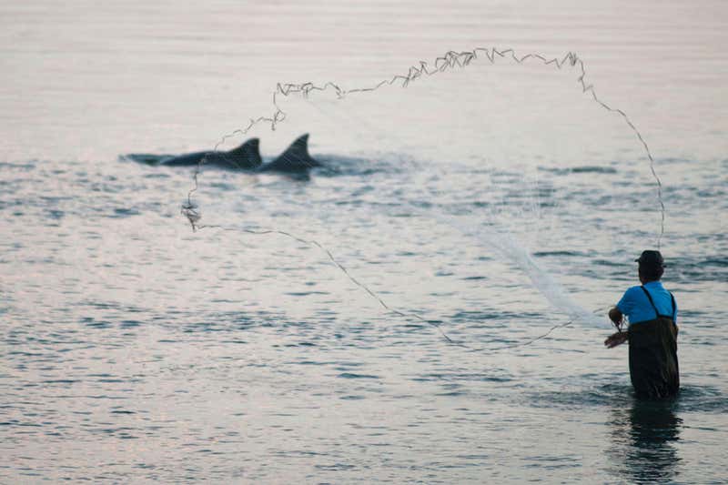
Dolphins and fishermen work together in Laguna, Brazil, to catch mullet. (Image Source: Fábio Daura-Jorge)

In the coasts off of Laguna, Brazil, bottlenose dolphins and local fishermen cooperatively fish while tourists gather to watch. Previously, PhD candidate Leila Lemos wrote about these interactions in a blog post. Like many groups of socializing dolphins, these dolphins have a unique whistle to recognize each other. The waters surrounding Laguna, Brazil are murky, turbid and dark green to the point where the fisherman cannot see any of the fish in the water. As the fishermen wade into the murky waters, bottlenose dolphins chase shoals of mullet toward the shore. Then the dolphins tail slap or abruptly dive, “signaling” the fishermen to cast their nets. Research has shown that when the fishermen “work with” the dolphins, both the dolphins and the people catch more, larger fish (Roman 2013). One fisherman claims it is not worth fishing unless the dolphins are around (Roman 2013). Here, the fishermen know the dolphins based on their markings. They know which dolphins participate in the different parts of hunting as well—which dolphin initiates the tail slap, which dolphin usually circles the fish, and which drive the fish towards the coastline. After the dolphins round up and chase the fish for the fishermen and themselves, there is no “reward” from the fishermen for the dolphins—no fish tossed their way. Scientists also found there is a difference in whistle structure between cooperative and non-cooperative dolphin groups (Preston 2017).

A fisherman in Brazil throws a net after dolphins chase mullet into the shore. (Image Source: Leo Francini:Alamy Stock Photo)

Along most coastlines worldwide, humans and dolphins are competitors. Dolphins are seen as thieves who steal fish out of nets, or get caught in their gear and ruin fishing opportunities. Thus, dolphins are often unwelcome near fishing communities. Such negative interactions sometimes lead to human-caused fatalities of dolphin from gunshots or stabbings, thought to be from angry fishermen. Yet, in this same world, fishermen thank the dolphins for bringing their catch to them. Clearly, both humans and dolphins share high intelligence levels and skills in fishing. If it is a matter of two minds are better than one, then I think indigenous communities figured this equation out first: working with the dolphins, and not against, can better feed their people.

Citations:

Neil, David. (2002). Cooperative fishing interactions between Aboriginal Australians and dolphins in eastern Australia. Anthrozoos: A Multidisciplinary Journal of The Interactions of People & Animals. 15. 10.2752/089279302786992694.

Preston, Elizabeth. “Dolphins That Work with Humans to Catch Fish Have Unique Accent.” New Scientist, 2 Oct. 2017, www.newscientist.com/article/2149139-dolphins-that-work-with-humans-to-catch-fish-have-unique-accent/.

Roman, Joe. “Fishing with Dolphins: An astonishing cooperative venture in which every species wins but the fish.” Slate Magazine, 31 Jan. 2013, slate.com/technology/2013/01/fishing-with-dolphins-symbiosis-between-humans-and-marine-mammals-to-catch-more-fish.html.

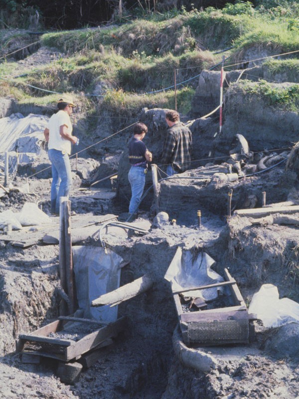
Makah Gray Whale Hunt Waiver – a long-time coming, but still premature?

By Lisa Hildebrand, MSc student, OSU Department of Fisheries & Wildlife, Marine Mammal Institute, Geospatial Ecology of Marine Megafauna Lab

Archaeological site of Ozette Village. Source: Makah Museum.

The Makah, an indigenous people of the Pacific Northwest Coast living in Washington State, have a long history with whaling. Deposits from a mudslide in the village of Ozette suggest that whaling may date back 2,000 years as archaeologists uncovered humpback and gray whale bones and barbs from harpoons (Kirk 1986). However, the history of Makah whaling is also quite recent. On January 29 of this year, the National Marine Fisheries Service (NMFS; informally known as NOAA Fisheries) announced a 45-day public comment period regarding a NMFS proposed waiver on the Marine Mammal Protection Act’s (MMPA) moratorium on the take of marine mammals to allow the Makah to take a limited number of eastern North Pacific gray whales (ENP). To understand how the process reached this point, we first must go back to 1855.

1855 marks the year in which the U.S. government and the Makah entered into the Treaty of Neah Bay (in Washington state). The Makah ceded thousands of acres of land to the U.S. government, and in return reserved their right to whale. Following the treaty, the Makah hunt of gray whales continued until the 1920s. At this point, commercial hunting had greatly reduced the ENP population, so much so that the Makah voluntarily ceased their whaling. The next seven decades brought about the formation of the International Whaling Commission (IWC), the enactment of the Whaling Convention Act, the listing of gray whales as endangered under the U.S. Endangered Species Act, and the enactment of the MMPA. For gray whales, these national and international measures were hugely successful, leading to the removal of the ENP from the Federal List of Endangered Wildlife in 1994 when it was determined that the population had recovered to near its estimated original population size.

One year later on May 5, 1995 (just one month after I was born!), the Makah asked the U.S. Department of Commerce to represent its interest to obtain a quota for gray whales from the IWC in order to resume their treaty right for ceremonial and subsistence harvest of the ENP. The U.S. government pursued this request at the next IWC meeting, and subsequently NMFS issued a final Environmental Assessment that found no significant impact to the ENP population if the hunt recommenced. The IWC set a catch limit and NMFS granted the Makah a quota in 1998. In 1999 the Makah hunted, struck and landed an ENP gray whale.

*“Makahs cutting up whale, Neah Bay, ca. 1930. Photo by Asahel Curtis, Courtesy UW Special Collections (CUR767)”*. Source and caption: History Link.

I will not go into detail about what happened between 1999 and now because frankly, a lot happened, particularly a lot of legal events including summary judgements, appeals, and a lot of other legal jargon that I do not quite understand. If you want to know the specifics of what happened in those two decades, I suggest you look at NMFS’ chronology of the Makah Tribal Whale Hunt. In short, cases brought against NMFS argued that they did not take a “hard [enough] look” at the National Environmental Policy Act when deciding that the Makah could resume the hunt. Consequently, the hunt was put on hold. Yet, in 2005 NMFS received a waiver request from the Makah on the MMPA’s take moratorium and NMFS published a notice of intent to review this request. A lot more happened between that event and now, including on January 29 of this year when NMFS announced the availability of transcripts from the Administrative Law Judge’s (ALJ) hearing (which happened from November 14-21, 2019) on the proposed regulations and waiver to allow the Makah to resume hunting the ENP. We are currently in the middle of the aforementioned 45-day public comment period on the formal rulemaking record.

It has been 15 years since the Makah requested the waiver and while the decision has not yet been reached, we are likely nearing the end of this long process. This blog has turned into somewhat of a history lesson (not really my intention) but I feel it is important to understand the lengthy and complex history associated with the decision that is probably going to happen sometime this year. My actual intent for this blog is to ruminate on a few questions, some of which remain unanswered in my opinion, that are large and broad, and important to consider. Some of these questions point out gaps in our ecological knowledge regarding gray whales that I believe should be addressed for a truly informed decision to be made on NMFS’ proposed waiver now or anytime in the near future.

1. Should the Pacific Coast Feeding Group (PCFG) of gray whales be recognized as its own stock?

Currently, the PCFG are considered a part of the ENP stock. This decision was published following a workshop held by a NMFS task force (Weller et al. 2013). The report concluded that based on photo-identification, genetics, tagging, and other data, there was a substantial level of uncertainty in the strength of the evidence to support the independence of the PCFG from the ENP. Nevertheless, mitochondrial genetic data have indicated a differentiation between the PCFG and the ENP, and the exchange rate between the two groups may be small enough for the two to be considered demographically independent (Frasier et al. 2011). Based on all currently available data, it seems that matrilineal fidelity plays a role in creating population structure within and between the PCFG and the ENP, however there has not been any evidence to suggest that whales from one feeding area (i.e. the PCFG range) are reproductively isolated from whales that utilize other feeding areas (i.e. the Arctic ENP feeding grounds) (Lang et al. 2011). Several PCFG researchers do argue that there needs to be recognition of the PCFG as an independent stock. It is clear that more research, especially efforts to link genetic and photo-identification data within and between groups, is required.

ENP gray whales foraging off the coast of Alaska on their main foraging grounds in the Bering Sea. Photo taken by ASAMM/AFSC. Funded by BOEM IAA No. M11PG00033. Source: NMFS.

2. Is emigration/immigration driving PCFG population growth, or is it births/deaths?

It is unclear whether the current PCFG population growth is a consequence of births and deaths that occur within the group (internal dynamics) or whether it is due to immigration and emigration (external dynamics). Likely, it is a combination of the two, however which of the two has more of an effect or is more prevalent? This question is important to answer because if population growth is driven more by external dynamics, then potential losses to the PCFG population due to the Makah hunt may not be as detrimental to the group as a whole. However, if internal dynamics play a bigger role, then the loss of just a few females could have long-term ramifications for the PCFG (Schubert 2019). NMFS has taken precautions to try and avoid such effects. In their proposed waiver, of the cumulative limit of 16 strikes of PCFG whales over the 10-year waiver period, no more than 8 of the strikes may be PCFG females (Yates 2019a). While a great step, it still begs the question how the loss of 8 females, admittedly over a rather long period of time, may affect population dynamics since we do not know what ultimately drives recruitment. Especially when taken together with potential non-lethal effects on whales (further discussed in question 5 below).

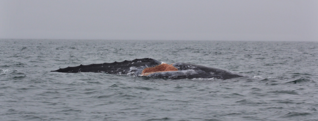
“Scarlet” is a PCFG female who has had multiple calves in the decades that researchers have seen her in the PCFG range. Image captured under NOAA/NMFS permit #21678. Source: L Hildebrand.

3. How important are individual patterns within the PCFG, and how might the loss of these individuals affect the population?

The hunt will be restricted to the Makah Usual & Accustomed fishing area (U&A), which is off the Washington coast. It has been shown that site fidelity among PCFG individuals is strong. In fact, based on the 143 PCFG gray whales observed in nine or more years from 1996 to 2015, 94.4% were seen in at least one of nine different PCFG regions during six or more of the years they were seen (Calambokidis et al. 2017). While high site-fidelity seems to be common for some PCFG individuals in certain regions, interestingly, an analysis of sighting histories of all individuals that utilized the Makah U&A from 1985-2011 revealed that most PCFG whales do not have strong site fidelity to the Makah U&A (Scordino et al. 2017). Only about 20% of the whales were observed in six or more years of the total 26 years of data analyzed. Since high individual site fidelity does not appear to be strong in this area, perhaps a loss of genetic diversity, cultural knowledge, and behavioral individualism is not of great concern.

“Buttons” seems to have a preference for the southern Oregon coast as in the last 5 years the GEMM Lab has conducted research, he has only been sighted in 1 year in Newport but in all 5 years in Port Orford. However, perhaps such preferences are not common among all PCFG whales. Source: F. Sullivan.

4. How has the current UME affected the situation?

The ENP has experienced two Unusual Mortality Events (UMEs) in the past 20 years; one from 1999-2000 and the second began in May 2019. Many questions arise when thinking about the Makah hunt in light of the UME.

What impacts will the current UME have on ENP and PCFG birth rates in subsequent years?
Could the UME lead to shifts in feeding behavior of ENP whales and result in greater use of PCFG range by more individuals?
What caused the UME? Shifting prey availability and a changing climate? Or has the ENP reached carrying capacity?
Will UMEs become more frequent in the future with continued warming of the Arctic?
What is the added impact of such periodic UMEs on population trends?

*“A gray whale found dead off Point Reyes National Seashore in northern California [during the 2019 UME]. Photo by M. Flannery, California Academy of Sciences.*” Source and caption: NMFS.

A key assumption of the model developed by NMFS (Moore 2019) to forecast PCFG population size for the period 2016-2028, is that the population processes underlying the data from 2002-2015 (population size estimates developed by Calambokidis et al. 2017) will be the same during the forecasted period. In other words, it is assuming that PCFG gray whales will experience similar environmental conditions (with similar variation) during the next decade as the previous one, and that there will be no catastrophic events that could drastically affect population dynamics. The UME that is still ongoing could arguably affect population dynamics enough such that they are drastically different to effects on the population dynamics during the previous decade. The cause of the 1999/2000 UME remains undetermined and the results of the investigation of the current UME will possibly not be available for several years (Yates 2019b). Even though the ENP did rebound following the 1999/2000 UME and the abundance of the PCFG increased during and subsequent to that UME, much has changed in the 20 years since then. Increased noise due to increased vessel traffic and other anthropogenic activities (seismic surveys, pile driving, construction to name a few) as well as increased coastal recreational and commercial fishing, have all contributed to a very different oceanscape than the ENP and PCFG encountered 20 years ago. Furthermore, the climate has changed considerably since then too, which likely has caused changes in the spatial distribution of habitat and quantity, quality, and predictability of prey. All of these factors make it difficult to predict what impact the UME will have now. If such events were to become more frequent in the future or the impacts of such events are greater than anticipated, then the PCFG population forecasts will not have accounted for this change.

5. What impacts will the hunt and associated training exercises have on energy and stress levels of whales?

The proposed waiver would allow hunts to occur in the following manner: in even-years, the hunting period is from December 1 of an odd-numbered year through May 31 of the following even-numbered year. While in odd-years, the hunt is limited from July to October.

In the even-years, the hunt coincides with the northbound migration toward the foraging grounds for ENP whales and with the arrival of PCFG whales to their foraging grounds near the Makah U&A. During the northbound migration, gray whales are at their most nutritionally stressed state as they have been fasting for several months. They are therefore most vulnerable to energy losses due to disturbance at this point (Villegas-Amtmann 2019). Attempted strikes and training exercises would certainly cause some level of disturbance and stress to the whales. Furthermore, the timing of even-year hunts, means that hunters would likely encounter pregnant females, as they are the first to arrive at foraging grounds. A loss of just ~4% of a pregnant female’s energy budget could cause them to abort the fetus or not produce a calf that year (Villegas-Amtmann 2019).

In odd-years, the Makah hunt will most certainly target PCFG whales as the Makah U&A forms one of the nine PCFG regions where PCFG individuals will be feeding during those months. However, NMFS’ waiver limits the number of strikes during odd-years to 2 (Yates 2019a), which certainly protects the PCFG population.

Stress is a difficult response to quantify in baleen whales and research on stress through hormone analysis is still relatively novel. It is unlikely that a single boat training approach of a gray whale will have an adverse effect on the individual. However, a whale is never just experiencing one disturbance at a time. There are typically many confounding factors that influence a whale’s state. In an ideal world, we would know what all of these factors are and how to recognize these effects. Yet, this is virtually impossible. Therefore, while precautions will be taken to try to minimize harm and stress to the gray whales, there may very well still be unanticipated impacts that we cannot anticipate.

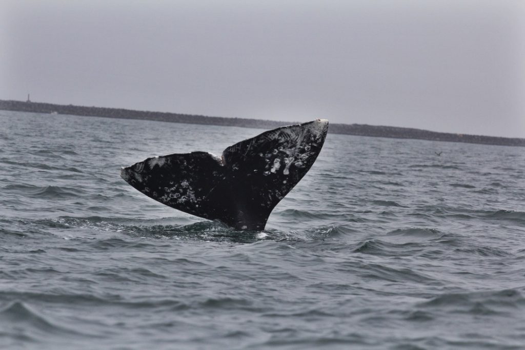
Gray whale fluke. Image captured under NOAA/NMFS permit #21678. Photo: L Hildebrand.

Final thoughts

Many unknowns still remain about the ENP and PCFG gray whale populations. During the ALJ hearing, both sides tried to deal with these unknowns. After reading testimony from both sides, it is clear to me that some of the unknowns still have not been reconciled. Ultimately, a lot of the questions circle back to the first one I posed above: Are the PCFG an independent stock? If there is independent population structure, then the proposed waiver put forth by NMFS would likely change. While NMFS has certainly taken the PCFG into account during the declarations of several experts at the ALJ hearing and has aired on the side of caution, the fact that the PCFG is considered part of the ENP might underestimate the impact that a resumption of the Makah hunt may have on the PCFG. As you can see, there are still many questions that should be addressed to make fully informed decisions on such an important ruling. While this research may take several years to obtain results, the data are within reach through synthesis and collaboration that will fill these critical knowledge gaps.

Literature cited

Calambokidis, J. C., J. Laake, and A. Pérez. 2017. Updated analysis of abundance and population structure of seasonal gray whales in the Pacific Northwest, 1996-2015. International Whaling Commission SC/A17/GW/05.

Frasier, T. R., S. M. Koroscil, B. N. White, and J. D. Darling. 2011. Assessment of population substructure in relation to summer feeding ground use in eastern North Pacific gray whale. Endangered Species Research 14:39-48.

Kirk, Ruth. 1986. Tradition and change on the Northwest Coast: the Makah, Nuu-chah-nulth, southern Kwakiutl and Nuxalk. University of Washington Press, Seattle.

Lang, A. R., D. W. Weller, R. LeDuc, A. M. Burdin, V. L. Pease, D. Litovka, V. Burkanov, and R. L. Brownell, Jr. 2011. Genetic analysis of stock structure and movements of gray whales in the eastern and western North Pacific. SC/63/BRG10.

Moore, J. E. 2019. Declaration in re: ‘Proposed Waiver and Regulations Governing the Taking of Eastern North Pacific Gray Whales by the Makah Indian Tribe’. Administrative Law Judge, Hon. George J. Jordan. Docket No. 19-NMFS-0001. RINs: 0648-BI58; 0648-XG584.

Schubert, D. J. 2019. Rebuttal testimony in re: ‘Proposed Waiver and Regulations Governing the Taking of Eastern North Pacific Gray Whales by the Makah Indian Tribe’. Administrative Law Judge, Hon. George J. Jordan. Docket No. 19-NMFS-0001. RINs: 0648-BI58; 0648-XG584.

Scordino, J. J., M. Gosho, P. J. Gearin, A. Akmajian, J. Calambokidis, and N. Wright. 2017. Individual gray whale use of coastal waters off northwest Washington during the feeding season 1984-2011: Implications for management. Journal of Cetacean Research and Management 16:57-69.

Villegas-Amtmann, S. 2019. Declaration in re: ‘Proposed Waiver and Regulations Governing the Taking of Eastern North Pacific Gray Whales by the Makah Indian Tribe’. Administrative Law Judge, Hon. George J. Jordan. Docket No. 19-NMFS-0001.

Weller, D. W., S. Bettridge, R. L. Brownell, Jr., J. L. Laake, J. E. Moore, P. E. Rosel, B. L. Taylor, and P. R. Wade. 2013. Report of the National Marine Fisheries Service Gray Whale Stock Identification Workshop. NOAA-TM-NMFS-SWFSC-507.

Yates, C. 2019a. Declaration in re: ‘Proposed Waiver and Regulations Governing the Taking of Eastern North Pacific Gray Whales by the Makah Indian Tribe’. Administrative Law Judge, Hon. George J. Jordan. Docket No. 19-NMFS-0001. RINs: 0648-BI58; 0648-XG584.

Yates, C. 2019b. Fifth declaration in re: ‘Proposed Waiver and Regulations Governing the Taking of Eastern North Pacific Gray Whales by the Makah Indian Tribe’. Administrative Law Judge, Hon. George J. Jordan. Docket No. 19-NMFS-0001. RINs: 0648-BI58; 0648-XG584.

The complex relationship between behavior and body condition

Clara Bird, Masters Student, OSU Department of Fisheries and Wildlife, Geospatial Ecology of Marine Megafauna Lab

Imagine that you are a wild foraging animal: In order to forage enough food to survive and be healthy you need to be healthy enough to move around to find and eat your food. Do you see the paradox? You need to be in good condition to forage, and you need to forage to be in good condition. This complex relationship between body condition and behavior is a central aspect of my thesis.

One of the great benefits of having drone data is that we can simultaneously collect data on the body condition of the whale and on its behavior. The GEMM lab has been measuring and monitoring the body condition of gray whales for several years (check out Leila’s blog on photogrammetry for a refresher on her research). However, there is not much research linking the body condition of whales to their behavior. Hence, I have expanded my background research beyond the marine world to looked for papers that tried to understand this connection between the two factors in non-cetaceans. The literature shows that there are examples of both, so let’s go through some case studies.

Ransom et al. (2010) studied the effect of a specific type of contraception on the behavior of a population of feral horses using a mixed model. Aside from looking at the effect of the treatment (a type of contraception), they also considered the effect of body condition. There was no difference in body condition between the treatment and control groups, however, they found that body condition was a strong predictor of feeding, resting, maintenance, and social behaviors. Females with better body condition spent less time foraging than females with poorer body condition. While it was not the main question of the study, these results provide a great example of taking into account the relationship between body condition and behavior when researching any disturbance effect.

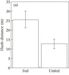
While Ransom et al. (2010) did not find that body condition affected response to treatment, Beale and Monaghan (2004) found that body condition affected the response of seabirds to human disturbance. They altered the body condition of birds at different sites by providing extra food for several days leading up to a standardized disturbance. Then the authors recorded a set of response variables to a disturbance event, such as flush distance (the distance from the disturbance when the birds leave their location). Interestingly, they found that birds with better body condition responded earlier to the disturbance (i.e., when the disturbance was farther away) than birds with poorer body condition (Figure 1). The authors suggest that this was because individuals with better body condition could afford to respond sooner to a disturbance, while individuals with poorer body condition could not afford to stop foraging and move away, and therefore did not show a behavioral response. I emphasize behavioral response because it would have been interesting to monitor the vital rates of the birds during the experiment; maybe the birds’ heart rates increased even though they did not move away. This finding is important when evaluating disturbance effects and management approaches because it demonstrates the importance of considering body condition when evaluating impacts: animals that are in the worst condition, and therefore the individuals that are most vulnerable, may appear to be undisturbed when in reality they tolerate the disturbance because they cannot afford the energy or time to move away.

Figure 1. Figure showing flush distance of birds that were fed (good body condition) and unfed (poor body condition).

These two studies are examples of body condition affecting behavior. However, a study on the effect of habitat deterioration on lizards showed that behavior can also affect body condition. To study this effect, Amo et al. (2007) compared the behavior and body condition of lizards in ski slopes to those in natural areas. They found that habitat deterioration led to an increased perceived risk of predation, which led to an increase in movement speed when crossing these deteriorated, “risky”, areas. In turn, this elevated movement cost led to a decrease in body condition (Figure 2). Hence, the lizard’s behavior affected their body condition.

Figure 2. Figure showing the difference in body condition of lizards in natural and deteriorated habitats.

Together, these case studies provide an interesting overview of the potential answers to the question: does body condition affect behavior or does behavior affect body condition? The answer is that the relationship can go both ways. Ransom et al. (2004) showed that regardless of the treatment, behavior of female horses differed between body conditions, indicating that regardless of a disturbance, body condition affects behavior. Beale and Monaghan (2004) demonstrated that seabird reactions to disturbance differed between body conditions, indicating that disturbance studies should take body condition into account. And, Amo et al. (2007) showed that disturbance affects behavior, which consequently affects body condition.

Looking at the results from these three studies, I can envision finding similar results in my gray whale research. I hypothesize that gray whale behavior varies by body condition in everyday circumstances and when the whale is disturbed. Yet, I also hypothesize that being disturbed will affect gray whale behavior and subsequently their body condition. Therefore, what I anticipate based on these studies is a circular relationship between behavior and body condition of gray whales: if an increase in perceived risk affects behavior and then body condition, maybe those affected individuals with poor body condition will respond differently to the disturbance. It is yet to be determined if a sequence like this could ever be detected, but I think that it is important to investigate.

Reading through these studies, I am ready and eager to start digging into these hypotheses with our data. I am especially excited that I will be able to perform this investigation on an individual level because we have identified the whales in each drone video. I am confident that this work will lead to some interesting and important results connecting behavior and health, thus opening avenues for further investigations to improve conservation studies.

References

Beale, Colin M, and Pat Monaghan. 2004. “Behavioural Responses to Human Disturbance: A Matter of Choice?” Animal Behaviour 68 (5): 1065–69. https://doi.org/10.1016/j.anbehav.2004.07.002.

Ransom, Jason I, Brian S Cade, and N. Thompson Hobbs. 2010. “Influences of Immunocontraception on Time Budgets, Social Behavior, and Body Condition in Feral Horses.” Applied Animal Behaviour Science 124 (1–2): 51–60. https://doi.org/10.1016/j.applanim.2010.01.015.

Amo, Luisa, Pilar López, and José Martín. 2007. “Habitat Deterioration Affects Body Condition of Lizards: A Behavioral Approach with Iberolacerta Cyreni Lizards Inhabiting Ski Resorts.” Biological Conservation 135 (1): 77–85. https://doi.org/10.1016/j.biocon.2006.09.020.

It all starts with the wind: The importance of upwelling

By Dawn Barlow, PhD student, OSU Department of Fisheries and Wildlife, Geospatial Ecology of Marine Megafauna Lab

The focus of my PhD research is on the ecology and distribution of blue whales in New Zealand. However, it has been a long time since I’ve seen a blue whale, and much of my time recently has been spent thinking about wind. What does wind matter to a blue whale? It actually matters a whole lot, because the wind drives an important biological process in many coastal oceans called upwelling. Wind blowing along shore, paired with the rotation of the earth, leads to a net movement of surface waters offshore (Fig. 1). As the surface water is pushed away, it is replaced by cold, nutrient-rich water from much deeper. When those nutrients become exposed to sunlight, they provide sustenance for the little planktonic lifeforms in the ocean, which in turn provide food for much larger predators including marine mammals such as blue whales. This “wind-to-whales” trophic pathway was coined by Croll et al. (2005), who demonstrated that off the West Coast of the United States, aggregations of whales could be expected downstream of upwelling centers, in concert with high productivity and abundant krill prey.

**Figure 1.** Graphic of the upwelling process, illustrating that when the wind blows along shore, surface waters are replaced by deeper water that is cold and nutrient rich. Source: NOAA

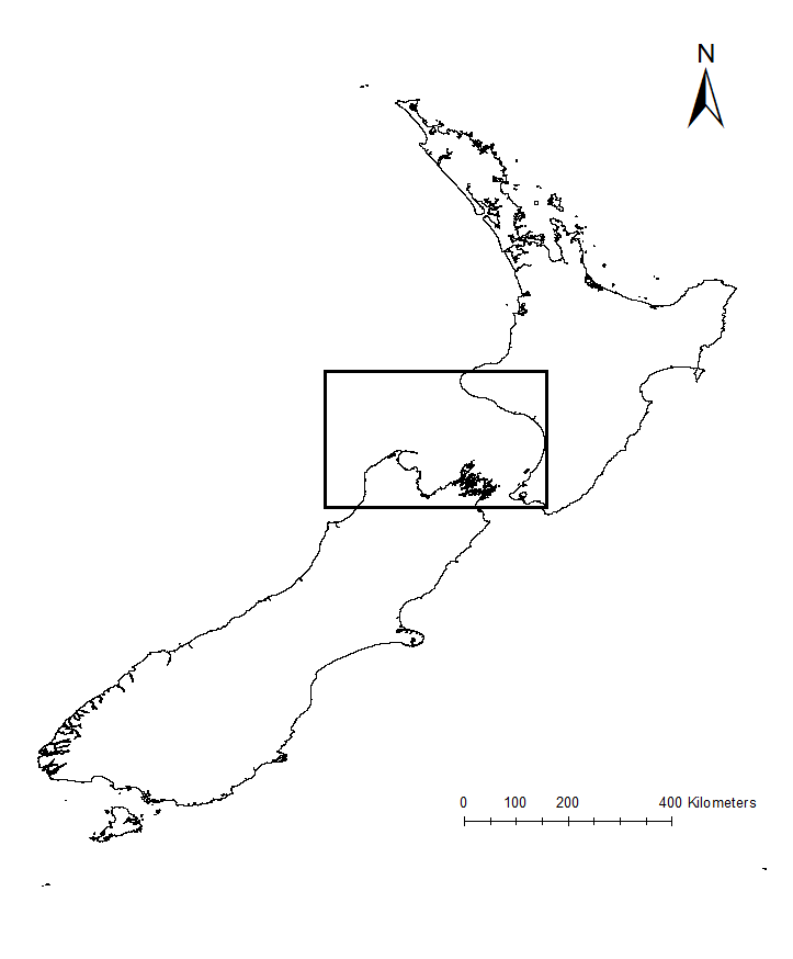
**Figure 2.** Map of New Zealand, with the South Taranaki Bight region (STB) denoted by the black box.

Much of what is understood today about upwelling comes from decades of research on the California Current ecosystem off the West Coast of the United States. Yet, the focus of my research is on an upwelling system on the other side of the world, in the South Taranaki Bight region (STB) of New Zealand (Fig. 2). In the case of the STB, westerly winds over Kahurangi Shoals lead to decreased sea level nearshore, forcing cold, nutrient rich waters to rise to the surface. The wind, along with the persistence of the Westland Current, then pushes a cold and productive plume of upwelled waters around Cape Farewell and into the STB (Fig. 3; Shirtcliffe et al. 1990).

**Figure 3.** Satellite image of the cold water plume in the South Taranaki Bight, indicative of upwelling. The origin of the upwelling at Kahurangi Shoals, Cape Farewell, and the typical path of the upwelling plume are denoted.

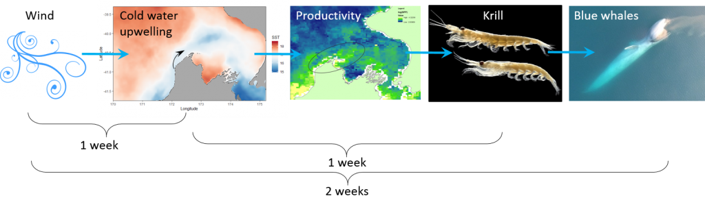
Through research conducted by the GEMM Lab over the years, we have demonstrated that blue whales utilize the STB region for foraging (Torres 2013, Barlow et al. 2018). Recent research on the oceanography of the STB region has further illuminated the mechanisms of this upwelling system, including the path and persistence of the upwelling plume in the STB across years and seasons (Chiswell et al. 2017, Stevens et al. 2019). However, the wind-to-whales pathway has not yet been described for this part of the world, and that is where the next section of my PhD research comes in. The whole system does not respond instantaneously to wind; the pathway from wind to whales takes time. But how much time is required for each step? How long after a strong wind event can we expect aggregations of feeding blue whales? These are some of the questions I am trying to tackle. For example, we hypothesize that some of the mechanisms and their respective lag times can be sketched out as follows:

**Figure 4.** The wind-to-whales trophic pathway, and hypothesized lags between steps.

All of these questions involve integrating oceanography, satellite imagery, wind data, and lag times, leading me to delve into many different analytical approaches including time series analysis and predictive modeling. If we are able to understand the lag times along this series of events leading to blue whale feeding opportunities, then we may be able to forecast blue whale occurrence in the STB based on the current wind and upwelling conditions. Forecasting with some amount of lead time could be a very powerful management tool, allowing for protection measures that are dynamic in space and time and therefore more effective in conserving this blue whale population and balancing human impacts.

**Figure 5.** A blue whale lunges on a patch of krill. The end of the wind-to-whales pathway. Drone piloted by Todd Chandler.

References:

Barlow DR, Torres LG, Hodge KB, Steel D, Baker CS, Chandler TE, Bott N, Constantine R, Double MC, Gill P, Glasgow D, Hamner RM, Lilley C, Ogle M, Olson PA, Peters C, Stockin KA, Tessaglia-hymes CT, Klinck H (2018) Documentation of a New Zealand blue whale population based on multiple lines of evidence. Endanger Species Res 36:27–40.

Chiswell SM, Zeldis JR, Hadfield MG, Pinkerton MH (2017) Wind-driven upwelling and surface chlorophyll blooms in Greater Cook Strait. New Zeal J Mar Freshw Res.

Croll DA, Marinovic B, Benson S, Chavez FP, Black N, Ternullo R, Tershy BR (2005) From wind to whales: Trophic links in a coastal upwelling system. Mar Ecol Prog Ser 289:117–130.

Shirtcliffe TGL, Moore MI, Cole AG, Viner AB, Baldwin R, Chapman B (1990) Dynamics of the Cape Farewell upwelling plume, New Zealand. New Zeal J Mar Freshw Res 24:555–568.

Stevens CL, O’Callaghan JM, Chiswell SM, Hadfield MG (2019) Physical oceanography of New Zealand/Aotearoa shelf seas–a review. New Zeal J Mar Freshw Res.

Torres LG (2013) Evidence for an unrecognised blue whale foraging ground in New Zealand. New Zeal J Mar Freshw Res 47:235–248.

Toxins in Marine Mammals: a Story

By: Alexa Kownacki, Ph.D. Student, OSU Department of Fisheries and Wildlife, Geospatial Ecology of Marine Megafauna Lab

As technology has developed over the past ten years, toxins in marine mammals have become an emerging issue. Environmental toxins are anything that can pose a risk to the health of plants or animals at a dosage. They can be natural or synthetic with varying levels of toxicity based on the organism and its physiology. Most prior research on the impacts toxins before the 2000s was conducted on land or in streams because of human proximity to these environments. However. with advancements in sampling methods, increasing precision in laboratory testing, and additional focus from researchers, marine mammals are being assessed for toxin loads more regularly.

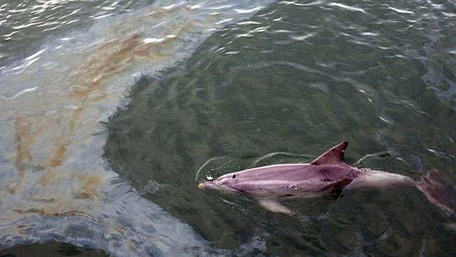
A dolphin swims through a diesel slick caused by a small oil spill in a port. (Image Source: The Ocean Update Blog)

Marine mammals live most of their lives in the ocean or other aquatic systems, which requires additional insulation for protection from both cold temperatures and water exposure. This added insulation can take the form of lipid rich blubber, or fur and hair. Many organic toxins are lipid soluble and therefore are more readily found and stored in fatty tissues. When an organic toxin like a polychlorinated biphenyl (PCB) is released into the environment from an old electrical transformer, it persists in sediments. As these sediments travel down rivers and into the ocean, these toxic substances slowly degrade in the environment and are lipophilic (attracted to fat). Small marine critters eat the sediment with small quantities of toxins, then larger critters eat those small critters and ingest larger quantities of toxins. This process is called biomagnification. By the time a dolphin consumes large contaminated fishes, the chemical levels may have reached a toxic level.

The process by which PCBs accumulate in marine mammals from small particles up to high concentrations in lipid layers. (Image Source: World Ocean Review)

Marine mammal scientists are teaming with biochemists and ecotoxicologists to better understand which toxins are more lethal and have more severe long-term effects on marine mammals, such as decreased reproduction rates, lowered immune systems, and neurocognitive delays. Studies have already shown that higher contaminant loads in dolphins cause all three of these negative effects (Trego et al. 2019). As a component of my thesis work on bottlenose dolphins I will be measuring contaminant levels of different toxins in blubber. Unfortunately, this research is costly and time-consuming. Many studies regarding the effects of toxins on marine mammals are funded through the US government, and this is where the public can have a voice in scientific research.

Rachel Carson examines a specimen from a stream collection site in the 1950s. (Image Source: Alfred Eisenstaedt/ The LIFE picture collection/ Getty Images.)

Prior to the 1960s, there were no laws regarding the discharge of toxic substances into our environment. When Rachel Carson published “Silent Spring” and catalogued the effects of pesticides on birds, the American public began to understand the importance of environmental regulation. Once World War II was over and people did not worry about imminent death due to wartime activities, a large portion of American society focused on what they were seeing in their towns: discharges from chemical plants, effluents from paper mills, taconite mines in the Great Lakes, and many more.

Discharge from a metallic sulfide mine collects in streams in northern Wisconsin. (Image Source: Sierra Club)

However, it was a very different book regarding pollutants in the environment that caught my attention – and that of a different generation and part of society – even more than “Silent Spring”. A book called “The Lorax”. In this 1972 children’s illustrated book by Dr. Seuss, a character called the Lorax “speaks for the trees”. The Lorax touches upon critical environmental issues such as water pollution, air pollution, terrestrial contamination, habitat loss, and ends with the poignant message, “Unless someone like you cared a whole awful lot, nothing is going to get better. It’s not.”

The original book cover for “The Lorax” by Dr. Seuss. (Image source: Amazon.com)

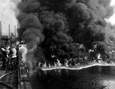
Within a decade, the US Environmental Protection Agency (EPA) was formed and multiple acts of congress were put in place, such as the National Environmental Policy Act, Clean Air Act, Clean Water Act, and Toxic Substances Control Act, with a mission to “protect human health and the environment.” The public had successfully prioritized protecting the environment and the government responded. Before this, rivers would catch fire from oil slicks, children would be banned from entering the water in fear of death, and fish would die by the thousands. The resulting legislation cleaned up our air, rivers, and lakes so that people could swim, fish, and live without fear of toxic substance exposures.

The Cuyahoga River on fire in June 1969 after oil slicked debris ignited. (Image Source: Ohio Central History).

Fast forward to 2018 and times have changed yet again due to fear. According to a Pew Research poll, terrorism is the number one issue that US citizens prioritize, and Congress and the President should address. The environment was listed as the seventh highest priority, below Medicare (“Majorities Favor Increased Spending for Education, Veterans, Infrastructure, Other Govt. Programs.”). With this societal shift in priorities, research on toxins in marine mammals may no longer grace the covers of the National Geographic, Science, or Nature, not for lack of importance, but because of the allocation of taxpayer funds and political agendas. Meanwhile, long-lived marine mammals will still be accumulating toxins in their blubber layers and we, the people, will need to care a whole lot, to save the animals, the plants, and ultimately, our planet.

The Lorax telling the reader how to save the planet. (Image Source: “The Lorax” by Dr. Seuss via the Plastic Bank)

Citations:

“Majorities Favor Increased Spending for Education, Veterans, Infrastructure, Other Govt. Programs.” Pew Research Center for the People and the Press, Pew Research Center, 11 Apr. 2019, www.people-press.org/2019/04/11/little-public-support-for-reductions-in-federal-spending/pp_2019-04-11_federal-spending_0-01-2/.

Marisa L. Trego, Eunha Hoh, Andrew Whitehead, Nicholas M. Kellar, Morgane Lauf, Dana O. Datuin, and Rebecca L. Lewison. Environmental Science & Technology 2019 53 (7), 3811-3822. DOI: 10.1021/acs.est.8b06487

PhD life: Pushing it to the extreme, and its wonders

By Leila S. Lemos, PhD candidate in Wildlife Sciences, Fisheries and Wildlife Department

I already started my countdown: 57 days until my PhD defense date! Being so close to this date brings me a lot of excitement about sharing with the community the results of the project I’ve been working on the past 4.5 years, and that I am really proud of. It also brings me lots of excitement when thinking about the new things that will come in my next phase of life. But even though I am excited, I’ve also been stressed, anxious and under depression. There is a mix of feelings rushing inside of me right now.

For those who don’t know me, I am originally from Rio de Janeiro, Brazil. I’ve been spending the last years far from my family, friends, language and culture. My favorite hobby always was to go to the beach and swim in the warm ocean. I would do that at least twice a week. Brazil is a tropical place and we can go to the beach all year round.

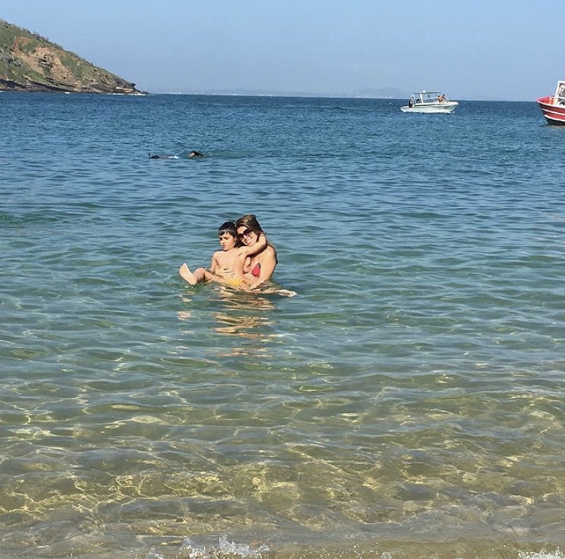
Me and my nephew in one of my favorite places in Brazil: Buzios, Rio de Janeiro.

Being in Oregon is really different. Oregon is gorgeous and I love it here, especially during the summer. However, the fall season brings the rain. Lots of rain, and it only stops around March. The absence of sun (and vitamin D) also contributes to depression. Even during the summer, I cannot swim in the ocean as the water is still really cold.

In addition to all of these factors, a PhD comes with classes, exams, fieldwork, research project, lots of reading and learning, manuscript writing, deadlines and great responsibilities. When you don’t have a scholarship or when it runs out (in my case), you also need to find a way to fund yourself until it finishes. Since last September I have been a teaching assistant for the university to cover my tuition and health insurance costs, and to earn a monthly stipend. The work never ends, and you always have more and more things to do.

A PhD is a full-time job, even if you are still technically a student. Actually, a PhD is a 24-hour job. Even if you are not working, you are thinking about your experiments and/or deadlines. Even if you are not awake, you are dreaming about it. You feel guilty all the time if you are doing things that are not related to your work.

But, it turns out I am not alone. The more I talk to people about the struggles, disappointments, anxiety, impostor syndrome, insomnia, depression, exhaustion of graduate school, the more I find that it is more common than I first thought. I have several friends facing the same problems right now.

I searched for some stats on this topic and I found a relatively recent study (Levecque et al. 2017) that evaluated the mental health of a sample of PhD students (N = 3659) from five different research discipline categories: sciences, biomedical sciences, applied sciences, humanities, and social sciences. PhD students were compared to other three groups: (1) highly educated individuals in the general population (N = 769), (2) highly educated employees (N = 592), and (3) higher education students (i.e., academic Bachelor, Master or Doctoral degree; N = 333). Research participants answered the web-based questionnaire that follows:

Table 1: Prevalence of common mental health problems in PhD students compared to three comparison groups.

Legend: RR: risk ratio adjusted for age and gender; CI: 95% confidence interval; GHQ2+: experienced at least two symptoms; GHQ3+: experienced at least three symptoms; GHQ4+: experienced at least four symptoms.
Source: Levecque et al. (2017)

It was alarming to me to see some of these results. Here are some of them:

A GHQ2+ score indicated psychological distress, and the prevalence was about twice as high in PhD students compared to the highly educated general population. PhD students were consistently more affected when compared to all of the other groups.
They found a significant relationship between psychological distress and the risk of having or developing a common psychiatric disorder (GHQ4+).
The odds of experiencing at least two psychological symptoms were 34% higher for female PhD students than for males.
No differences between scientific disciplines were found.

And here’s the funny thing: My PhD project researches stress in gray whales along the Oregon coast. I have been evaluating gray whale overall health by using different tools like photogrammetry, endocrinology and acoustics to monitor these individual whales. The more I read about stress and all the physiological response that occurs within the bodies of all vertebrates, the more I imagine it happening to me and all of the possible consequences. However, I do not consider myself a specialist on the theme yet, so I leave my mental health to a specialist. I have been seeing a psychiatrist and a psychologist and I have been learning that work-life balance is crucial, and it helps us maintain sanity. I have also been learning some “exercises” to help me with anxiety and impostor syndrome. This topic may not be an easy to talk about, but it is extremely important. If you are reading this and identify yourself, contact a professional who can help you. It has helped me.

Institutions should also increase their efforts to systematically map and monitor stressors and its outcomes in PhD students (Levecque et al. 2017). Identifying the problems and working towards solutions will benefit the institutions as students will do a better job.

Right now, I am just trying my best to achieve a work-life balance while I am still getting things done on time. All of my data has been analyzed and now I just need to write my chapters and prepare my defense presentation! It is hard to believe that in only 57 days I will be done.

I feel like I have succeeded in painting a grim picture of life as a PhD student. If you were thinking of going to grad school and now you have doubts about it, stop right there! Grad school is challenging, but it is not impossible. There are many things that will bring you joy in grad school like a successful fieldwork season, a successful experiment, a good grade on an exam you studied really hard for, a compliment from your advisor, a R code that is finally running correctly, or an accepted manuscript in a relevant journal.

By the way… I just had a manuscript of my first thesis chapter accepted for publication and I could not be happier:

Getting a PhD is hard, but it is also rewarding. Also, any path you take in your career will have pros and cons. What determines your success is your resilience and how you deal with the challenges that come. You may be asking if I would still do a PhD if I could go back in time, right? The answer is yes! Even though I have been facing many (personal) challenges I am really proud of my PhD project findings and am glad to be contributing to the knowledge and conservation of these amazing animals.

But please, if you see me around don’t forget:

References:

Costanza T. 2015. 10 memes relate to PhD students. Available at: https://www.siliconrepublic. com/careers/10-memes-relate-to-phd-students. Date of assess: 01/20/2020

Reddit. 2019. Made a meme for my boyfriend who’s doing his PhD. Available at: https://www.reddit.com/r/memes/comments/9fq2pq/made_a_meme_for_my_boyfriend_whos_doing_his_phd/. Date of assess: 01/20/2020

Levecque, K., F. Anseel, A. Beuckelaer, J. V. Heyden, and L. Gisle. 2017. Work organization and mental health problems in PhD students. Research Policy 46:868–879.

The teamwork of conservation science

Dr. Leigh Torres
PI, Geospatial Ecology of Marine Megafauna Lab, Marine Mammal Institute
Assistant Professor, Oregon Sea Grant, Department of Fisheries and Wildlife, Oregon State University

I have played on sports teams all my life – since I was four until present day. Mostly soccer teams, but a fair bit of Ultimate too. Teams are an interesting beast. They can be frustrating when communication breaks down, irritating when everyone is not on the same timeline, and disastrous if individuals do not complete their designated job. Yet, without the whole team we would never win. So, on top of the fun of competition, skill development, and exercise, playing on teams has always been part of the challenging and fulfilling process for me: everyone working toward the same goal – to win – by making the team fluid, complimentary, integrated, and ultimately successful.

I have come to learn that it is the same with conservation science.

A few of my teams through the ages, as player and coach. Some of my favorite people are on these teams, from 1981 to 2018.

Conservation efforts are often so complex, that it is practically impossible to achieve success alone. Forces driving the need for conservation typically include monetary needs/desires, social values, ecological processes, animal physiology, multi-jurisdictional policies, and human behavior. Each one of these forces alone is challenging to understand and takes expertise to comprehend the situation. Hence, building a well-functioning team is essential. Here’s a recent example from the GEMM Lab:

Since 2014 entanglements of blue, humpback and gray whales in fishing gear along the west coast of the USA have dramatically increased, particularly in Dungeness crab fishing gear. Many forces likely led to this increase, including increased whale population abundance, potential shifts in whale distributions, and changes in fishing fleet dynamics. While we cannot point a finger at one cause, many people and groups recognize that we cannot continue to let whales become entangled and killed at such high rates: whale populations would decline, fisheries would look bad in the public eye and potentially lose profits, whales have an intrinsic right to live in the ocean without being bycaught, and whales are an important part of the ecosystem that would deteriorate without them. In 2017, the Oregon Whale Entanglement Working Group was formed to bring stakeholders together that were concerned about this problem to discuss possible solutions and paths forward. I was lucky to be a part of this group, which also included members of the Dungeness crab fishery and commission, the Oregon Department of Fish and Wildlife (ODFW), other marine mammal scientists, and representatives of the American Cetacean Society, The Nature Conservancy, and a local marine gear supplier.

We met regularly over 2.5 years, and despite some hesitation at first about walking into a room of potentially disgruntled fishermen (I would be lying if I did not admit to this), after the first meeting I looked forward to every gathering. I learned an immense amount about the Dungeness crab fishery and how it operates, how ODFW manages the fishery and why, and what people do, don’t and need to know about whales in Oregon. Everyone agreed that reducing whale entanglements is needed, and a frequent approach discussed was to reduce risk by not setting gear where and when we expect whales to be. Yet, this idea flagged a very critical knowledge gap: We do not have a good understanding of whale distribution patterns in Oregon. Thus leading to the development of a highly collaborative research effort to describe whale distribution patterns in Oregon and identify areas of co-occurrence between whales and fishing effort to reduce the risk of entanglements. Sounds great, but a tough task to accomplish in a few short years. So, let me introduce the great team I am working with to make it all happen.

While I may know a few things about whales and spatial ecology, I don’t know too much about fisheries in Oregon. My collaboration with folks at ODFW, particularly Kelly Corbett and Troy Buell, has enabled this project to develop and go forward, and ultimately will lead to success. These partners provide feedback about how and where the fishery operates so I know where and when to collect data, and importantly they will provide the information on fishing effort in Oregon waters to relate to our generated maps of whale distribution. This spatial comparison will produce what is needed by managers and fishermen to make informed and effective decisions about where to fish, and not to fish, so that we reduce whale entanglement risk while still harvesting successfully to ensure the health and sustainability of our coastal economies.

So, how can we collect standardized data on whale distribution in Oregon waters without breaking the bank? I tossed this question around for a long time, and then I looked up to the sky and wondered what that US Coast Guard (USCG) helicopter was flying around for all the time. I reached out to the USCG to enquire, and proposed that we have an observer fly in the helicopter with them along a set trackline during their training flights. Turns out the USCG Sector North Bend and Columbia River were eager to work with us and support our research. They have turned out to be truly excellent partners in this work. We had some kinks to work out at the beginning – lots of acronyms, protocols, and logistics for both sides to figure out – but everyone has been supportive and pleasant to work with. The pilots and crew are interested in our work and it is a joy to hear their questions and see them learn about the marine ecosystem. And our knowledge of helicopter navigation and USCG duties has grown astronomically.

On the left is a plot of the four tracklines we survey for whales each month for two years aboard a US Coast Guard helicopter. On the right are some photos of us in action with our Coast Guard partners.

Despite significant cost savings to the project through our partnership with the USCG, we still need funds to support time, gear and more. And full credit to the Oregon Dungeness Crab Commission for recognizing the value and need for this project to support their industry, and stepping up to fund the first year of this project. Without their trust and support the project may not have got off the ground. With this support in our back pocket and proof of our capability, ODFW and I teamed up to approach the National Oceanographic and Atmospheric and Administration (NOAA) for funds to support the remaining years of the project. We found success through the NOAA Fisheries Endangered Species Act Section 6 Program, and we are now working toward providing the information needed to protect endangered and threatened whales in Oregon waters.

Despite our cost-effective and solid approach to data collection on whale occurrence, we cannot be everywhere all the time looking for whales. So we have also teamed up with Amanda Gladics at Oregon Sea Grant to help us with an important outreach and citizen science component of the project. With Amanda we have developed brochures and videos to inform mariners of all kinds about the project, objectives, and need for them to play a part. We are encouraging everyone to use the Whale Alert app to record their opportunistic sightings of whales in Oregon waters. These data will help us build and test our predictive models of whale distribution. Through this partnership we continue important conversations with fishermen from many fisheries about their concerns, where they are seeing whales, and what needs to be done to solve this complex conservation challenge.

Of course I cannot collect, process, analyze, and interpret all this data on my own. I do not have the skills or capacity for that. My partner in the sky is Craig Hayslip, a Faculty Research Assistant in the Marine Mammal Institute. Craig has immense field experience collecting data on whales and is the primary observer on the survey flights. Together we have navigated the USCG world and developed methods to collect our data effectively and efficiently (all within a tiny space flying over the ocean). In a few months we will be ¾ of the way through our data collection phase, which means data analysis will take over. For this phase I am bringing back a GEMM Lab star, Solene Derville, who recently completed her PhD. As the post-doc on the project, Solene will take the lead on the species distribution modeling and fisheries overlap analysis. I am looking forward to partnering with Solene again to compile multiple data sources on whales and oceanography in Oregon to produce reliable and accurate predictions of whale occurrence and entanglement risk. Finally I want to acknowledge our great partners at the Cascadia Research Collective (Olympia, WA) and the Cetacean Conservation and Genomics Lab (OSU, Marine Mammal Institute) who help facilitate our data collection, and conduct the whale photo-identification or genetic analyses to determine population assignment.

As you can see, even this one, smallish, conservation research project takes a diverse team of partners to proceed and ensure success. On this team, my position is sometimes a player, coach, or manager, but I am always grateful for these amazing collaborations and opportunities to learn. I am confident in our success and will report back on our accomplishments as we wrap up this important and exciting conservation science project.

A fin whale observed off the Oregon coast during one of our surveys aboard a US Coast Guard helicopter.

What are the ecological impacts of gray whale benthic feeding?

Clara Bird, Masters Student, OSU Department of Fisheries and Wildlife, Geospatial Ecology of Marine Megafauna Lab

Happy new year from the GEMM lab! Starting graduate school comes with a lot of learning. From skills, to learning about how much there is to learn, to learning about the system I will be studying in depth for the next few years. This last category has been the most exciting to me because digging into the literature on a system or a species always leads to the unearthing of some fascinating and surprising facts. So, for this blog I will write about one of the aspects of gray whale foraging that intrigues me most: benthic feeding and its impacts.

How do gray whales feed?

Gray whales are a unique species. Unlike other baleen whales, such as humpback and blue whales, gray whales regularly feed off the bottom of the ocean (Nerini, 1984). They roll to one side and swim along the bottom, they then suction up (by depressing their tongue) the sediment and prey, then the sediment and water is filtered out of the baleen. In fact, we use sediment streams, shown in Figure 1, as an indicator of benthic feeding behavior when analyzing drone footage (Torres et al. 2018).

*Figure 1. Screenshot of drone video showing sediment streaming from mouth of a whale after benthic feeding. Video taken under NOAA/NMFS permit #21678*

Locations of benthic feeding can be identified without directly observing a gray whale actively feeding because of the excavated pits that result from benthic feeding (Nerini 1984). These pits can be detected using side-scan sonar that is commonly used to map the seafloor. Oliver and Slattery (1985) found that the pits typically are from 2-20 m². In some of the imagery, consecutive neighboring pits are visible, likely created by one whale in series during a feeding event. Figure 2 shows different arrangements of pits.

*Figure 2. Different arrangements of pits created by feeding whales (Nerini 1984).*

Aside from how fascinating the behavior is, benthic feeding is also interesting because it has a large impact on the environment. Coming from a background of studying baleen whales that primarily feed on krill, I had not really considered the potential impacts of whale foraging other than removing prey from the environment. However, when gray whales feed, they excavate large areas of the benthic substrate that disturb and impact the habitat.

The impacts of benthic feeding

Weitkamp et al. (1992) conducted a study on gray whale benthic foraging on ghost shrimp in Puget Sound, WA, USA. This study, conducted over two years, focused on measuring the impact of benthic foraging by its effect on prey abundance. They found that the standing stock of ghost shrimp within a recently excavated pit was two to five times less than that outside the pit, and that 3100 to 5700 grams of shrimp can be removed per pit. From aerial surveys they estimated that within one season feeding gray whales created between 2700 and 3200 pits. Using these values, they calculated that 55 to 79% of the standing stock of ghost shrimp was removed each season by foraging gray whales. Interestingly, they found that the shrimp biomass within an excavated pit recovered within about two months.

Oliver and Slattery (1985) also found a recovery period of about 2 months per pit in their study on the effect of gray whale benthic feeding on the prey community in the Bering Sea. They sampled prey within and outside feeding excavations, both actual whale pits and man-made, to test the response of the benthic community to the disturbance of a feeding event. They found that after the initial feeding disturbance, the excavated area was rapidly colonized by scavenging lysianassid amphipods, which are small (10 mm) crustaceans that typically eat dead organic material. These amphipods rushed in and attacked the organisms that were injured or dislodged by the whale feeding event, typically small crustaceans and polychaete worms. Within hours of the whale feeding event, these amphipods had dispersed and a different genre of scavenging lysianassid amphipods slowly invaded the excavated pit further and stayed much longer. After a few days or weeks these pits collected and trapped organic debris that attracted more colonists. Indeed, they found that the number of colonists remained elevated within the excavated areas for over two months.

Notably, these results on how the disturbance of gray whale benthic feeding changes sediment composition support the idea that this foraging behavior maintains the sand substrate and therefore helps to maintain balanced levels of benthic dwelling amphipods, their primary source of prey in this study area (Johnson and Nelson, 1984). Gray whales scour the sea floor when they feed and this process leads to the resuspension of lots of sediments and nutrients that would otherwise remain on the seafloor. Therefore, while this feeding may seem like a violent disturbance, it may in fact play a large role in benthic productivity (Johnson and Nelson, 1984; Oliver and Slattery, 1985).

These ecosystem impacts of gray whale benthic feeding I have described above demonstrate the various stages of invaders after a feeding disturbance, and the process of succession. Succession is the ecological process of how a community structure builds and grows. Primary succession is when the structure grows from truly nothing and secondary succession occurs after a disturbance, such as a fire. In secondary succession, there are typically pioneer species that first appear and then give way to other species and a more complex community eventually emerges. Succession is well documented in many terrestrial studies after disturbance events, and the processes of secondary succession is very important to community ecology and resilience.

Since gray whale benthic foraging does not impact an entire habitat all at once, the process is not perfectly comparable to secondary succession in terrestrial systems. Yet, when thinking about the smaller scale, another example of succession in the marine environment takes place at a whale fall. When a whale dies and sinks to the ocean floor, a small ecosystem emerges. Different organisms arrive at different stages to scavenge different parts of the carcass and a food web is created around it.

To me the impacts of gray whale benthic feeding are akin to both terrestrial disturbance events and whale falls. The excavation serves as a disturbance, and through secondary succession the habitat is refreshed via stages of different species colonization until the system eventually returns to the pre-disturbance levels. However, like a whale fall the feeding event leaves behind injured or displaced organisms that scavengers consume; in fact seabirds are known to take advantage of benthic invertebrates that are brought to the surface by a gray whale feeding event (Harrison, 1979).

So much of our research is focused on questions about how the changing environment impacts our study species and not the other way around. This venture into the literature has provided me with an important reminder to think about flipping the question. I have enjoyed starting 2020 with a reminder of how cool gray whales are, and that while a disturbance can initially be thought of as negative, it may actually bring about important, and positive, change.

References

Nerini, Mary. 1984. “A Review of Gray Whale Feeding Ecology.” In The Gray Whale: Eschrichtius Robustus, 423–50. Elsevier Inc. https://doi.org/10.1016/B978-0-08-092372-7.50024-8.

Oliver, J. S., and P. N. Slattery. 1985. “Destruction and Opportunity on the Sea Floor: Effects of Gray Whale Feeding.” Ecology 66 (6): 1965–75. https://doi.org/10.2307/2937392.

Torres, Leigh G., Sharon L. Nieukirk, Leila Lemos, and Todd E. Chandler. 2018. “Drone up! Quantifying Whale Behavior from a New Perspective Improves Observational Capacity.” Frontiers in Marine Science 5 (SEP). https://doi.org/10.3389/fmars.2018.00319.

Weitkamp, Laurie A, Robert C Wissmar, Charles A Simenstad, Kurt L Fresh, and Jay G Odell. 1992. “Gray Whale Foraging on Ghost Shrimp (Callianassa Californiensis) in Littoral Sand Flats of Puget Sound, USA.” Canadian Journal of Zoology 70 (11): 2275–80. https://doi.org/10.1139/z92-304.

Johnson, Kirk R., and C. Hans Nelson. 1984. “Side-Scan Sonar Assessment of Gray Whale Feeding in the Bering Sea.” Science 225 (4667): 1150–52.

Harrison, Craig S. 1979. “The Association of Marine Birds and Feeding Gray Whales.” The Condor 81 (1): 93. https://doi.org/10.2307/1367866.

GEMM Lab 2019: A Year in the Life

By Lisa Hildebrand, MSc student, OSU Department of Fisheries & Wildlife, Geospatial Ecology of Marine Megafauna Lab

Another year has come and gone, and with the final days of 2019 upon us, it is fulfilling to look back and summarize all of the achievements in the GEMM Lab this year. So, snuggle up with your favorite holiday drink and enjoy our recap of 2019!

We wrapped up two intense but rewarding gray whale field seasons this summer. Our project investigating the health of Pacific Coast Feeding Group (PCFG) gray whales through fecal hormone and body condition sampling in the context of ocean noise went into its fourth year, while the Port Orford project where we track whales and prey at a very fine-scale celebrated its wood anniversary (five years!). The dedication and hard work of lots of people to help us collect our data meant that we were able to add a considerable amount of samples to our growing gray whale datasets. Our trusty red RHIB Ruby zipped around the Pacific and enabled us to collect 58 fecal samples, fly the drone 102 times, undertake 105 GoPro drops and record 141 gray whale sightings. Our Newport crew was a mix of full-time GEMMers (Leigh, Todd, Dawn, Leila, Clara, and myself) as well as part-time summer GEMMers (Ale, Sharon, and Cassy). Further south in Port Orford, my team of undergraduate and high school students and I had an interesting field season. We only encountered four different individuals (Buttons, Glacier, Smudge, and Primavera), however saw them repeatedly throughout the month of August, resulting in as many as 15 tracklines for one individual. Furthermore, we collected 249 GoPro drops and 248 zooplankton net samples.

Leila taking photos of gray whales from Ruby’s bow pulpit. Photo: Leigh Torres

The GEMM Lab’s fieldwork was not just restricted to gray whales. After last year’s successes aboard the NOAA ship Bell M. Shimada, Alexa and Dawn both boarded the ship again this year as marine mammal observers for the May and September cruises, respectively. They spied humpback, blue, sperm, and fin whales, as well as many dolphins and seabirds, adding to the GEMM Lab’s growing database of megafauna distribution off the Oregon coast.

Alexa observing on the R/V Shimada in May 2019, all bundled up. Image Photo: Alexa Kownacki

After winning the prestigious L’Oréal-UNESCO For Women in Science fellowship and the inaugural Louis Herman Scholarship, GEMM Lab grad Solène Derville lead her first research cruise aboard the French R/V Alis. She and her team conducted line transect surveys and micronekton/oceanographic sampling over several seamounts to try to solve the mystery of why humpbacks hang out there. We are also very excited to announce that Solène will be returning to the GEMM Lab as a post-doc in 2020! She will be creating distribution models of whales off the coast of Oregon with the data collected by Leigh during helicopter flights with the US Coast Guard. The primary aim of this work is to identify potential whale hotspots in an effort to avoid spatial overlap with fisheries gear and reduce entanglement risk.

Solène soaking wet after spending several hours observing cetaceans and seabirds on R/V Alis. Photo: Jérôme Jambou

Switching the focus from marine mammals to seabirds, Rachael has had an extremely busy year of field work all across the globe. She island-hopped from Midway (Hawaiian Northwest island) to the Falkland Islands in the first half of the year, and is currently overwintering on South Georgia, where she will be until end of February. Rachael is tracking albatross at all three locations by tagging individual birds to understand movements relative to fishing vessels and flight energetics.

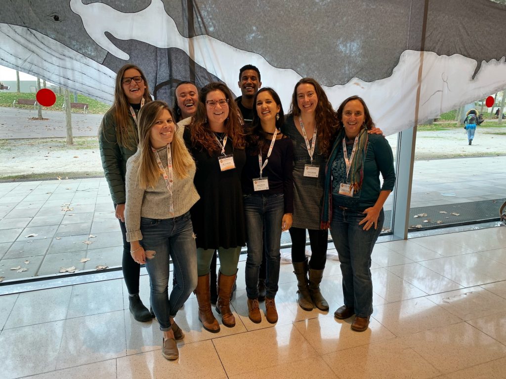
Besides several field efforts, the GEMM Lab was also busy disseminating our research and findings to various audiences. Our conferences kicked off in late February when Leigh and Rachael both flew to Kauai to present at the Pacific Seabird Group’s 46^th Annual Meeting. In the spring, Leila, Dawn, Alexa, Dom, and myself drove to Seattle where the University of Washington hosted the Northwest Student Society of Marine Mammalogy chapter meeting and we all gave talks. Additionally, the Fisheries & Wildlife grad students in the lab also presented at the department’s annual Research Advances in Fisheries, Wildlife, and Ecology conference. Later in the year, Dom and I attended the State of the Coast conference where Dom was invited to participate in a panel about the holistic approaches to management in the nearshore while I presented a poster on preliminary findings of my Master’s thesis. Most recently, the entire GEMM Lab (bar Rachael) flew to Barcelona to present at the World Marine Mammal Conference (WMMC).

GEMM Lab at the WMMC. Photo: Karen Lohman

Our science communication and outreach efforts were not just restricted to conferences though. Over the course of this year, the GEMM Lab supervised a total of 10 undergraduate and high school interns that assisted in a variety of ways (field and/or lab work, data analyses, independent projects) on a number of projects going on in the lab. Leigh and Dawn boarded the R/V Oceanus in the fall to co-lead a STEM research cruise aimed at providing high school students and teachers hands-on marine research. Dawn and I were guests on Inspiration Dissemination, a live radio show run by graduate students about graduate research going on at OSU. Our weekly blog, now in its fifth year, reached its highest viewership with a total of 14,814 views this year!

The GEMMers were once again prolific writers too! The 13 new publications in 10 scientific journals include contributions from Leigh (7), Rachael (6), Solène (2), Dawn (2), and Leila (1). Scroll down to the end of the post to see the list.

Academic milestones were also reached by several of us. Most notably and recently, Dom successfully defended his Master’s thesis this past week – congratulations Dom!! Unsurprisingly, he already has a job lined up starting in January as a Science Officer with the California Ocean Science Trust. Dom is the 6^th GEMM Lab graduate, which after just five years of the GEMM Lab existing is a huge testament to Leigh as an advisor. Leila, who is in the 4^th year of her PhD, anticipates finishing this coming March. We also had three successful research reviews – I met with my committee in late March to discuss my Master’s proposal, while Alexa and Dawn met with their committees in the summer to review their PhD proposals. All three reviews were fruitful and successful. And we want to highlight the success of a GEMM Lab grad, Florence Sullivan, who started a job in Maui with the Pacific Whale Foundation in September as a Research Analyst.

Dom during his MS seminar. Photo: Leila Lemos

Leigh was recognized for her expertise in gray whale ecology and was appointed to the IUCN Western Gray Whale Advisory Panel (WGWAP). The western gray whales are a critically endangered population. At one point in the 1960s, the population was so scarce that they were believed to have been extinct. While this concern did not prove to be the case, the population still is not doing well, which is why the IUCN formed WGWAP to provide advice on the conservation of the western gray whales. Leigh was appointed to the panel this year and traveled to Switzerland and Russia for meetings.

Clara aboard Ruby on her first day of gray whale field work in Oregon. Photo: Leigh Torres

We are excited about a new addition to the lab. Clara Bird started her MS in Wildlife Science in the Department of Fisheries & Wildlife this fall. She jumped straight into field work when she came in early September and got a taste of the Pacific. Clara joins us from the Duke University where she did her undergraduate degree and worked for the past year in their Marine Robotics and Remote Sensing Lab. Clara is digging into the gray whale drone footage collected over the last four field seasons and scrutinize them from a behavioral point of view.

If you are reading this post, we would like to say that we really appreciate your support and interest in our work! We hope you will continue to join us on our journeys in 2020. Until then, happy holidays from the GEMM Lab!

GEMM Lab at the beginning of June with some permanents GEMMs and some temporary summer GEMM helpers.

Barlow, D. R., M. Fournet, and F. Sharpe. 2019. Incorporating tides into the acoustic ecology of humpback whales. Marine Mammal Science 35:234-251.

Barlow, D. R., A. L. Pepper, and L. G. Torres. 2019. Skin deep: an assessment of New Zealand blue whale skin condition. Frontiers in Marine Science doi.org/10.3389/fmars.2019.00757.

Baylis, A. M. M., R. A. Orben, A. A. Arkhipkin, J. Barton, R. L. Brownell Jr., I. J. Staniland, and P. Brickle. 2019. Re-evaluating the population size of South American fur seals and conservation implications. Aquatic Conservation: Marine and Freshwater Ecosystems 29(11):1988-1995.

Baylis, A. M. M., M. Tierney, R. A. Orben, et al. 2019. Important at-sea areas of colonial breeding marine predators on the southern Patagonian Shelf. Scientific Reports 9:8517.

Cockerham, S., B. Lee, R. A. Orben, R. M. Suryan, L. G. Torres, P. Warzybok, R. Bradley, J. Jahncke, H. S. Young, C. Ouverney, and S. A. Shaffer. 2019. Microbial biology of the western gull (Larus occidentalis). Microbial Ecology 78:665-676.

Derville, S., L. G. Torres, R. Albertson, O. Andrews, C. S. Baker, P. Carzon, R. Constantine, M. Donoghue, C. Dutheil, A. Gannier, M. Oremus, M. M. Poole, J. Robbins, and C. Garrigue. 2019. Whales in warming water: assessing breeding habitat diversity and adaptability in Oceania’s changing climate. Global Change Biology 25(4):1466-1481.

Derville, S., L. G. Torres, R. Dodémont, V. Perard, and C. Garrigue. 2019. From land and sea, long-term data reveal persistent humpback whale (Megaptera novaeangliae) breeding habitat in New Caledonia. Aquatic Conservation: Marine and Freshwater Ecosystems 29(10):1697-1711.

Fleischman, A. B., R. A. Orben, N. Kokubun, A. Will, R. Paredes, J. T. Ackerman, A. Takahashi, A. S. Kitaysky, and S. A. Shaffer. 2019. Wintering in the western Subantarctic Pacific increases mercury contamination of red-legged kittiwakes. Environmental Science & Technology 53(22):13398-13407.

Holdman, A. K., J. H. Haxel, H. Klinck, and L. G. Torres. 2019. Acoustic monitoring reveals the times and tides of harbor porpoise (Phocoena phocoena) distribution off central Oregon, U.S.A. Marine Mammal Science 35:164-186.

Kroeger, C., D. E. Crocker, D. R. Thompson, L. G. Torres, P. Sagar, and S. A. Shaffer. 2019. Variation in corticosterone levels in two species of breeding albatrosses with divergent life histories: responses to body condition and drivers of foraging behavior. Physiological and Biochemical Zoology 92(2):223:238.

Loredo, S. A., R. A. Orben, R. M. Suryan, D. E. Lyons, J. Adams, and S. W. Stephensen. 2019. Spatial and temporal diving behavior of non-breeding common murres during two summers of contrasting ocean conditions. Journal of Experimental Biology and Ecology 517:13-24.

Monteiro, F., L. S. Lemos, J. Fulgêncio de Moura, R. C. C. Rocha, I. Moreira, A. P. Di Beneditto, H. A. Kehrig, I. C. A. C. Bordon, S. Siciliano, T. D. Saint’Pierre, and R. A. Hauser-Davis. 2019. Subcellular metal distributions and metallothionein associations in rough-toothed dolphins (Steno bredanensis) from southeastern Brazil. Marine Pollution Bulletin 146:263-273.

Orben, R. A., A. B. Fleischman, A. L. Borker, W. Bridgeland, A. J. Gladics, J. Porquez, P. Sanzenbacher, S. W. Stephensen, R. Swift, M. W. McKown, and R. M. Suryan. 2019. Comparing imaging, acoustics, and radar to monitor Leach’s storm-petrel colonies. PeerJ 7:e6721.

Yates, K. L., …, L. G. Torres, et al. 2019. Outstanding challenges in the transferability of ecological models. Trends in Ecology & Evolution 33(10):790-802.

Flying halfway around the world to learn about marine mammals from around the world!

By Lisa Hildebrand, MSc student, OSU Department of Fisheries & Wildlife, Geospatial Ecology of Marine Megafauna Lab

The GEMM Lab is back from Barcelona after attending the World Marine Mammal Conference last week and it sure was a week to remember! Not only did every GEMM member present some aspect of their research at the conference (either as a poster, speed or full-length talk) but some of us also attended workshops, scheduled meetings with collaborators, new & old, and we certainly all learned a lot of new information about what is going on in marine mammalogy across the globe. Having had a few days now to reflect upon the intense four days spent at the conference, we want to highlight the talks that we each personally thought were some of the most interesting and exciting.

“Double Drone Drama” was the alliterative title of Héloïse Frouin-Mouy‘s talk about using two drones to collect simultaneous visual and underwater acoustic behavioral data of gray whales in Baja California, Mexico. While there were many talks during the week that discussed incorporating drones, also known as unmanned aerial vehicles (UAVs), into marine mammal research, this project was potentially the only one that discussed using two simultaneously. One drone collected visual aerial observations while the other obtained close-range passive acoustic measurements with an underwater recording hydrophone to better understand the behavioral contexts of call generation. Froiun-Mouy and her team detected call-type-specific source levels relative to behavior state through this dual-approach. For example, they were able to estimate the acoustic source levels of bubble-blasts produced by gray whales, and the double drone action recorded a variety of calls. Using two or more UAVs can provide a more integrated snapshot into the animal vocalization context, and it will be interesting to see whether this method is applied elsewhere on a variety of whale species.

Tara Sayuri Whitty. Source: UCSD Aquarium.

Tara Sayuri Whitty discussed her doctoral research focused on understanding the mental models of local, artisanal fishing communities at the heart of the vaquita conservation efforts. The vaquita has experienced rapid population declines due primarily to bycatch in gillnet fisheries from legal local gillnet fisheries and the illegal totoaba fishery. With the sole intent of preventing bycatch, gillnets were banned for legal practice, but the illegal totoaba fishery continued, as did vaquita bycatch. Whitty conducted interviews to understand the mental models and perceptions of local fishing communities towards officials and conservationists regarding the gillnet band. She discovered that these conservation efforts have not only failed to prevent vaquita bycatch, but they have now pitted conservationists against local communities because an important aspect of their livelihoods is now banned. This misstep and lack of trust with the community now threatens future conservation and recovery progress for the vaquita and highlights the need to collaborate and engage with local communities early and often when such efforts are so closely tied to human well-being.

Pauline Goulet, a PhD student in the Sea Mammal Research Unit at the University of St. Andrews, presented findings obtained from a novel sonar tag deployed on southern elephant seals (SES) in the Kerguelen Islands and Peninsula Valdes. Gaining insight into predator-prey interactions is critical to understanding the ecology of marine mammals as they live in dynamic and vast environments where prey is patchy. Collecting in-situ prey information is difficult, and in some cases impossible, due to the remote locations where marine mammals forage and it is not being feasible to follow individuals around continuously to collect prey samples at every foraging event. In an attempt to overcome this universal challenge to marine mammal research, Goulet and her collaborators decided to mimic the experts in prey detection and visualization from a distance in the marine environment – echolocating odontocetes. By equipping conventional DTAGs with a 1.5 MHz single beam sonar with a 6 m detection range, Goulet was able to identify whether SES were pursuing individual fish or large schools of fish. Additionally, by also analyzing the accelerometer data, she could document whether prey capture attempts were successful or not, and link these results to the body condition of individual SES (inferred from the horizontal distance an individual traveled during drift dives, whereby a longer horizontal distance in the same period of time suggested that the individual had gained weight and was now heavier). It was ingenious to see researchers utilize a biological trait that evolved millions of years ago in certain marine mammal predators to better understand the ecology of another marine mammal predator.

A trio of talks given by Kristi Fazioli, Valeria Paz, and Shauna McBride-Kebert, in the ‘Habitat and Distribution II’ session, discussed responses of coastal bottlenose dolphins to hurricanes in the Gulf of Mexico (GoM). Besides continuing to be an area of interest in conservation after the Deepwater Horizon oil spill, the GoM frequently experiences hurricanes and other strong storm systems that cause extensive flooding events annually. Hence, dolphins along the GoM coast experience a large outflow of freshwater after severe precipitation, leading to low salinity events. Both Fazioli and Paz hypothesized that these changes in environmental conditions can create health problems to the dolphins.

Bottlenose dolphin underwater in the Gulf of Mexico. Source: Mike Heithaus.

Fazioli investigated encounter rates and skin conditions of bottlenose dolphins after Hurricane Harvey. She found that, in 2017, the encounter rates in her study area decreased, while skin lesions increased (Christina Toms, unpublished work, expected Spring 2020). Skin lesions are known to occur at higher rates after exposure to freshwater and even though they persist for some time, they eventually do heal. After less than two years, preliminary data suggest that these dolphins have returned to their original distributions in the study area. Paz’s study in Shark Bay Estuary examined different environmental drivers of dolphin distribution following Hurricane Irma. She found that dissolved oxygen, salinity, and temperature were the primary dynamic, environmental drivers of distribution following a major hurricane. Lastly, McBride’s species distribution models of bottlenose dolphins in response to severe flooding concluded that depth, slope, latitude, longitude, season, and dissolved oxygen all contributed in different percentages to distribution.

Marta Guerra presented findings from her PhD research at the University of Otago in New Zealand on the ecology and distribution of sperm whales in New Zealand. Kaikoura canyon is a region utilized by sperm whales for foraging, and Marta’s research highlighted marked differences in their distribution between the summer and winter, likely reflective of the sperm whales switching their target prey items seasonally. In the middle of their data collection period, a very intense earthquake struck the region in 2016, causing a canyon-flushing event that altered the canyon ecosystem. The sperm whales responded to this extreme event by altering their distribution away from the areas most affected by the earthquake, demonstrating that these marine predators respond to environmental shifts in the ecosystem they depend on at multiple scales.

On the final day of the conference, David Wiley gave a talk entitled “First documentation of coordinated bottom-feeding by humpback whales”. Using footage from tags containing a suite of sensors and video cameras, Wiley and colleagues observed humpback whales feeding on sand lace in the Stellwagen Bank National Marine Sanctuary. Sand lace are a species of fish that frequently burrow in the sand in an attempt to avoid capture by predators looking for their next meal. Humpback whales in the area have been observed with lacerations and scars along their mouths, originally leading to the hypothesis that whales were bottom-feeding. However, it was never known whether whales compete or cooperate when exploiting this resource and what the actual mechanics of this feeding behavior look like. The tag data revealed that groups of 3-4 individuals work together to approach the seafloor in a star-shape formation and when they get close enough, the sand lace emerge from the sand (probably an escape response to the approaching vibrations created by large whales) only to be engulfed by the humpbacks who are poised directly above them with wide-open mouths. Not only did the video footage reveal that individuals are so close together that their rostrums are almost touching, but Wiley and team were able to determine that whales perform their behavior usually within the same group of 3-4 individuals and that the orientation of each individual within the star-formation remains the same almost every time. This talk was so enjoyable because it was a reminder of how little we still know about marine mammals and provided a moment of audible awe and surprise throughout the room.

Share this:

Share this:

References

Share this:

Share this:

Share this:

Share this:

Share this:

How do gray whales feed?

The impacts of benthic feeding

References

Share this:

Share this:

Share this: