By Lindsay Wickman, Postdoctoral Scholar, Oregon State University Department of Fisheries, Wildlife, and Conservation Sciences, Geospatial Ecology of Marine Megafauna Lab
Previously on our blog, we mentioned the concerning rise of humpback whale (Megaptera novaeangliae) entanglement in fishing gear on the US West Coast (see here and here). Gaining an improved understanding of the rate of entanglement and risk factors of humpback whales in Oregon are primary aims of the GEMM Lab’s SLATE and OPAL projects. In this post, I will discuss some reasons why whales get entangled. With whales generally regarded as intelligent, it is understandable to wonder why whales are unable to avoid these underwater obstacles.
Figure 1. Wrapping scars like these at the base of the flukes indicate this humpback whale was previously entangled. Photo taken under NOAA/NMFS permit #21678 to John Calambokidis.
Fishing lines are hard to detect underwater
Water clarity, depth, and time of day can all influence how visible a fishing line is underwater. Since baleen whales lack the ability to discriminate color (Levenson et al., 2000; Peichl et al. 2001), the brightly colored yellow and red ropes that make it easier for fishermen to find their gear make it harder for whales to see it underwater. White or black ropes may stand out better for whales (Kot et al., 2012), but there’s not enough evidence yet to suggest they reduce entanglement rates.
Whales have excellent hearing, but this may still not be enough to ensure detection of underwater ropes. Even if whales can hear water currents flowing over the rope, this noise can easily be masked by other sounds like weather, surf, and passing boats. Fishing gear also has a weak acoustic signature (Leatherwood et al., 1977), or it may be at a frequency not heard by whales. So even though whales produce and listen for sounds to help locate prey (Stimpert et al., 2007) and communicate, any sound produced by fishing lines may not be sufficient to alert whales to its presence.
There are very few studies that examine the behavior of whales around fishing gear, but a study of minke whales (Balaenoptera acutorostrata) by Kot et al. (2017) provides an exception. Researchers observed whales slowing down as they approached their test gear, and speeding up once they were past it (Kot et al., 2017). While the scope of the study was too small to generalize about whales’ ability to detect fishing gear, it does suggest whales can detect fishing gear, at least some of the time. There is also likely some individual variation in this skillset. Less experienced, juvenile humpback whales, for example, may be at a higher risk of entanglement than adults (Robbins, 2012).
Distracted driving?
Just like distracted drivers are more likely to crash when texting or eating, whales may be more likely to get entangled when they are preoccupied with behaviors like feeding or socializing.
Evidence suggests feeding is especially risky for entanglement. An analysis of entanglements in the North Atlantic found that almost half (43%) of the humpback whales were entangled at the mouth, and the mouth was also the most common attachment point for North Atlantic right whales (Eubalaena glacialis, 77%; Johnson et al., 2005). In a study of minke whales in the East Sea of Korea, 80% of entangled whales had recently fed (Song et al, 2010). In many cases, entanglement at the mouth can severely restrict feeding ability, resulting in emaciation and/or death (Moore and van der Hoop, 2012).
Figure 2. A North Atlantic right whale with fishing gear attached at the mouth. Photo credit: NOAA Photo Library.
More whales, more heat waves, and more entanglements
On the US West Coast, the number of humpback whales has been increasing since the end of whaling (e.g., Barlow et al, 2011). With more whales in our waters, it makes sense that the number of entanglements will increase. Still, a larger population size is probably not the only reason for increasing entanglements.
Climate change, for example, may place whales in the areas with dense fishing gear much more often. A recent example of this was during 2014–2016, when a heatwave on the US West Coast led to a cascade of events that increased the likelihood of whale entanglements in California waters (Santora et al., 2020).
The increased temperatures led to a bloom of toxic diatoms, which delayed the commercial fishing season for Dungeness crabs in California. Unfortunately, the delay caused fishing to resume right as high numbers of whales were arriving from their annual migration from their breeding grounds. The wider ecosystem effects of the heat wave also meant humpback whales were feeding closer to shore — right where most crab pots are set. The combination of both the fisheries’ timing and the altered distribution of whales contributed to an unprecedented number of entanglements (Santora et al., 2020).
Whale entanglement is a concerning issue for fishermen, conservationists, and wildlife managers. By disentangling some of the whys of entanglement for humpback whales in Oregon, we hope our research can contribute to improved management plans that benefit both whales and the continuity of the Dungeness crab fishery. To learn more about these projects, visit the SLATE and OPAL pages, and subscribe to the blog for more updates.
Did you enjoy this blog? Want to learn more about marine life, research, and conservation? Subscribe to our blog and get a weekly message when we post a new blog. Just add your name and email into the subscribe box below.
References
Barlow, J., Calambokidis, J., Falcone, E.A., Baker, C.S., Burdin, A.M., Clapham, P.J., Ford, J.K., Gabriele, C.M., LeDuc, R., Mattila, D.K. and Quinn, T.J. (2011). Humpback whale abundance in the North Pacific estimated by photographic capture‐recapture with bias correction from simulation studies. Marine Mammal Science, 27(4), 793-818.
Johnson, A., Salvador, G., Kenney, J., Robbins, J., Kraus, S., Landry, S., and Clapham, P. (2005). Fishing gear involved in entanglements of right and humpback whales. Marine Mammal Science, 21, 635–645.
Kot, B.W., Sears, R., Anis, A., Nowacek, D.P., Gedamke, J. and Marshall, C.D. (2012). Behavioral responses of minke whales (Balaenoptera acutorostrata) to experimental fishing gear in a coastal environment. Journal of Experimental Marine Biology and Ecology, 413, pp.13-20.
Leatherwood, J.S., Johnson, R.A., Ljungblad, D.K., and Evans, W.E. (1977). Broadband Measurements of Underwater Acoustic Target Strengths of Panels of Tuna Nets. Naval Oceans Systems Center, San Diego, CA Tech, Rep. 126.
Levenson, D.H., Dizon, A., and Ponganis, P.J. (2000). Identification of loss-of-function mutations within the short wave-length sensitive cone opsin genes of baleen and odontocete cetaceans. Investigative Ophthalmology & Visual Science, 41, S610.
Moore, M. J., and van der Hoop, J. M. (2012). The painful side of trap and fixed net fisheries: chronic entanglement of large whales. Journal of Marine Sciences, 2012.
Peichl, L., Behrmann, and G., Kröger, R.H.H. (2001). For whales and seals the ocean is not blue: a visual pigment loss in marine mammals. European Journal of Neuroscience, 13, 1520–1528.
Robbins J. (2012). Scar-based inference Into Gulf of Maine humpback whale entanglement: 2010. Report EA133F0 9CN0253 to the Northeast Fisheries Science Center, National Marine Fisheries Service. Center for Coastal Studies, Provincetown, MA.
Santora, J. A., Mantua, N. J., Schroeder, I. D., Field, J. C., Hazen, E. L., Bograd, S. J., Sydeman, W. J., Wells, B. K., Calambokidis, J., Saez, L., Lawson, D., and Forney, K. A. (2020). Habitat compression and ecosystem shifts as potential links between marine heatwave and record whale entanglements. Nature Communications, 11(1).
Song, K.-J., Kim, Z.G., Zhang, C.I., Kim, Y.H. (2010). Fishing gears involved in entanglements of minke whales (Balaenoptera acutorostrata) in the east sea of Korea. Marine Mammal Science, 26, 282–295.
Stimpert, A.K., Wiley, D.N., Au, W.W.L., Johnson, M.P., Arsenault, R. (2007). “Megapclicks”: acoustic click trains and buzzes produced during night-time foraging of humpback whales (Megaptera novaeangliae). Biology Letters, 3, 467–470.
By Natalie Chazal, PhD student, OSU Department of Fisheries, Wildlife, & Conservation Sciences, Geospatial Ecology of Marine Megafauna Lab
In today’s media, artificial intelligence, or AI, has captured headlines that can stir up strong emotions and opinions. From promises of seemingly impossible breakthroughs to warnings of job displacement and ethical dilemmas, there is a lot of discourse surrounding AI.
But what actually is artificial intelligence? The term artificial intelligence (or AI) was defined as “the science and engineering of making intelligent machines” and can generally describe a suite of methods used to simulate human information processing.
AI actually began in the 1950s with puzzle solving robots and networks that identified shapes. But because the computational power required to run these complex networks was too high and funding cuts, there was an “AI winter” for the following decades. In the 1990’s there was a boom in advancement following renewed interest in AI, advancements in machine learning algorithms, and improved computational power. The 2010’s saw a resurgence of deep learning (a subfield of AI) designed because of the availability of large datasets and optimization algorithm improvements. Currently, AI is being used in extremely diverse ways because of its ability to handle large quantities of unstructured data.
Figure 1. An intuitive visualization of the nested relationship between AI, machine learning, and deep learning as subdomains (Rubbens et al. 2023)
To place AI in a better context, we should clarify some of the buzz words I’ve mentioned: artificial intelligence (AI), machine learning, and deep learning. There are a few schools of thought, but one that is generally accepted is that AI is a broad category of methods and techniques of systems that function to mimic human intelligence. Machine learning falls under this AI category but rather than using explicitly programmed rules to make decisions, we “train” these systems so that they are essentially learning from the data that we provide. Lastly, deep learning falls under machine learning because it uses the principles of “learning” from the data to build neural networks.
While AI is generally rooted in computer science, statistics provides the foundation for AI techniques. In particular, statistical learning is a combined field that adopts machine learning methods for more statistics based settings. Trevor Hastie, a leader in statistical learning, defines the field as “a set of tools for modeling and understanding complex datasets” (Hastie et al. 2009) and is used to explore patterns in data but within a statistical framework.
Continuously improving methods like statistical learning and AI provide us with very powerful tools to collect data, automate processing, handle large datasets, and understand complex processes.
How do marine mammal ecologists employ AI?
Even on small scales, marine mammal research often involves vast amounts of data collected from tons of different sources, including drone and satellite imagery, acoustic recordings, boat surveys, buoys, and many more. New deep learning tools, such as neural networks, are able to perform tasks with remarkable precision and speed that we traditionally needed to painstakingly do manually. For example, researchers spend hours poring over thousands of drone images and videos to understand the behavior and health of whales. In the GEMM Lab, postdoc KC Bierlich is leading the development of AI models to automatically measure important whale metrics from the images. These advancements streamline the process of understanding whale ecology and makes it easier to identify stressors that may be affecting these animals.
For photographic analyses, we can leverage Convolutional Neural Networks for tasks like feature extraction, where we can automatically get morphological measurements like body length and body area indices from drone imagery to understand the health of whales. This can provide valuable insight into the stressors placed on these animals.
We can also identify whale species from boat and aerial imagery (Patton et al. 2023). Projects like Flukebook and Happywhale have even been able to identify individual humpback whales with techniques like this one.
Figure 2. Flukebook neural networks can use the edges of flukes to identify individuals by mapping marks to a library of known individuals (Flukebook)
AI also excels at prediction especially with non-linear responses. Ecology is filled with thresholds, stepwise changes, and chaos that may not be captured by linear models. But being able to predict these responses is particularly important when we want to look at how whale populations respond to different facets of their environment. Ensemble machine learning algorithms like Random Forests or Gradient Boosting Machines are very common to model species-habitat relationships and can predict how whale distributions will change in response to changes in things like sea surface temperature or ocean currents (Viquerat et al. 2022).
Even spatial data, which can be tricky to work with analytically, can be used in a machine learning framework. Data from satellite and acoustic tags can be analyzed from hidden Markov models and Gaussian mixture models. The results of these could potentially identify diving behaviors, habitat preferences, identify migration corridors, and aid in marine spatial planning (Quick et al. 2017; Lennox et al. 2019).
While all of these projects and methods are very exciting, AI is not a panacea. We have to take into account the amount of data that AI models rely on. Some of these methods require very high resolutions of data and without adequate quantity to train the models, results can be biased or produce inaccurate predictions. Data deficiency can be especially problematic for rare, elusive, and quiet animals. Methods that utilize complex architectures and non-linear transformations can often be viewed as “black box” and difficult to interpret at first. However, there are some methods that can be used to retrace the steps of the model and create a pathway of understanding for the results that can help interpretability. AI also requires supervision. While AI methods can operate autonomously, oversight and evaluation are always necessary to validate their reliability in their application. Lastly, there are also concerns about the use of AI (particularly Large Language Models) in scientific writing, but that’s a whole separate beast.
With careful consideration, AI can be a powerful method for addressing the unique and challenging problems in marine mammal research.
Using AI to find dinner
Last fall, I wrote a blog post to introduce my project that involves looking at echograms from the past 8 years of GRANITE effort to characterize prey availability within our study region of the Oregon coast. To automate the process of finding zooplankton swarms in 8 years of echosounder data, I’m planning to utilize deep learning methods to look for structures in our echogram that look like mysid swarms. Instead of reviewing over 500 hours of echosounder data to manually identify mysid swarms (which may produce biased or inaccurate results from human error), I can apply AI methods to process the echogram data with speed and consistent rules. I’ll specifically be using image segmentation, which can fall under any of the AI, machine learning, or deep learning umbrellas depending on the specific algorithms used.
Another way AI can come into my project is after I gather the mysid swarm data from the image segmentation. While the exact structure of this resulting relative zooplankton abundance data will influence how I can use it, I could combine these prey data at a given place and time with a suite of environmental parameters to make predictions about the health and behavior of PCFG gray whales. This type of analysis could involve models that fall within AI and machine learning similar to the Boosted Regression Trees used by GEMM Labs postdoc, Dawn Barlow. Barlow et al. (2020) used Boosted Regression Trees to test the predictive relationships between oceanographic variables, relative krill abundance, and blue whale presence. Based on that work, Barlow et al. (2022) was able to develop a forecasting model based on these relationships to predict where blue whales will be in New Zealand’s South Taranaki Bight (read more about this conservation tool here!).
Hopefully by now you’ve gained a better sense of what AI actually is and its application in marine mammal ecology. AI is a powerful tool and has its value, but is not always a substitute for more established methods. By carefully integrating AI methodologies with other techniques, we can leverage the strengths of both and enhance existing approaches. The GEMM Lab aims to use AI methods to observe and understand the intricacies of whale ecology more accurately and efficiently to ultimately support effective conservation strategies.
References
Rubbens, P., Brodie, S., Cordier, T., Destro Barcellos, D., Devos, P., Fernandes-Salvador, J.A., Fincham, J.I., Gomes, A., Handegard, N.O., Howell, K., Jamet, C., Kartveit, K.H., Moustahfid, H., Parcerisas, C., Politikos, D., Sauzède, R., Sokolova, M., Uusitalo, L., Van den Bulcke, L., van Helmond, A.T.M., Watson, J.T., Welch, H., Beltran-Perez, O., Chaffron, S., Greenberg, D.S., Kühn, B., Kiko, R., Lo, M., Lopes, R.M., Möller, K.O., Michaels, W., Pala, A., Romagnan, J.-B., Schuchert, P., Seydi, V., Villasante, S., Malde, K., Irisson, J.-O., 2023. Machine learning in marine ecology: an overview of techniques and applications. ICES Journal of Marine Science 80, 1829–1853. https://doi.org/10.1093/icesjms/fsad100
Hastie, T., Tibshirani, R., & Friedman, J. (2009). The Elements of Statistical Learning: Data Mining, Inference, and Prediction (2nd ed.). Stanford, CA: Stanford University.
Slonimer, A.L., Dosso, S.E., Albu, A.B., Cote, M., Marques, T.P., Rezvanifar, A., Ersahin, K., Mudge, T., Gauthier, S., 2023. Classification of Herring, Salmon, and Bubbles in Multifrequency Echograms Using U-Net Neural Networks. IEEE Journal of Oceanic Engineering 48, 1236–1254. https://doi.org/10.1109/JOE.2023.3272393
Viquerat, S., Waluda, C.M., Kennedy, A.S., Jackson, J.A., Hevia, M., Carroll, E.L., Buss, D.L., Burkhardt, E., Thain, S., Smith, P., Secchi, E.R., Santora, J.A., Reiss, C., Lindstrøm, U., Krafft, B.A., Gittins, G., Dalla Rosa, L., Biuw, M., Herr, H., 2022. Identifying seasonal distribution patterns of fin whales across the Scotia Sea and the Antarctic Peninsula region using a novel approach combining habitat suitability models and ensemble learning methods. Frontiers in Marine Science 9.
Patton, P.T., Cheeseman, T., Abe, K., Yamaguchi, T., Reade, W., Southerland, K., Howard, A., Oleson, E.M., Allen, J.B., Ashe, E., Athayde, A., Baird, R.W., Basran, C., Cabrera, E., Calambokidis, J., Cardoso, J., Carroll, E.L., Cesario, A., Cheney, B.J., Corsi, E., Currie, J., Durban, J.W., Falcone, E.A., Fearnbach, H., Flynn, K., Franklin, T., Franklin, W., Galletti Vernazzani, B., Genov, T., Hill, M., Johnston, D.R., Keene, E.L., Mahaffy, S.D., McGuire, T.L., McPherson, L., Meyer, C., Michaud, R., Miliou, A., Orbach, D.N., Pearson, H.C., Rasmussen, M.H., Rayment, W.J., Rinaldi, C., Rinaldi, R., Siciliano, S., Stack, S., Tintore, B., Torres, L.G., Towers, J.R., Trotter, C., Tyson Moore, R., Weir, C.R., Wellard, R., Wells, R., Yano, K.M., Zaeschmar, J.R., Bejder, L., 2023. A deep learning approach to photo–identification demonstrates high performance on two dozen cetacean species. Methods in Ecology and Evolution 14, 2611–2625. https://doi.org/10.1111/2041-210X.14167
Quick, N.J., Isojunno, S., Sadykova, D., Bowers, M., Nowacek, D.P., Read, A.J., 2017. Hidden Markov models reveal complexity in the diving behaviour of short-finned pilot whales. Sci Rep 7, 45765. https://doi.org/10.1038/srep45765
Lennox, R.J., Engler-Palma, C., Kowarski, K., Filous, A., Whitlock, R., Cooke, S.J., Auger-Méthé, M., 2019. Optimizing marine spatial plans with animal tracking data. Can. J. Fish. Aquat. Sci. 76, 497–509. https://doi.org/10.1139/cjfas-2017-0495
Barlow, D.R., Bernard, K.S., Escobar-Flores, P., Palacios, D.M., Torres, L.G., 2020. Links in the trophic chain: modeling functional relationships between in situ oceanography, krill, and blue whale distribution under different oceanographic regimes. Marine Ecology Progress Series 642, 207–225. https://doi.org/10.3354/meps13339
Dr. Alejandro A. Fernández Ajó, Postdoctoral Scholar, Marine Mammal Institute – OSU Department of Fisheries, Wildlife, & Conservation Sciences, Geospatial Ecology of Marine Megafauna (GEMM) Lab.
A year in a baleen whale life typically involves migrating between polar or subpolar “feeding grounds” in summer and subtropical “breeding grounds” in winter. Calves are typically born during a specific portion of the winter months (Lockyer and Brown, 1981), suggesting a regular alternation between reproductively active and inactive states (Bronson, 1991). Seasonal reproduction in mammals often includes pronounced annual cycles in reproductive hormones triggered by changes in the photoperiod or other environmental cues, along with endogenous circannual cycles (Hau 2007).
Testosterone (T), a key reproductive hormone, is crucial for male spermatogenesis (development of sperm) and influences behaviors such as courtship, mating, and male to male competition. Seasonally breeding mammals exhibit an annual peak in T. The amplitude of T can be influenced by age, with immature males having low T levels that rise sharply at sexual maturity (Beehner et al. 2009; Chen et al. 2009) and then, in some species, declines in the older males (i.e., reproductive senescence; Hunt et al. 2020; Chen et al. 2009). This variability, combined with social cues and exposure to stressors, contributes to individual differences in hormone patterns.
Seasonal testosterone patterns are well-documented in many vertebrate males, including terrestrial mammals, pinnipeds, and odontocetes (Wells, 1984; Kellar et al., 2009; Funasaka et al., 2011, 2018; O’Brien et al., 2016; Richard et al., 2017). However, our understanding of seasonal patterns of testosterone in large whales, especially baleen whales, remains incomplete due to their cryptic nature. Improved understanding of cyclic changes in male reproductive hormones could enhance population management and conservation of whale species. For instance, a clear comprehension of male testosterone cycling in a species can potentially improve the accuracy of sex identification for unknown individuals through hormone ratios. It can also aid in better discriminating sexually active adults from juveniles, understanding the age of sexual maturity (often challenging to determine in males), the potential occurrence of reproductive senescence in older males, and determining the month and location of the conceptive season—which, in turn, may inform estimates of gestation length in females. Insight into these aspects of baleen whale reproductive biology would enhance our ability to understand variation in population abundance and vital rates.
Recent advancements in hormone extraction from non-plasma (blood) samples, such as blow, fecal, blubber, earplugs, and baleen, offer new avenues for studying baleen whale physiology (Hunt et al., 2013). However, obtaining repeated samples from an individual, and over an extended period, from whales to assess hormone patterns is challenging. In this context, earplug endocrine analyses, focusing on cerumen layers (ear wax), have provided insights into sexual maturity in male blue whales (Trumble et al., 2013). However, the temporal resolution (e.g., years) in this sample type limits the detection of seasonal patterns. On the other hand, baleen data provides longitudinal information with sufficient resolution for understanding male reproductive biology and it has been successfully applied to the study of whale species with longer baleen plates (over a decade of an individual’s life), such as the bowhead whale, North Atlantic right whale, and a blue whale (Hunt et al., 2018; Hunt et al., 2020). Additionally, seasonal trends in testosterone have been documented in male humpback whales through blubber biopsy analyses (Cates et al. 2019).
Photos: This is Orange Knuckles (AKA OK). He is one of the males that regularly visit the Oregon coast. He was first observed in 2005, which means he is an adult male and is at least 19 years old (as of 2024). Do you want to learn more about him and other PCFG whales that frequent the Oregon coast? Visit IndividuWhale. Credit: GEMM Lab.
With the GEMM Lab’s GRANITE project, we are delving into an eight-year dataset of individual gray whale morphometrics and fecal hormone data to investigate important aspects of male reproduction in detail. Our non-invasive data collection methods (fecal samples and drone overflights) allow important repeated measurements of the same individual throughout and between foraging seasons. Preliminary results from our analysis reveal a significant association of the day of the year with elevation in T, suggesting that in the late summer the Oregon Coast could be an important area for gray whale social behavior in preparation for reproduction. Furthermore, we are uncovering an association between age and T levels, highlighting the potential for us to identify the age for onset of sexual maturity in males. Additionally, we are exploring the relationship between T levels, exposure to stressors, body condition, and other factors that might influence male reproductive attempts. These data will provide valuable information for conservation and management efforts, aiding in critical habitat identification and reproductive timing for gray whales. Stay tuned for the new results to come!
Did you enjoy this blog? Want to learn more about marine life, research, and conservation? Subscribe to our blog and get a weekly message when we post a new blog. Just add your name and email into the subscribe box below.
References
Beehner JC, Gesquiere L, Seyfarth RM, Cheney DL, Alberts SC, Altmann J. 2009. Testosterone related to age and life-history stages in male baboons and geladas. Horm Behav 56:472-80.
Bronson FH (1991) Mammalian Reproductive Biology. University of Chicago Press, Chicago, IL.
Buck CL, Barnes BM. 2003. Androgen in free-living arctic ground squirrels: seasonal changes and influence of staged male-male aggressive encounters. Horm Behav 43:318-26.
Cates KA, Atkinson S, Gabriele CM, Pack AA, Straley JM, Yin S. 2019. Testosterone trends within and across seasons in male humpback whales (Megaptera novaeangliae) from Hawaii and Alaska. Gen Comp Endocrinol 279:164-73.
Chen H, Ge R-S, Zirkin BR. 2009. Leydig cells: from stem cells to aging. Mol Cell Endocrinol 306:9-16.
Funasaka N, Yoshioka M, Suzuki M, Ueda K, Miyahara H, Uchida S (2011) Seasonal difference of diurnal variations in serum melatonin, cortisol, testosterone, and rectal temperature in Indo-Pacific bottlenose dolphins (Tursiops aduncus). Aquatic Mamm 37: 433–443.
Hau M. 2007. Regulation of male traits by testosterone: implications for the evolution of vertebrate life histories. BioEssays 29:133-44.
Hunt KE, Moore MJ, Rolland RM, Kellar NM, Hall AJ, Kershaw J, Raverty SA, Davis CE, Yeates LC, Fauquier DA. 2013. Overcoming the challenges of studying conservation physiology in large whales: a review of available methods. Cons Physiol 1:cot006.
Hunt KE, Buck CL, Ferguson S, Fernández Ajo A., Heide-Jørgensen MP, Matthews CJD, Male Bowhead Whale Reproductive Histories Inferred from Baleen Testosterone and Stable Isotopes, Integrative Organismal Biology, Volume 4, Issue 1, 2022, obac014 https://doi.org/10.1093/iob/obac014
Kellar N, Trego M, Marks C, Chivers S, Danil K (2009) Blubber testosterone: a potential marker of male reproductive status in shortbeaked common dolphins. Mar Mamm Sci 25: 507–522
Lockyer C, Brown S (1981) The migration of whales. In Aldley D, ed. Animal Migration Society for Experimental Biology Seminar Series, Book 13. Cambridge University Press, Cambridge, England.
O’Brien JK, Steinman KJ, Fetter GA, Robeck TR (2016) Androgen and glucocorticoid production in the male killer whale (Orcinus orca): influence of age, maturity, and environmental factors. Andrology 5: 180–190.
Richard JT, Robeck TR, Osborn SD, Naples L, McDermott A, LaForge R, Romano TA, Sartini BL (2017) Testosterone and progesterone concentrations in blow samples are biologically relevant in belugas (Delphinapterus leucas). Gen Comp Endocrinol 246: 183–193.
Trumble S, Robinson E, Berman-Kowalewski M, Potter C, Usenko S (2013) Blue whale earplug reveals lifetime contaminant exposure and hormone profiles. Proc Nat Acad Sci 110: 16922–16926.
Wells RS (1984) Reproductive behavior and hormonal correlates in Hawaiian spinner dolphins (Stenella longirostris). In Perrin WR, Brownell RL Jr, DeMaster DP, eds. Reproduction in Whales, Dolphins, and Porpoises. Cambridge: Reports of the International Whaling Commission, pp 465–472.
Happy 2024 everyone! The holiday season usually involves a lot of travelling to visit friends and family, but we’re not the only ones. While most gray whales migrate long distances to their wintering grounds in the Pacific Ocean along the Baja Mexico peninsula, a few whales have made even longer journeys. In the past 13 years, there have been four reported observations of gray whales in the Atlantic and Mediterranean. Most recently, a gray whale was seen off south Florida in December 2023. While these reports always inspire some awe for the ability of a whale to travel such an incredible distance, they also inspire questions as to why and how these whales end up so far from home.
While there used to be a population of gray whales in the Atlantic, it was eradicated by whaling in the mid-nineteenth century (Alter et al., 2015), which made the first observation of a gray whale in the Mediterranean in 2010 especially incredible. This whale was first observed in May off the coast of Israel and then Spain (Scheinin et al., 2011). It was estimated to be about 13 m long (a rough visual estimate made through comparison with a boat) and in poor, but not critical, body condition. Scheinin et al. (2011) proposed that the whale likely crossed from the Bering Sea to the North Atlantic and followed the coasts of either North America or Eurasia (Figure 1).
Figure 1. Figure from Schenin et al. (2011) showing the possible routes the 2010 whale took to reach the Mediterranean and the path it took within.
A few years later, another gray whale was spotted in the Southern Atlantic, in Namibia’s Walvis Bay in May 2013. The observation report from the Namibian Dolphin Project proposes that the whale could have crossed through the Arctic or swum around the southern tip of South America (Peterson 2013). While they did not estimate the size or condition of whale, the photos in the report indicate that the whale was not in good condition (Figure 2).
The most covered sighting was in 2021, when a gray whale was repeatedly seen in Mediterranean in May of 2021. This whale was estimated to be about two years old and skinny. Furthermore, it’s body condition continued to decline with each sighting (“Lost in the Mediterranean, a Starving Grey Whale Must Find His Way Home Soon,” 2021). The whale was first spotted off the coast of Morocco, then it appears to have crossed the Mediterranean to the coast of Italy and then traveled to the coast of France. Like the 2010 sighting, it is hypothesized that this whale crossed through the Arctic and then crossed the North Atlantic to the enter the Mediterranean through the Gibraltar Strait.
Image of the 2021 whale in the Mediterranean. Source: REUTERS/Alexandre Minguez, https://www.reuters.com/business/environment/lost-mediterranean-starving-grey-whale-must-find-his-way-home-soon-2021-05-07/
Most recently, a gray whale was seen off the coast of Miami in December 2023 (Rodriguez, 2023). While there is no information on its estimated size or condition, it does not appear to be in critical condition from the video (Video 1). This sighting is interesting because it breaks from the pattern that was forming with all the previous sightings occurring in late spring on the western side of the Atlantic. This recent gray whale was seen in winter on the eastern side of the Atlantic. The May timing suggests that those whales crossed into the Atlantic during the spring migration when leaving the wintering grounds and heading to summer foraging grounds. However, this December sighting indicates that this whale ‘got lost’ on its way to the wintering grounds after a foraging season. Another interesting pattern is the body condition, while condition was not always reported, the spring whales all seemed to be in poor condition, likely due to the long journey and/or the lack of suitable food. The Miami whale is the only one that appeared to be in decent condition, but this arrived just after the foraging season and travelled a shorter distance. Finally, it’s also interesting that there is no clear pattern of age, these sightings are of a mixture of adult (2010), juvenile (2021), and unknown (2013, 2023) age classes.
Video 1: NBC6 news report on the sighting
Another common theme across these sightings, is the proposed passage of the whale across the Arctic. Prior to dramatic declines in ice cover in the Arctic due to climate change which made this an unfeasible route, reduced ice cover in the Arctic over the past couple of decades means that this is now possible (Alter et al., 2015). While these recent sightings could be random, they could also indicate that Pacific gray whales may be exploring the Atlantic more, prey availability in the arctic has been declining (Stewart et al., 2023) in recent years meaning that gray whales may be exploring new areas to find alternative food sources. Interestingly, a study by Alter et al. (2015) used genetic analysis to compare the DNA from Atlantic gray whale fossils and Pacific gray whale samples and found evidence that gray whales have moved between the Atlantic and Pacific several times in the last 1000 years when sea level and climate conditions (including ice cover) allowed them to. Meaning, that we could be seeing a pattern of mixing of whale populations between the two oceans repeating itself.
The possibility that we are observing the very early stages of a new population or group forming is particularly interesting to me in the context of how we think about the Pacific Coast Feeding Group (PCFG) of gray whales. If you’ve read our previous blogs, you know that the GEMM lab spends a lot of time studying this sub-group of the Eastern North Pacific (ENP) population. The PCFG feeds along the coast of the Pacific Northwest, which is different from the typical foraging habitat of the ENP in the Bering Sea. We in the GEMM lab often wonder how this subgroup formed (listen to postdoc KC Bierlich’s recent podcast here to learn more). Did it start like these recent observations? With a few whales leaving the typical feeding grounds in the Arctic in search for alternative prey sources and ending up in the Pacific Northwest? Did those whales also struggle to successfully feed at first but then develop new strategies to target new prey items? While whales may be making it through the Arctic now, there is no evidence that these whales have successfully found enough food to thrive. So, these sightings could be random or failed attempts at finding better foraging areas. Afterall, there have only been four reported gray whale sightings in the Atlantic in 13 years. But these are only the observed sightings, and maybe it’s only a matter of time and multiple tries before enough gray whales find each other and an alternative foraging ground in the Atlantic so that a new population is established. Nonetheless, it’s exciting and fun to think about the parallels between these sightings and the PCFG. As we start our ninth year of PCFG research, we hope to continue learning about the origins of this unique and special group. Stay tuned!
Did you enjoy this blog? Want to learn more about marine life, research, and conservation? Subscribe to our blog and get a weekly alert when we make a new post! Just add your name into the subscribe box below!
References
Alter, S. E., Meyer, M., Post, K., Czechowski, P., Gravlund, P., Gaines, C., Rosenbaum, H. C., Kaschner, K., Turvey, S. T., van der Plicht, J., Shapiro, B., & Hofreiter, M. (2015). Climate impacts on transocean dispersal and habitat in gray whales from the Pleistocene to 2100. Molecular Ecology, 24(7), 1510–1522. https://doi.org/10.1111/mec.13121
Lost in the Mediterranean, a starving grey whale must find his way home soon. (2021, May 7). Reuters. https://www.reuters.com/business/environment/lost-mediterranean-starving-grey-whale-must-find-his-way-home-soon-2021-05-07/
Rodriguez, G. (2023, December 19). Extremely rare and ‘special’ whale sighting near South Florida coast. NBC 6 South Florida. https://www.nbcmiami.com/news/local/extremely-rare-and-special-whale-sighting-near-south-florida-coast/3187746/
Scheinin, A. P., Kerem, D., MacLeod, C. D., Gazo, M., Chicote, C. A., & Castellote, M. (2011). Gray whale ( Eschrichtius robustus) in the Mediterranean Sea: Anomalous event or early sign of climate-driven distribution change? Marine Biodiversity Records, 4, e28. https://doi.org/10.1017/S1755267211000042
Stewart, J. D., Joyce, T. W., Durban, J. W., Calambokidis, J., Fauquier, D., Fearnbach, H., Grebmeier, J. M., Lynn, M., Manizza, M., Perryman, W. L., Tinker, M. T., & Weller, D. W. (2023). Boom-bust cycles in gray whales associated with dynamic and changing Arctic conditions. Science, 382(6667), 207–211. https://doi.org/10.1126/science.adi1847
Another year has come and gone, and the GEMM Lab has expanded and accomplished in many facets! Every year it gets just a little bit harder to succinctly summarize all of the research, outreach, and successes that the GEMMs accomplish and this year we are trying something a little different for our Year in the Life tradition. Rather than summarizing what the GEMM Lab has been up to thematically, we have decided to let everyone tell you their 2023 recap in their own words. So, snuggle up with your favorite holiday drink and enjoy our 8th edition of the Year in the Life!
Leigh
As the captain at the helm of the GEMM Lab ship, Leigh plays a major role in all of our accomplishments and celebrates them right along with us. She returned to Oregon after a very well-deserved, refreshing and reflective sabbatical in New Zealand, where she spent three months traveling the north and south islands with her family. One highlight of her trip was when Leigh went paddleboarding in Tarakena Bay and was surrounded by common dolphins the whole time, swimming around her and making eye contact! Almost immediately after her sabbatical, Leigh headed to the lagoons in Baja with Clara, which kick-started a busy year of field work as Leigh oversaw six different projects that involved field work throughout the year. In early summer, Leigh hosted her graduate advisor Dr. Andy Read as part of the OSU Hatfield Marine Science Center’s Lavern Weber Visiting Scientist program. Andy spent a jam-packed 10 days in Oregon, which included many meetings with Leigh and each GEMM project team as well as a fantastic first day on the water for the GRANITE project where Andy was introduced to the beloved PCFG gray whales! Another huge accomplishment for 2023 was Leigh’s successful funding application to the National Science Foundation for the SAPPHIRE project with Dawn and KC (more below), which will see the team head off for more blue whale research in New Zealand in January 2024!
Ale
For postdoctoral scholar Alejandro A. Fernández Ajó, a big highlight of 2023 was the 61 fecal samples from 25 individual gray whales collected by the GRANITE team, with most samples originating from known whales that regularly visit the Oregon coast. This presents a unique opportunity to study changes and track these individual whales across seasons and years, allowing us to observe variations in their reproductive health, body condition, and responses to stressors such as vessel noise and entanglements. Currently, Alejandro is back at his graduate institute, Northern Arizona University (NAU), conducting lab work to analyze these fecal samples. Monitoring endocrine biomarkers (hormones) enables us to understand how Pacific Coast Feeding Group (PCFG) whales respond to stressors, providing insights into different aspects of the PCFG gray whale’s biology and physiology.
In addition, Alejandro led research this year that assessed diagnostic tools for non-invasive pregnancy diagnosis, and proposed a methodological approach for identifying pregnancies in gray whales. He also taught as a guest lecturer in the grad-level course ‘Conservation Physiology’ at NAU and started mentoring Camila Muñoz Moreda, a PhD student in Argentina, investigating stressors impacting Southern Right Whales’ health in Patagonia. Alejandro was also invited and awarded a travel grant to participate in a workshop to be held in Kruger, South Africa, where a group of 20 leading experts will gather to discuss research approaches and resources that are needed for future comparative physiology research in a changing world.
Allison
Master’s student Allison Dawn started the year off by taking two challenging SCUBA courses, first honing skills like underwater navigation and completing a 100 ft dive in the Hood Canal as part of Advanced Diving. Her favorite memory was seeing a Giant Pacific Octopus with dive buddy and fellow MMI marine scientist Kyra Bankhead! Next, Allison passed her Rescue Dive training where she learned best practices for effective rescue & emergency response while working in the water. During this time, she also completed her Master’s thesis, titled “Intermittent upwelling impacts zooplankton and their gray whale predators at multiple scales” which she successfully defended this past June. Afterwards, Allison led another successful field season in Port Orford for the 9th consecutive year of the TOPAZ/JASPER projects, where she mentored two high school students, one undergraduate SCUBA diver, and one NSF REU undergrad. Read their individual blogs and all about the exciting season here!
Clara
2023 started off with a big data processing milestone for Clara – she finished annotating all seven years of drone footage for her PhD! She started working on this in her first year, so to finally have her completed dataset was momentous – and meant that she could get to work on analysis and writing. While nothing is yet published, her first chapter is under review and the second and third are both underway. She also presented the results of her first chapter, focused on individual specialization in PCFG gray whale foraging behaviors, at the Animal Behavior Society conference in July. In addition, Clara’s former REU intern, Celest Sorrentino, was in attendance, and Clara enjoyed mentoring Celest through her first scientific conference. Actually, Celest came back for the whole summer as a research assistant, processing data from Clara and Leigh’s trip to Baja California Sur, Mexico in March (read about Celest’s summer here).
Clara also taught her photogrammetry lab for Renee Albertson’s marine megafauna course for the fourth year in a row and gave outreach talks for the American Cetacean Society Oregon Chapter and the Cape Perpetua Land Sea Symposium. And an update wouldn’t be complete without mentioning field work! Clara participated in the GRANITE project’s eighth field season (her fourth). An absolute highlight was her trip to Baja with Leigh where she collected incredible drone footage and crossed paths with a known whale to the GEMM lab, Pacman! As she works through the final year of her PhD, Clara is excited to continue exploring this incredible behavior data set and learning more about these whales!
Dawn
Through the EMERALD project, postdoctoral scholar Dawn Barlow has been busy examining habitat use, distribution, and abundance of gray whales and harbor porpoises in the Northern California Current over three decades. This project has documented long-term hotspots in gray whale habitat, illustrated regional differences in overlap between harbor porpoises and different fish species, and explored the importance of upwelling dynamics for these nearshore cetaceans. Dawn presented findings at the Effects of Climate Change on the World’s Ocean (ECCWO) conference in Bergen, Norway, which was a fruitful opportunity to connect with researchers from around the world and across disciplines.
More exciting news came in spring 2023, when a GEMM Lab team was granted funding from the National Science Foundation for the project “Marine Predator and Prey Response to Climate Change: Synthesis of Acoustics, Physiology, Prey, and Habitat in a Rapidly Changing Environment (SAPPHIRE)”. Through the SAPPHIRE project, we will examine how changing ocean conditions affect the availability and quality of krill, and thus impact blue whale behavior, health, and reproduction. Dawn and the team are busily preparing to head to Aotearoa New Zealand to find krill and blue whales for our first field season in January!
Throughout 2023, Dawn also had the opportunity to conduct fieldwork here in our Oregon backyard aboard the R/V Pacific Storm for the HALO project, in the skies aboard USCG helicopters for the OPAL project, and as chief scientist of a research cruise for the MOSAIC project. She also had the pleasure of working with undergraduate student Mariam Alsaid to document the occurrence patterns of the little-studied sei whale in Oregon waters. The fifth and final chapter of her PhD was published in early 2023, wrapping up a decade of research on New Zealand blue whales through the OBSIDIAN project. In December, a collaborative study led by Dawn was published comparing blue whale morphology and oceanography of foraging grounds in California, New Zealand, and Chile. As 2023 comes to a close with various projects nearing completion, in full swing, and just beginning, Dawn looks forward to what 2024 will bring!
Kate
For Master’s student Kate Colson, a highlight of 2023 was teaching an introductory science class to first year undergraduate students at University of British Columbia (UBC). After shaping these young minds, she headed south and moved to Newport to be a part of the GRANITE field team and reunite with the PCFG gray whales! Kate spent the summer working to process the season’s CATS tag deployments, and successfully defended her Master’s thesis in August. After spending the fall turning her thesis chapters into manuscripts, she submitted her first scientific paper, and will be ready to submit her second early in the new year! And, after another season of beautiful Oregon beach walks, Kate finally found a trophy agate from the Oregon coast (see photo). Kate recently moved back to the east coast and has started a new research assistant job working with Dtag data, further developing the tag analysis skills she learned in her master’s program.
KC
This year was productive on many levels for postdoctoral scholar KC Bierlich! He published seven research papers, with an additional three currently in review, and was fortunate enough to receive several funding awards from a) the Marine Mammal Commission, supporting GRANITE fieldwork for the next two years, b) the National Science Foundation, funding the GEMM Lab’s new SAPPHIRE project, and c) the Office of Naval Research. This last grant will support KC launching MMI’s Center of Drone Excellence (CODEX), which focuses on developing analytical tools for processing and analyzing drone imagery, including user-friendly hardware and software. Some early highlights from CODEX includes major updates to the photogrammetry software MorphoMetriX and CollatriX, and the development of LidarBoX, a 3D printed altimeter hardware system that can attach to several types of commercial drones and help improve the accuracy of altitude measurements.
KC mentored seven students this year (two high school, two masters, and three undergraduates), and was awarded the “Excellence in Undergraduate Research Mentoring by a Postdoc” by OSU. He had a busy summer with another great GRANITE field season, and partnered with the Innovation Lab (iLab) at HMSC to develop a system for dropping tags onto whales using drones. The team successfully tested this tagging system on a stand-up paddle board, and next will employ the tags while studying Pygmy blue whales in January and February for SAPPHIRE. And most importantly, KC became a dad; Caroline Marie Bierlich was born in early September. KC and Colette have been absolutely overjoyed with their new role as parents!
Lisa
A big milestone was reached by Lisa in the first quarter of 2023 when she successfully passed her written and oral exams, allowing her to advance to PhD candidacy! Her committee members gave Lisa lots of food for thought in the many scientific papers and book chapters assigned to her during her study period, ranging in topic from Bayesian ecological modeling to baleen whale energetics to Pacific Ocean oceanographic dynamics to foundational foraging theory, all of which will help Lisa as she now works to accomplish her proposed PhD research in the next couple of years. Lisa was once again part of the GRANITE field team this summer, providing her the opportunity to spend over 130 magical hours with the beloved (and by now very well known to the team) PCFG gray whales! Together with KC, Lisa greatly enjoyed mentoring two high school interns, Hali Peterson and Isaac Cancino, during the summer as they assisted her with zooplankton identification and sorting. Hali, who lives and goes to school close to Newport, has continued working with Lisa for the GEMM Lab into the fall, helping with a number of tasks. Lisa was involved in five publications this year, of which she is probably most proud of the paper published in Current, the Journal of Marine Education, where together with Leigh and Tracy Crews (the Associate Director for Education at the Oregon Sea Grant’s STEM Hub), she laid out the roadmap, successes, and hurdles associated with JASPER, the STEM component of the paired TOPAZ/JASPER projects in Port Orford, Oregon. The project has graduated a total of 31 students and Lisa is immensely proud to have been part of this project that will forever remain near and dear to her heart.
Marissa
PhD student Marissa Garcia’s memories of the year take her back to early mornings driving down the Pacific Coast Highway, the Pacific Ocean as the backdrop to her daily commute to the Hatfield Marine Science Center. For Marissa, the highlight of 2023 was the extended stay — or “PhD sabbatical” — she carved out of the routine summer fieldwork for the HALO Project. Following a July crash course in modeling with Dawn, Soléne, and Leigh, Marissa implemented an oceanographic analysis to share at the Acoustics 23 conference in Sydney, Australia in December. Another highlight from her year was co-organizing the oral session “All Ears In: Advancing Ecology and Conservation with Bioacoustics” at the Ecological Society of America conference over the summer. Earlier in the year, Marissa was selected as an NSF GRFP Fellow as well as an Animal Bioacoustics representative for the Acoustical Society of America’s Student Council. Marissa is proud of the skillsets she gained this year: wrangling large acoustic data sets, running click detectors, wading through oceanographic variables, and setting her sights on species distribution modeling. This upcoming year, she looks forward to challenging herself to grow even more!
Nat
Although new PhD student Natalie Chazal is ending this year at Oregon State University, she actually started 2023 at North Carolina State University, where she defended her Master’s thesis in the spring. Over the summer, Nat submitted both of her thesis chapters for publication, and then moved to Oregon, spending a couple weeks in Newport where she got a taste of fieldwork in the GEMM Lab. During the fall term, Nat took Bayesian statistics with MMI professor Josh Stewart, where she dug into zooplankton tow data from the past 3 years of GRANITE work. She also took a few orientation courses that helped her understand the resources available at OSU and how to best prepare for the journey ahead. In between all of her classwork, TA grading, and research, she has explored the Pacific Northwest with hikes to Mount St. Helens and Mount Hood, birding on Mary’s Peak and Yaquina Head Outstanding Natural Area, and visiting waterfalls near Portland and Silver Falls State Park.
Rachel
2023 was a far-ranging year for PhD student Rachel Kaplan! Skipping out on the beautiful Oregon summer, she instead spent a six-month winter field season at Palmer Station, the smallest of the U.S. research bases in Antarctica. Working with her CEOAS co-advisor Kim Bernard and undergraduate student Abby Tomita, Rachel loved studying Antarctic krill through at-sea fieldwork and long-term experiments, with plenty of crafting and skiing through the long polar night. Now, she is thrilled to be back with her Oregon krill and labmates. Rachel is happy to be closing out the year with the acceptance of her first PhD chapter for publication, and is excited for all that 2024 will hold!
Solène
After almost three years of working remotely as a postdoctoral scholar, Solène Derville finally made it to Oregon! She spent a year in Newport, mainly working on the OPAL and SLATE projects that address the issue of whale entanglements off the coast of Oregon. Solène contributed to several GEMM Lab milestones this year, including finalizing the first phase of OPAL with a publication of a study investigating how the exposure of rorqual whales to Dungeness crab fishing gear varies in time and space (Derville et al. 2023 in Biological Conservation) and publishing an isotope-based analysis of southern right whale feeding ground distribution over the whole Southern Ocean (Derville et al. 2023 in PNAS). Being in Newport in person offered a lot more opportunities to participate in fieldwork (April STEM cruises, September NCC cruise, small-boat rorqual whale biopsy and photo-ID work) and academic life (co-teaching a graduate course on the Spatial Ecology of Marine Megafauna with Leigh and Dawn). She also got to explore the marvels of Oregon’s amazing outdoors… from climbing at Smith Rock, or skiing in the cascades, to hanging out with blue whales… all in the good company of GEMM Lab friends!
Dear reader…
Thank you, dear reader, for taking the time to review the year with us! You have once again been awesome, supportive viewers of our blog, with a whopping 25,893 views of our blog this year!! We wish you all restful, happy, and most importantly, healthy holidays, and hope you will join us again in 2024!
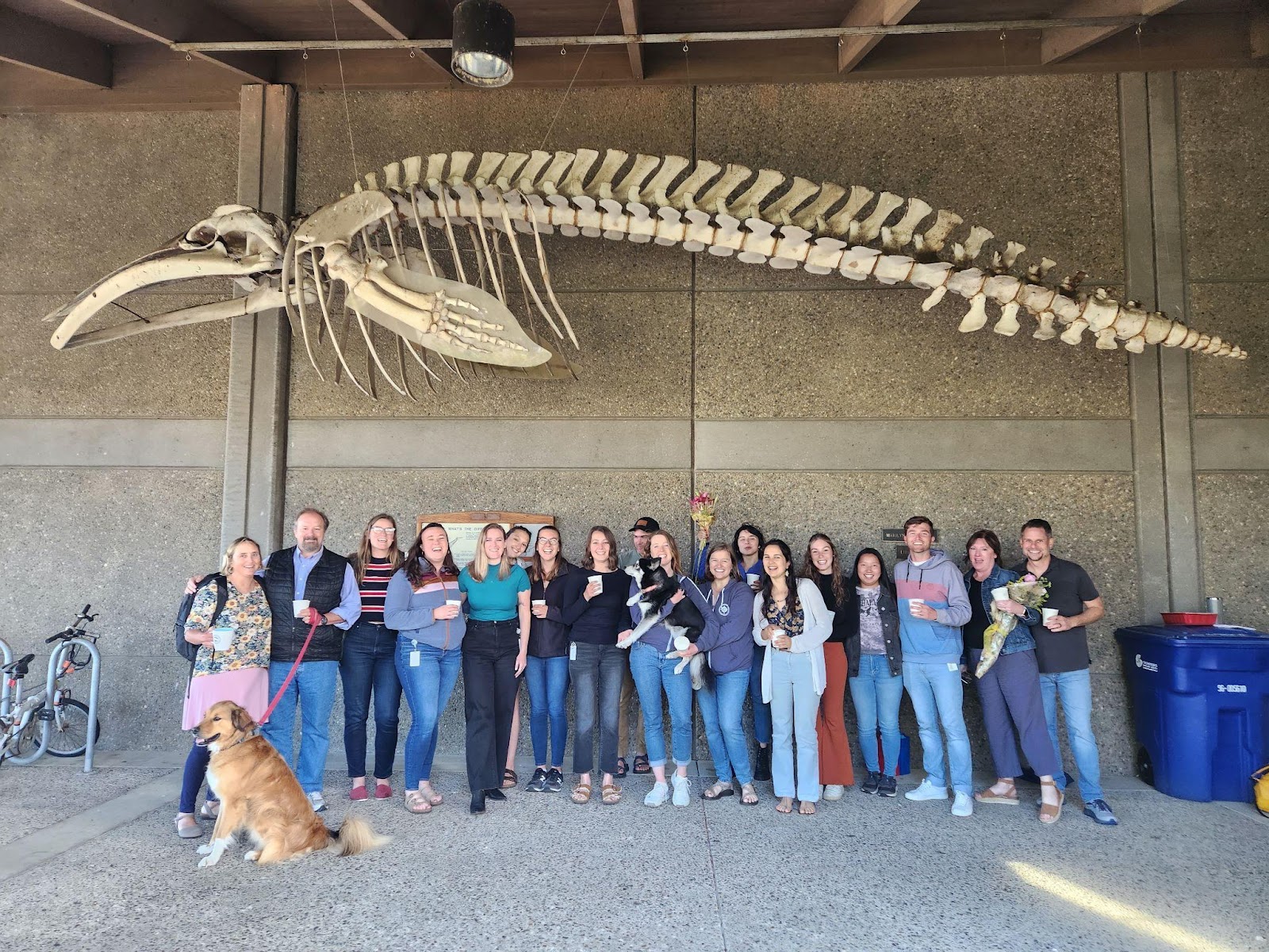
The GEMM Lab with their white elephant gifts during our annual holiday party
Did you enjoy this blog? Want to learn more about marine life, research, and conservation? Subscribe to our blog and get a weekly message when we post a new blog. Just add your name and email into the subscribe box below.
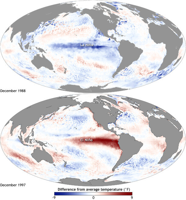
Early June marked the onset of El Niño conditions in the Pacific Ocean , which have been strengthening through the fall and winter. For Oregonians, this climate event means unseasonably warm December days, less snow and overall precipitation (it’s sunny as I write this!), and the potential for increased wildfires and marine heatwaves next summer.
This phenomenon occurs about every two to seven years as part of the El Niño Southern Oscillation (ENSO), a cyclical rotation of atmospheric and oceanic conditions in the Pacific Ocean that is initiated by departures from and returns to “normal conditions” at the equator. Typically, the trade winds blow warm water west along the equator, and El Niño occurs when these winds weaken or reverse. As a result, the upwelling of cold water at the equator ceases, and warm water flows towards the west coast of the Americas, rather than its typical pathway towards Asia. When the trade winds resume their normal direction, usually after months or a year, the system returns to “normal” conditions – or, it can enter the cool La Niña part of the cycle, in which the trade winds are stronger than normal. “El Niño de Navidad” was named by South American fisherman in the 1600s because this event tends to peak in December – and El Niño is clearly going to be a guest for Christmas this year.
Figure 1. Maps of sea surface temperature anomalies show Pacific Ocean conditions during a strong La Niña (top) and El Niño (bottom). Source: NOAA climate.gov
These events at the equator trigger changes in global atmospheric circulation patterns, and they can shape weather around the world. Teleconnection, the coherence between meteorological and environmental phenomena occurring far apart, is to me one of the most incredible things about the natural world. This coherence means that the biological community off the Oregon coast is strongly impacted by events initiated at the equator, with consequences that we don’t yet fully understand.
The effects of El Niño are diverse – floods in some places, droughts in others – and their onset can mean wildly different things for Oregon, Peru, Alaska, and beyond. As we tap our fingers waiting to be able to ski and snowboard in Oregon, what does our current El Niño event mean for the life in the waters off our coast?
Figure 2. Anomalous conditions at the equator qualified as an El Niño event in June 2023.
ENSO plays a big role in the variability in our local Northern California Current (NCC) system, and the outcomes of these events can differ based on the strength and how the signal propagates through the ocean and atmosphere (Checkley & Barth, 2009). Large-scale “coastal-trapped” waves flowing alongshore can bring the warm water signal of an El Niño to our ocean backyard in a matter of weeks. One of the first impacts is a deepening of the thermocline, the upper ocean’s steep gradient in temperature, which changes the cycling of important nutrients in the surface ocean. This can result in a decrease in upwelling and primary productivity that sends ramifications through the food web, including consequences for grazers and predators like zooplankton, marine mammals, and seabirds (Checkley & Barth, 2009).
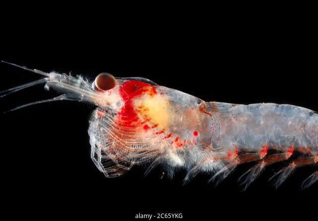
In addition to these ecosystem effects that result from local changes, the ocean community can also receive new visitors from afar, and see others flee . For krill, the shrimp-like whale prey that I spend a lot of my time thinking about, community composition can change as subtropical species typically found off southern and Baja California are displaced by horizontal ocean flow, or as resident species head north (Lilly & Ohman, 2021).
Figure 3. This Euphausia gibboides krill is typically found in offshore subtropical habitats but moves north and inshore during El Niño events, and tends to persist awhile in these new environments, impacting the local zooplankton community. Source: Solvn Zankl
The two main krill species that occur in the NCC, Euphausia pacifica and Thysanoessa spinifera, favor the cool, coastal waters typical off the coast of Oregon. During El Niño events, E. pacifica tends to contract its distribution inshore in order to continue occupying these conditions, increasing its spatial overlap with T. spinifera (Lilly & Ohman, 2021). In addition, both tend to shift their populations north, toward cooler, upwelling waters (Lilly & Ohman, 2021).
These krill species are a favored prey of rorqual whales, and the coast of Oregon is an important foraging ground for humpback, blue, and fin whales. Predators tend to follow their prey, and shifting distributions of these krill species may cause whales to move, too. During the 2014-2015 “Blob” event in the Pacific Ocean, a marine heatwave was exacerbated by El Niño conditions. Humpback whales in central California shifted their distributions inshore in response to sparse offshore krill, increasing their overlap with fishing gear and leading to an increase in entanglement events (Santora et al., 2020). Further north, these conditions even led humpback whales to forage in the Columbia River!
Figure 4. In September 2015, El Niño conditions led humpback whales to follow their prey and forage in the Columbia River.
As El Niño events compound with the impacts of global climate change, we can expect these distributional shifts – and perhaps surprises – to continue. By the year 2100, the west coast habitat of both T. spinifera and E. pacifica will likely be constrained due to ocean warming – and when El Niños occur, this habitat will decrease even further (Lilly & Ohman, 2021). As a result, the abundances of both species are expected to decrease during El Niño events, beyond what is seen today (Lilly & Ohman, 2021). This decline in prey availability will likely present a problem for future foraging whales, which may already be facing increased environmental challenges.
Understanding connections is inherent to the field of ecology, and although these environmental dependencies are part of what makes life so vulnerable, they can also be a source of resilience. Although humans have known about ENSO for over 400 years, the complex interplay between nature, anthropogenic systems, and climate change means that we are still learning the full implications of these events. Just as waiting for Santa Claus always keeps kids guessing, the dynamic ocean keeps surprising us, too.
References
Checkley, D. M., & Barth, J. A. (2009). Patterns and processes in the California Current System. Progress in Oceanography, 83(1–4), 49–64. https://doi.org/10.1016/j.pocean.2009.07.028
Lilly, L. E., & Ohman, M. D. (2021). Euphausiid spatial displacements and habitat shifts in the southern California Current System in response to El Niño variability. Progress in Oceanography, 193, 102544. https://doi.org/10.1016/j.pocean.2021.102544
Santora, J. A., Mantua, N. J., Schroeder, I. D., Field, J. C., Hazen, E. L., Bograd, S. J., Sydeman, W. J., Wells, B. K., Calambokidis, J., Saez, L., Lawson, D., & Forney, K. A. (2020). Habitat compression and ecosystem shifts as potential links between marine heatwave and record whale entanglements. Nat Commun, 11(1), 536. https://doi.org/10.1038/s41467-019-14215-w
Dr. Alejandro A. Fernández Ajó, Postdoctoral Scholar, Marine Mammal Institute – OSU Department of Fisheries, Wildlife, & Conservation Sciences, Geospatial Ecology of Marine Megafauna (GEMM) Lab.
In a previous post (link to blog), I discussed the crucial importance of acquiring knowledge on the reproductive parameters of individual animals in wild populations for designing effective strategies in conservation biology. Specifically, the ability to quantify the number of pregnancies within a population offers valuable insights into the health of individual females and the population as a whole [1,2]. This knowledge provides tools to describe important life-history parameters, including the age of sexual maturity, frequency of pregnancy, duration of gestation, timing of reproduction, and population fecundity; all of which are essential components for monitoring trends in reproduction and the overall health of a species [3]. Additionally, I explained some of the challenges inherent in obtaining such information when working with massive wild animals that spend most of their time underwater in vast expanses of the oceans. Yes, I am talking about whales.
As a result of the logistical and methodological challenges that involve the study of large whales, detailed knowledge of the life-history and general reproductive biology of whales is sparse for most species and populations. In fact, much of the available information is derived from whaling records [4], which may be outdated for application in population models [5].
If you are an avid reader of the GEMM Lab blog posts, you might be familiar with the gray whale (Eschrichtius robustus), and with the distinct subgroup of gray whales, known as the Pacific Coast Feeding Group (PCFG). PCFG gray whales are characterized by their shorter migration to spend their feeding season in the coastal waters of Northern California, Oregon, and southeastern Alaska [6], relative to the larger Eastern North Pacific gray whale that forage in the Arctic region.
The GEMM Lab has monitored individual gray whales within the PCFG off the Oregon coast since 2016 (check the GRANITE project). Each individual whale presents a unique pigmentation pattern, or unique marks that we can use to identify who is who among the whales who visit the Oregon coast. In this way, we keep a detailed record of re-sightings of known individuals (visit IndividuWhale to learn more), and we have high individual re-sighting rates, resulting in a long-term data series for individual whales which enables us to monitor their health, body condition, and thus further develop and advance our non-invasive study methods.
Drone-based image of a Gray whale defecating. Source: GEMM Lab, NOAA/NSF permit #16111
In our recently manuscript published in the Royal Society Open Science journal, armed with our robust dataset comprising fecal hormone metabolites, drone-based photogrammetry, and individual sightings, we delved into the strengths and weaknesses of various diagnostic tools for non-invasive pregnancy diagnosis. Ultimately, we propose a methodological approach that can help with the challenging and important task of identifying pregnancies in gray whales. In particular, we explored the variability in fecal progesterone metabolites and body morphology relative to observed reproductive status and estimated the pregnancy probability for mature females using statistical models.
In mammals, the progesterone hormone is secreted in the ovaries during the estrous cycle and gestation, making it the predominant hormone responsible for sustaining pregnancy [7]. As the hormones are cleared from the blood into the gut, they are metabolized and eventually excreted in feces; fecal samples represent a cumulative and integrated concentration of hormone metabolites [8;9], which are useful indicators for endocrine assessments of free-swimming whales. Additionally, our previous studies in this population [10] detected differences in body condition (see KC blog for more details about how we measure whales) that suggest that changes in the whale’s body widths could be useful in detecting pregnancies.
Our exploratory analyses show that in individual whales, the levels of fecal progesterone were elevated when pregnant as compared to when the same whale was not pregnant. But when looking at progesterone levels at the population level, these differences were masked with the intrinsic variability of this measurement. In turn, the body morphometrics, in particular the body width at the 50% of the total body length, helped discriminate pregnancies better, and the statistical models that included this width variable, effectively classified pregnant from non-pregnant females with a commendable accuracy. Thus, our morphometric approach showcased its potential as a reliable alternative for pregnancy diagnosis.
Below, a comparison of body widths at 5% increments along total body length (from 20 % to 70 %) in female gray whales of known reproductive status from UAS-based photogrammetry (example photograph shown at top). Pregnant females (PF; in blue), presumed nonpregnant juvenile females (JF; yellow), and lactating females (LF; orange). Fernandez Ajó et al. 2023.
Notably, when we ran the pregnancy prediction models on data from our 2022 season and compared results with observations of whales in 2023, we identified a known whale from our study area “Clouds” accompanied by a calf, indicating that she was pregnant in 2022. Our model predicted Clouds to be pregnant with a 70% probability. This validation lends strong confidence to our approach to diagnosing pregnancy. Conversely, some whales predicted to be pregnant in 2022 were not observed with a calf during the 2023 season. However, the absence of calves accompanying these females is likely due to the relatively high mortality of newborn calves in gray whales due to predation or other causes [11].
Overall, our findings underscore some limitations of fecal progesterone metabolite in accurately identifying pregnant PCFG gray whales. However, while acknowledging the challenges associated with fecal sample collection and hormone analysis, we advocate for ongoing exploration of alternative hormone quantification methods and antibodies. Our study highlights the importance of continued research in refining these techniques. The unique attributes of our study system, including high individual re-sighting rates and non-invasive fecal hormone analysis, position it as a cornerstone for future advancements in understanding gray whale reproductive health. By improving our ability to monitor reproductive metrics in baleen whale populations, we pave the way for more effective conservation strategies, ensuring the resilience of these magnificent creatures in the face of a changing marine ecosystems.
References
[1] Burgess EA, Lanyon JM, Brown JL, Blyde D, Keeley T. 2012 Diagnosing pregnancy in free-ranging dugongs using fecal progesterone metabolite concentrations and body morphometrics: A population application. Gen Comp Endocrinol 177, 82–92. (doi:10.1016/J.YGCEN.2012.02.008)
[2] Slade NA, Tuljapurkar S, Caswell H. 1998 Structured-Population Models in Marine, Terrestrial, and Freshwater Systems. J Wildl Manage 62. (doi:10.2307/3802363)
[3] Madliger CL, Love OP, Hultine KR, Cooke SJ. 2018 The conservation physiology toolbox: status and opportunities. Conserv Physiol 6, 1–16. (doi:10.1093/conphys/coy029)
[4] Rice DW, Wolman AA. 1971 Life history and ecology of the gray whale (Eschrichtius robustus). Stillwater, Oklahoma: American Society of Mammalogists.
[5] Melicai V, Atkinson S, Calambokidis J, Lang A, Scordino J, Mueter F. 2021 Application of endocrine biomarkers to update information on reproductive physiology in gray whale (Eschrichtius robustus). PLoS One 16. (doi:10.1371/journal.pone.0255368)
[6] Calambokidis J, Darling JD, Deecke V, Gearin P, Gosho M, Megill W, et al. Abundance, range and movements of a feeding aggregation of gray whales (Eschrichtius robustus) from California to south-eastern Alaska in 1998. J Cetacean Res Manag 2002;4:267–76.
[7] Bronson, F. H. (1989). Mammalian reproductive biology. University of Chicago Press.
[8] Wasser SK, Hunt KE, Brown JL, Cooper K, Crockett CM, Bechert U, Millspaugh JJ, Larson S, Monfort SL (2000) A generalized fecal glucocorticoid assay for use in a diverse array of nondomestic mammalian and avian species. Gen Comp Endocrinol120:260–275.
[9] Hunt, K.E., Rolland, R.M., Kraus, S.D., Wasser, S.K., 2006. Analysis of fecal glucocorticoids in the North Atlantic right whale (Eubalaena glacialis). Gen. Comp. Endocrinol. 148, 260–272. https://doi.org/10.1016/j.ygcen.2006.03.01215.
[10] Soledade Lemos L, Burnett JD, Chandler TE, Sumich JL, Torres LG. 2020 Intra‐ and inter‐annual variation in gray whale body condition on a foraging ground. Ecosphere 11. (doi:10.1002/ecs2.3094)
[11] James L. Sumich, James T. Harvey, Juvenile Mortality in Gray Whales (Eschrichtius robustus), Journal of Mammalogy, Volume 67, Issue 1, 25 February 1986, Pages 179–182, https://doi.org/10.2307/1381019
Dr. KC Bierlich, Postdoctoral Scholar, OSU Department of Fisheries, Wildlife, & Conservation Sciences, Geospatial Ecology of Marine Megafauna (GEMM) Lab
A recent blog post by GEMM Lab’s PhD Candidate Clara Bird gave a recap of our 8th consecutive GRANITEfield season this year. In her blog, Clara highlighted that we saw 71 individual gray whales this season, 61 of which we have seen in previous years and identified as belonging to the Pacific Coast Feeding Group (PCFG). With an estimated population size of around 212 individuals, this means that we saw almost 1/3 of the PCFG population this season alone. Since the GEMM Lab first started collecting data on PCFG gray whales in 2016, we have collected drone imagery on over 120 individuals, which is over half the PCFG population. This dataset provides incredible opportunity to get to know these individuals and observe them from year to year as they grow and mature through different life history stages, such as producing a calf. A question our research team has been interested in is what makes a PCFG whale different from an Eastern North Pacific (ENP) gray whale, which has a population size around 16,000 individuals and feed predominantly in the Arctic during the summer months? For this blog, I will highlight findings from our recent publication in Biology Letters (Bierlich et al., 2023) comparing the morphology (body length, skull, and fluke size) between PCFG and ENP populations.
Body size and shape reflect how an animal functions in their environment and can provide details on an individual’s current health, reproductive status, and energetic requirements. Understanding how animals grow is a key component for monitoring the health of populations and their vulnerability to climate change and other stressors in their environment. As such, collecting accurate morphological measurements of individuals is essential to model growth and infer their health. Collecting such morphological measurements of whales is challenging, as you cannot ask a whale to hold still while you prepare the tape measure, but as discussed in a previous blog, drones provide a non-invasive method to collect body size measurements of whales. Photogrammetry is a non-invasive technique used to obtain morphological measurements of animals from photographs. The GEMM Lab uses drone-based photogrammetry to obtain morphological measurements of PCFG gray whales, such as their body length, skull length (as snout-to-blowhole), and fluke span (see Figure 1).
Figure 1. Morphological measurements obtained via photogrammetry of a Pacific Coast Feeding Group (PCFG) gray whale. These measurements were used to compare to individuals from the Eastern North Pacific (ENP) population.
As mentioned in this previous blog, we use photo-identification to identify unique individual gray whales based on markings on their body. This method is helpful for linking all the data we are collecting (morphology, hormones, behavior, new scarring and skin conditions, etc.) to each individual whale. An individual’s sightings history can also be used to estimate their age, either as a ‘minimum age’ based on the date of first sighting or a ‘known age’ if the individual was seen as a calf. By combining the length measurements from drone-based photogrammetry and age estimates from photo-identification history, we can construct length-at-age growth models to examine how PCFG gray whales grow. While no study has previously examined length-at-age growth models specifically for PCFG gray whales, another study constructed growth curves for ENP gray whales using body length and age estimates obtained from whaling, strandings, and aerial photogrammetry (Agbayani et al., 2020). For our study, we utilized these datasets and compared length-at-age growth, snout-to-blowhole length, and fluke span between PCFG and ENP whales. We used Bayesian statistics to account and incorporate the various levels of uncertainty associated with data collected (i.e., measurements from whaling vs. drone, ‘minimum age’ vs. ‘known age’).
We found that while both populations grow at similar rates, PCFG gray whales reach smaller adult lengths than ENP. This difference was more extreme for females, where PCFG females were ~1 m (~3 ft) shorter than ENP females and PCFG males were ~0.5 m (1.5 ft) shorter than ENP males (Figure 2, Figure 3). We also found that ENP males and females have slightly larger skulls and flukes than PCFG male and females, respectively. Our results suggest PCFG whales are shaped differently than ENP whales (Figure 3)! These results are also interesting in light of our previous published study that found PCFG whales are skinnier than ENP whales (see this previous blog post).
Figure 2. Growth curves (von Bertalanffy–Putter) for length-at-age comparing male and female ENP and PCFG gray whales (shading represents 95% highest posterior density intervals). Points represent mean length and median age. Vertical bars represent photogrammetric uncertainty. Dashed horizontal lines represent uncertainty in age estimates.
Figure 3. Schematic highlighting the differences in body size between Pacific Coast Feeding Group (PCFG) and Eastern North Pacific (ENP) gray whales.
Our results raise some interesting questions regarding why PCFG are smaller: Is this difference in size and shape normal for this population and are they healthy? Or is this difference a sign that they are stressed, unhealthy and/or not getting enough to eat? Larger individuals are typically found at higher latitudes (this pattern is called Bergmann’s Rule), which could explain why ENP whales are larger since they feed in the Arctic. Yet many species, including fish, birds, reptiles, and mammals, have experienced reductions in body size due to changes in habitat and anthropogenic stressors (Gardner et al., 2011). The PCFG range is within closer proximity to major population centers compared to the ENP foraging grounds in the Arctic, which could plausibly cause increased stress levels, leading to decreased growth.
The smaller morphology of PCFG may also be related to the different foraging tactics they employ on different prey and habitat types than ENP whales. Animal morphology is linked to behavior and habitat (see this blogpost). ENP whales feeding in the Arctic generally forage on benthic amphipods, while PCFG whales switch between benthic, epibenthic and planktonic prey, but mostly target epibenthic mysids. Within the PCFG range, gray whales often forage in rocky kelp beds close to shore in shallow water depths (approx. 10 m) that are on average four times shallower than whales feeding in the Arctic. The prey in the PCFG range is also found to be of equal or higher caloric value than prey in the Arctic range (see this blog), which is interesting since PCFG were found to be skinnier.
It is also unclear when the PCFG formed? ENP and PCFG whales are genetically similar, but photo-identification history reveals that calves born into the PCFG usually return to forage in this PCFG range, suggesting matrilineal site fidelity that contributes to the population structure. PCFG whales were first documented off our Oregon Coast in the 1970s (Figure 4). Though, from examining old whaling records, there may have been PCFG gray whales foraging off the coasts of Northern California to British Columbia since the 1920s.
Figure 4. First reports of summer-resident gray whales along the Oregon coast, likely part of the Pacific Coast Feeding Group. Capital Journal, August 9, 1976, pg. 2.
Altogether, our finding led us to two hypotheses: 1) the PCFG range provides an ecological opportunity for smaller whales to feed on a different prey type in a shallow environment, or 2) the PCFG range is an ecological trap, where individuals gain less energy due to energetically costly feeding behaviors in complex habitat while potentially targeting lower density prey, causing them to be skinnier and have decreased growth. Key questions remain for our research team regarding potential consequences of the smaller sized PCFG whales, such as does the smaller body size equate to reduced resilience to environmental and anthropogenic stressors? Does smaller size effect fecundity and population fitness? Stay tuned as we learn more about this unique and fascinating smaller sized gray whale.
References
Agbayani, S., Fortune, S. M. E., & Trites, A. W. (2020). Growth and development of North Pacific gray whales (Eschrichtius robustus). Journal of Mammalogy, 101(3), 742–754. https://doi.org/10.1093/jmammal/gyaa028
Bierlich, K. C., Kane, A., Hildebrand, L., Bird, C. N., Fernandez Ajo, A., Stewart, J. D., Hewitt, J., Hildebrand, I., Sumich, J., & Torres, L. G. (2023). Downsized: gray whales using an alternative foraging ground have smaller morphology. Biology Letters, 19(8). https://doi.org/10.1098/rsbl.2023.0043
Gardner, J. L., Peters, A., Kearney, M. R., Joseph, L., & Heinsohn, R. (2011). Declining body size: A third universal response to warming? Trends in Ecology and Evolution, 26(6), 285–291. https://doi.org/10.1016/j.tree.2011.03.005
Allison Dawn, MSc, GEMM Lab graduate, OSU Department of Fisheries, Wildlife and Conservation Sciences, Geospatial Ecology of Marine Megafauna Lab
The second year of my master’s flew by. Gone were the days of feeling new to graduate school. While I was feeling more comfortable navigating courses, balancing time at both Corvallis and HMSC campuses, and leading recruitment and logistics for the TOPAZ/JASPER field seasons, I certainly felt intimidated by my long, yet exciting, list of research goals I planned to accomplish in order to graduate in Summer 2023. Now, I am proud to say we have come a long way from my (overly ambitious) research proposal and simple Pearson correlations.
At this time last year, I had narrowed down a few key environmental factors to assess relationships between zooplankton in reef systems where PCFG gray whales feed and environmental variability. Even still, I was feeling frustrated at my preliminary analysis results that suggested upwelling had little to no impact on zooplankton abundance or whale foraging effort. This result was dissatisfying given what we know about the upwelling and the California Current System (CCS), so I wondered if my analysis approach, upwelling metrics, or both, were limited. However, thanks to the dedicated mentorship of Leigh, and an informal chat on the water with Aaron Galloway while dive tending for CamDO deployments, I was encouraged to dig even deeper into the literature (and subsequent debates) on the role of upwelling in the nearshore. After several inspiring meetings with the lab about our latest literature deep-dive, I reconfigured my initial hypotheses and charged ahead into the next phases of analysis with a different metric of upwelling than I had calculated before, which I will describe further below.While my final chapter includes a total of seven environmental factors that capture both broad- and fine-temporal temporal scales, for the purposes of this blog I will just share the result of the broad-scale impact of intermittent upwelling on both zooplankton abundance and gray whale foraging effort.
First, a brief recap on upwelling — during the spring and summer in the CCS, strong northerly winds push surface waters offshore, bringing cold, nutrient rich waters from the deep; which creates coastal upwelling. However, upwelling is not persistent. There are periods of time when these northerly winds relax, reducing surface water advection, and upwelling stalls. This relaxation period allows for nearshore retention of primary productivity, which permeates trophic levels with important nutrients. The alternation between upwelling and relaxation is called “intermittent upwelling”, and researchers are finding that the occurrence of relaxation periods are just as important as upwelling itself. Both support biophysical mechanisms that deliver and retain nutrients in the system.
For an example of intermittent upwelling in the CCS, Figure 1 shows a northerly wind stress plot taken from a coastal buoy near our Port Orford study area during 2016. On the y-axis we have northerly wind stress, where positive values show less strong northerly winds, indicating downwelling favorable conditions, and negative values represent strong northerly winds, indicating upwelling favorable conditions. The x-axis is months over time. Here, you can see how in the winter downwelling prevails, but in the summer time we mainly have upwelling favorable winds. However, these summer periods are punctuated by positive values of wind stress, demonstrating that alternations between upwelling and relaxation occur several times throughout the spring and summer period.
Figure 1: Example plot of northerly wind stress plot taken from NOAA Buoy 4601 in 2016 (near our Port Orford, Oregon study area).
The role of upwelling intermittency has been explored in previous work and was posited as the Intermittent Upwelling Hypothesis (IUH) by Menge and Menge 2013. Figure 2, left, demonstrates this hypothesis in theoretical plots. In panel A we see that the rates of ecological processes such as primary productivity and prey response are maximal in at middle values of persistent upwelling and downwelling. In panel B. we see ecological processes positively increase with an index of upwelling intermittency. In Figure 2, right, the authors tested this hypothesis on chlorophyll-a and barnacle and mussel larval recruitment across several study sites and found the results did closely match theory.
Figure 2: Left, Intermittent Upwelling Hypothesis (IUH) theoretical plots showing predicted unimodal relationship between nutrient availability and prey response along a gradient between persistent upwelling and persistent downwelling (panel A) and the expected linear relationship between nutrient availability and upwelling intermittency (panel B); Right, Chlorophyll-a, barnacle, and mussel recruitment responses to an upwelling and intermittency index. Menge and Menge 2013.
Nearshore systems in the CCS, like the ones described in this Menge and Menge 2013 paper, are vastly understudied. And while there is a growing body of literature investigating the role of intermittent upwelling on various prey metrics (Mace & Morgan, 2006; Roegner et al 2007; Benoit-Bird et al., 2019) as well as cetacean movement (Ryan et al., 2022), to our knowledge no study has yet assessed the role of intermittent upwelling on nearshore prey availability and marine mammal occurrence.
To investigate the role of intermittent upwelling, we used the coastal upwelling transport index (CUTI) as our proxy for upwelling. Using daily CUTI values we generated a cumulative upwelling index and number of relaxation events for each year of the study (Figure 3.). This cumulative upwelling information was used to define the day of spring transition (ST) and end of the upwelling season for each year (2016-2021), following the upwelling phenological definitions from Bograd et al. 2009.
Figure 3: Summed running mean of Cumulative Upwelling Transport Index (CUTI) at latitude 42°N across years 2016-2021, initial data source https://oceanview.pfeg.noaa.gov/products/upwelling/cutibeuti
Using of five-year dataset we investigated functional relationships between each environmental variable and either zooplankton abundance or whale foraging effort using Boosted Regression Tree analysis (Elith et al., 2008). Model results demonstrate that for both zooplankton and whales, species occurrence is high at the intersection between moderate values of accumulated upwelling and with an increasing number of relaxation events. Overall, this work identifies intermittent upwelling as a primary driver of zooplankton abundance and gray whale foraging effort in a nearshore region of Oregon.
Winds in the California Current System are projected to get stronger with climate change, and if upwelling-favorable winds increase in duration and intensity, this could potentially threaten this balance between relaxation and upwelling. While these changes may mean greater primary productivity on some scales, how exactly this increase might affect the very nearshore regions and intermittent upwelling is unknown. Thus, research should continue long-term monitoring of nearshore areas to assist with adaptive management solutions in the face of environmental change.
Preparing this manuscript for my first-first author publication has been another new and exciting process. I feel so grateful for my time as a Master’s student in the GEMM Lab, and for the support of my lab mates, the HMSC community, family, and friends who cheered me on each step of the way to the finish line.
Figure 4: Toasting to a successful master’s defense seminar with GEMM Lab mates, friends and family.
Did you enjoy this blog? Want to learn more about marine life, research, and conservation? Subscribe to our blog and get a weekly message when we post a new blog. Just add your name and email into the subscribe box below.
References
Benoit‐Bird, K. J., Waluk, C. M., & Ryan, J. P. (2019). Forage species swarm in response to coastal upwelling. Geophysical Research Letters, 46(3), 1537-1546.
Bograd, S. J., Schroeder, I., Sarkar, N., Qiu, X., Sydeman, W. J., & Schwing, F. B. (2009). Phenology of coastal upwelling in the California Current. Geophysical Research Letters, 36(1).
Curtis Roegner, G., Armstrong, D. A., Hickey, B. M., & Shanks, A. L. (2003). Ocean distribution of Dungeness crab megalopae and recruitment patterns to estuaries in southern Washington State. Estuaries, 26, 1058-1070.
Elith, J., Leathwick, J. R., & Hastie, T. (2008). A working guide to boosted regression trees. Journal of animal ecology, 77(4), 802-813.
Mace, A. J., & Morgan, S. G. (2006). Biological and physical coupling in the lee of a small headland: contrasting transport mechanisms for crab larvae in an upwelling region. Marine Ecology Progress Series, 324, 185-196.
Menge, B. A., & Menge, D. N. (2013). Dynamics of coastal meta‐ecosystems: the intermittent upwelling hypothesis and a test in rocky intertidal regions. Ecological Monographs, 83(3), 283-310.
Oestreich, W. K., Abrahms, B., McKenna, M. F., Goldbogen, J. A., Crowder, L. B., & Ryan, J. P. (2022). Acoustic signature reveals blue whales tune life‐history transitions to oceanographic conditions. Functional Ecology, 36(4), 882-895.
Roegner, G. C., Armstrong, D. A., & Shanks, A. L. (2007). Wind and tidal influences on larval crab recruitment to an Oregon estuary. Marine Ecology Progress Series, 351, 177-188.
Ryan, J. P., Benoit‐Bird, K. J., Oestreich, W. K., Leary, P., Smith, K. B., Waluk, C. M., … & Goldbogen, J. A. (2022). Oceanic giants dance to atmospheric rhythms: Ephemeral wind‐driven resource tracking by blue whales. Ecology Letters, 25(11), 2435-2447.
Last month I had the privilege to participate in the 2023 September Northern California Current (NCC) cruise onboard the NOAA RV Bell M. Shimada. These cruises are part of a long-term NOAA/NWFSC effort to study the NCC ecosystem and they have been taking place every February, May, and September since 2002. Thanks to a collaboration with NOAA (and more specifically the NCC cruise chief scientist Jennifer Fisher), the GEMM Lab has been able to put marine mammal observers on these cruises since 2018.
As a postdoc working on the OPAL project, I have been the main person in charge of processing and analyzing the cetacean data collected across the 10 (now 11!) cruises that the GEMM lab participated in. These data have played a paramount role in improving our understanding of rorqual whale (e.g., blue, humpback, fin) distribution and habitat use off the coast of Oregon (Derville et al., 2022) and assessing the resulting risk of entanglement in fishing gear that they face while migrating and feeding in our waters (Derville et al., 2023). But while I have been very involved in the data analysis side of things, up to now I had never been able to contribute to data collection for this project. First, I was working remotely at the height of the COVID pandemic and second, because the NCC cruises are onboard a NOAA vessel, they have strict limitations on non-US citizens participation. So, you can imagine how excited I was (as a French citizen) to finally set foot on the famous Bell M. Shimada that I had heard so many stories about!
The NCC cruises illustrate how valuable long-term ecosystem monitoring is. Station after station, miles surveyed after miles surveyed, little by little, we learn about the complex ecological relationships and changing patterns that shape life in the ocean. The data, the experience, and the memories accumulated over the years are a true legacy that I have felt very proud to be part of. Finally, being on this ship, I felt like I was walking in the path of so many of my friends who had held those same binoculars before. Florence Sullivan, who pioneered the GEMM Lab’s NCC cruise observer effort in the harsh winter weather of February 2018. Alexa Kownacki (May 2018, May 2019), whose detailed field notes I read years later with emotion and appreciation as they helped me figure out how the Seebird software used to collect data back then (and abandoned since!). Dawn Barlow (Sep 2018, Sep 2019, Sep 2020, May 2021, May 2022), our master observer who is said to be able to detect a whale’s blow 10 miles away in a 10-foot swell and Beaufort sea state 6, all while sipping an Affogato coffee. Clara Bird (Sep 2020, May 2022), who abandoned her beloved nearshore gray whales (twice!) to sail all the way to the NH-200 station (200 nautical miles from land!). Rachel Kaplan (May 2021, May 2022, Sep 2022), our jack of all trades who concurrently studies krill and whales, and by doing so probably broke the record of numbers of times running up and down between the flying bridge and the echosounder screen room down below. Renee Albertson (Sep 2022), a Marine Mammal Institute research associate who shared observations with Rachel until the cruise was cut short by an engine issue that led them to the docks of Seattle. And finally, Craig Hayslip (May 2023), who swapped his usual observer work on the United States Coast Guard’s helicopters as part of the OPAL project for two weeks onboard the Shimada.
What a team!
From left to right and top to bottom:Florence; Alexa; Dawn; Clara; Renee, Rachel and the rest of the science team including Jennifer Fisher and Anna Bolm; Craig; Rachel; and I!
The 11th NCC cruise with GEMM Lab observers onboard was equal to its predecessors as it provided a perfect combination of camaraderie, natural beauty, Pacific Northwest weather, and unexpected change of plans. After being delayed by one day, we discovered that a big storm system was coming upon us and would have us retreat to Yaquina Bay in Newport for 4 days! Overall, I spent 5 days surveying for marine mammals from the flying bridge, in conditions that went from a beautiful sunny Friday on September 22nd to an impressive Beaufort sea state 7 on the 29th. This experience was the king of weather in which it became particularly cool to be on a ship as big as the Shimada (63 m, 208 feet long!) that can withstand swell and wind better than any ship I had worked on before.
Overall, I observed 36 groups of cetaceans, including seven different species of dolphins and whales: one sperm whale, a possible Sei whale, several fin whales, blue whales, humpback whales, and pods of Pacific white-sided dolphins, Dall’s porpoises and common dolphins. Among the highlights of this cruise was the observation of several blue whales and humpback whales that seemed to be feeding on the western slope of the Heceta bank. My personal favorite memory was also to observe common dolphins -a species that despite its name is not that common (at least not in the nearshore environment) and that I had never seen before in my life! How magnificent and graceful they were… and how lucky was I to be part of this voyage.
From left to right, top to bottom: a CTD deployment from the Bell M. Shimada; a whale’s dinner? Krill collected with a bongo net during a previous cruise; a very distant yet unmistakable sperm whale dorsal knob; a group of common dolphins; a marine mammal observer’s work tools; a blue whale surfacing at dusk.
Derville, S., Barlow, D. R., Hayslip, C. E., & Torres, L. G. (2022). Seasonal, Annual, and Decadal Distribution of Three Rorqual Whale Species Relative to Dynamic Ocean Conditions Off Oregon, USA. Frontiers in Marine Science, 9, 868566. https://doi.org/10.3389/fmars.2022.868566
Derville, S., Buell, T. V, Corbett, K. C., Hayslip, C., & Torres, L. G. (2023). Exposure of whales to entanglement risk in Dungeness crab fishing gear in Oregon, USA, reveals distinctive spatio-temporal and climatic patterns. Biological Conservation, 109989. https://doi.org/10.1016/j.biocon.2023.109989