Marine Mammals – Page 9 – Geospatial Ecology of Marine Megafauna Laboratory

You can’t build a pyramid without the base: diving into the foundations of behavioral ecology to understand cetacean foraging

By Lisa Hildebrand, MSc student, OSU Department of Fisheries & Wildlife, Marine Mammal Institute, Geospatial Ecology of Marine Megafauna Lab

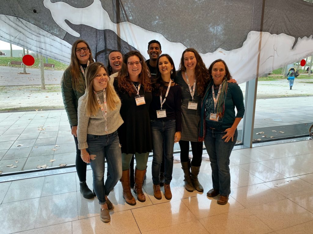
The last two months have been challenging for everyone across the world. While I have also experienced lows and disappointments during this time, I always try to see the positives and to appreciate the good things every day, even if they are small. One thing that I have been extremely grateful and excited about every week is when the clock strikes 9:58 am every Thursday. At that time, I click a Zoom link and after a few seconds of waiting, I am greeted by the smiling faces of the GEMM Lab. This spring term, our Principal Investigator Dr. Leigh Torres is teaching a reading and conference class entitled ‘Cetacean Behavioral Ecology’. Every week there are 2-3 readings (a mix of book chapters and scientific papers) focused on a particular aspect of behavioral ecology in cetaceans. During the first week we took a deep dive into the foundations of behavioral ecology (much of which is terrestrial-based) and we have now transitioned into applying the theories to more cetacean-centric literature, with a different branch of behavior and ecology addressed each week.

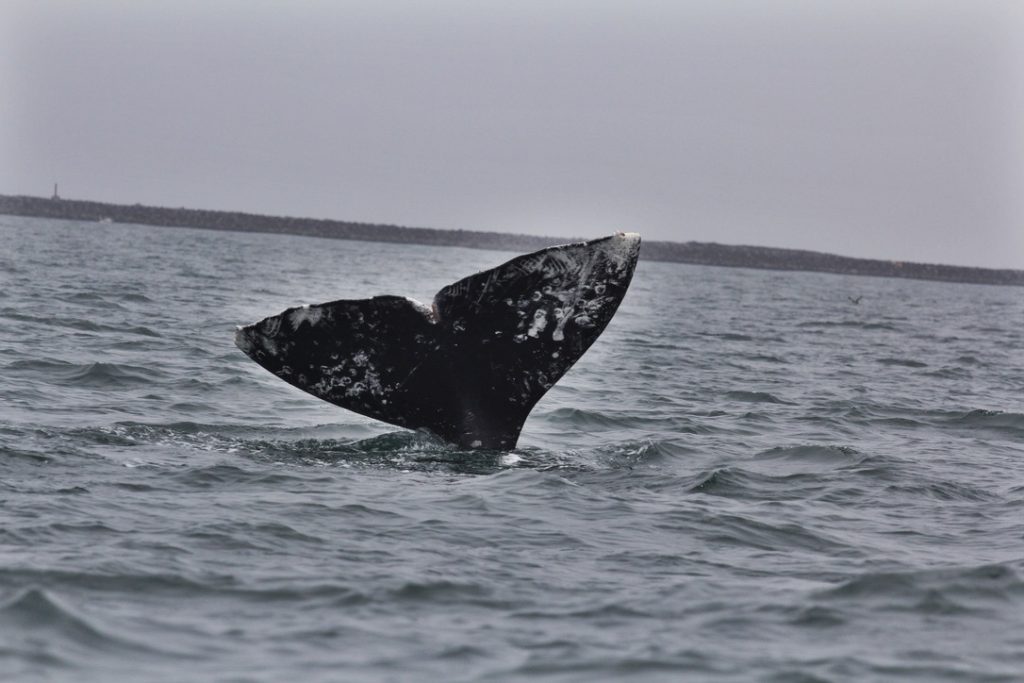
Leigh dedicated four weeks of the class to discussing foraging behavior, which is particularly relevant (and exciting) to me since my Master’s thesis focuses on the fine-scale foraging ecology of gray whales. Trying to understand the foraging behavior of cetaceans is not an easy feat since there are so many variables that influence the decisions made by an individual on where and when to forage, and what to forage on. While we can attempt to measure these variables (e.g., prey, environment, disturbance, competition, an individual’s health), it is almost impossible to quantify all of them at the same time while also tracking the behavior of the individual of interest. Time, money, and unworkable weather conditions are the typical culprits of making such work difficult. However, on top of these barriers is the added complication of scale. We still know so little about the scales at which cetaceans operate on, or, more importantly, the scales at which the aforementioned variables have an effect on and drive the behavior of cetaceans. For instance, does it matter if a predator is 10 km away, or just when it is 1 km away? Is a whale able to sense a patch of prey 100 m away, or just 10 m away? The same questions can be asked in terms of temporal scale too.

*What is that gray whale doing in the kelp? Source: F. Sullivan.*

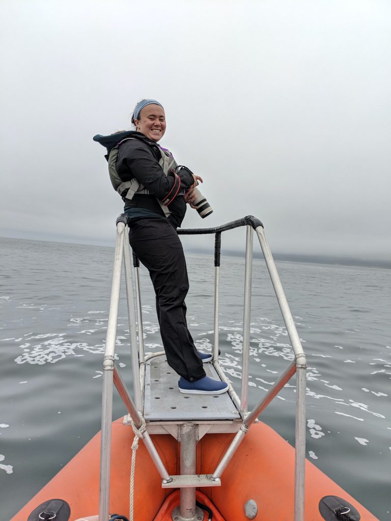
As such, cetacean field work will always involve some compromise in data collection between these factors. A project might address cetacean movements across large swaths of the ocean (e.g., the entire U.S. west coast) to locate foraging hotspots, but it would be logistically complicated to simultaneously collect data on prey distribution and abundance, disturbance and competitors across this same scale at the same time. Alternatively, a project could focus on a small, fixed area, making simultaneous measurements of multiple variables more feasible, but this means that only individuals using the study area are studied. My field work in Port Orford falls into the latter category. The project is unique in that we have high-resolution data on prey (zooplankton) and predators (gray whales), and that these datasets have high spatial and temporal overlap (collected at nearly the same time and place). However, once a whale leaves the study area, I do not know where it goes and what it does once it leaves. As I said, it is a game of compromises and trade-offs.

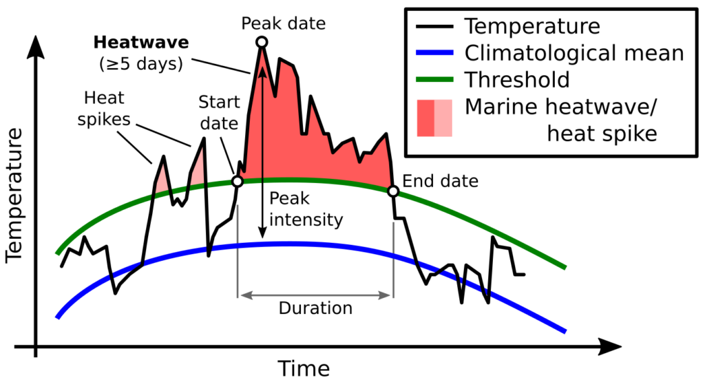
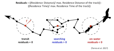
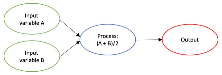
Ironically, the species and systems that we study also live a life of compromises and trade-offs. In one of this week’s readings, Mridula Srinivasan very eloquently starts her chapter entitled ‘Predator/Prey Decisions and the Ecology of Fear’ in Bernd Würsig’s ‘Ethology and Behavioral Ecology of Odontocetes’ with the following two sentences: “Animal behaviors are governed by the intrinsic need to survive and reproduce. Even when sophisticated predators and prey are involved, these tenets of behavioral ecology hold.”. Every day, animals must walk the tightrope of finding and consuming enough food to survive and ensure a level of fitness required to reproduce, while concurrently making sure that they do not fall prey to a predator themselves. Krebs & Davies (2012) very ingeniously use the idea of economic analysis of costs and benefits to understand foraging behavior (but also behavior in general). While foraging, individuals not only have to assess potential risk (Fig. 1) but also decide whether a certain prey patch or item is profitable enough to invest energy into obtaining it (Fig. 2).

Leigh’s class has been great, not only to learn about foundational theories but to then also apply them to each of our study species and systems. It has been exciting to construct hypotheses based on the readings and then dissect them as a group. As an example, Sih’s 1984 paper on the behavioral response race of predators and prey prompted a discussion on responses of predators and prey to one another and how this affects their spatial distributions. Sih posits that since predators target areas with high prey densities, and prey will therefore avoid areas that predators frequent, their responses are in conflict with one another. Resultantly, there will be different outcomes depending on whichever response dominates. If the predator’s response dominates (i.e. predators are able to seek out areas of high prey density before prey can respond), then predators and prey will have positively correlated spatial distributions. However, if the prey responses dominate, then the spatial distributions of the two should be negatively correlated, as predators will essentially always be ‘one step behind’ the prey. Movement is most often the determinant factor to describe the strength of these relationships.

Video 1. Zooplankton closest to the camera will jump or dart away from it. Source: GEMM Lab.

So, let us think about this for gray whales and their zooplankton prey. The latter are relatively immobile. Even though they dart around in the water column (I have seen them ‘jump’ away from the GoPro when we lower it from the kayak on several occasions; Video 1), they do not have the ability to maneuver away fast or far enough to evade a gray whale predator moving much faster. As such, the predator response will most likely always be the strongest since gray whales operate at a scale that is several orders of magnitude greater than the zooplankton. However, the zooplankton may not be as helpless as I have made them seem. Based on our field observations, it seems that zooplankton often aggregate beneath or around kelp. This behavior could potentially be an attempt to evade predators as the kelp and reef crevices may serve as a refuge. So, in areas with a lot of refuges, the prey response may in fact dominate the relationship between gray whales and zooplankton. This example demonstrates the importance of habitat in shaping predator-prey interactions and behavior. However, we have often observed gray whales perform “bubble blasts” in or near kelp (Video 2). We hypothesize that this behavior could be a foraging tactic to tip the see-saw of predator-prey response strength back into their favor. If this is the case, then I would imagine that gray whales must decide whether the energetic benefit of eating zooplankton hidden in kelp refuges outweighs the energy required to pursue them (Fig. 2). On top of all these choices, are the potential risks and threats of boat traffic, fishing gear, noise, and potential killer whale predation (Fig. 1). Bringing us back to the analogy of economic analysis of costs and benefits to predator-prey relationships. I never realized it so clearly before, but gray whales sure do have a lot of decisions to make in a day!

Video 2. Drone footage of a gray whale foraging in kelp and performing a “bubble blast” at 00:40. Footage captured under NMFS permit #21678. Source: GEMM Lab.

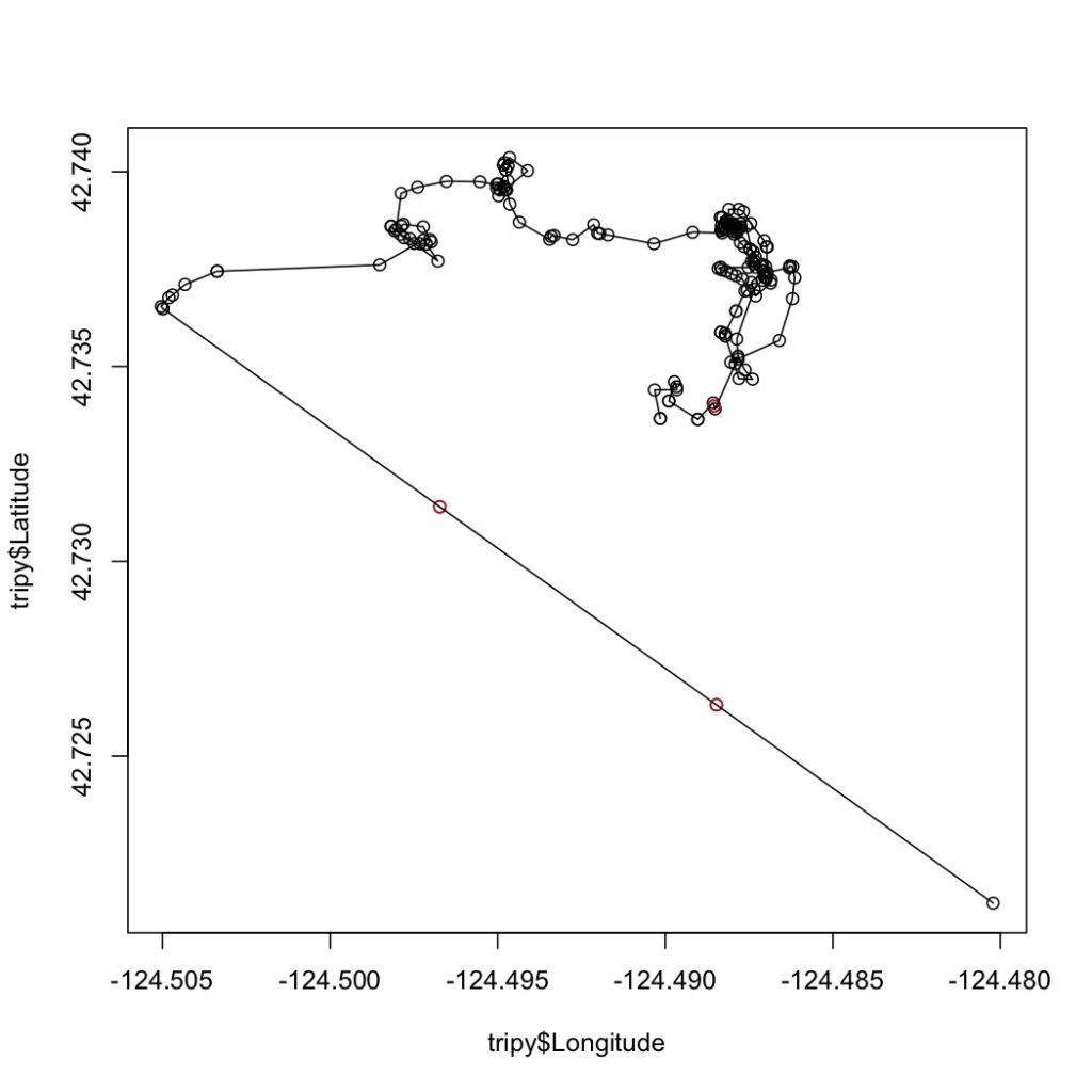
Trying to tease apart these nuanced dynamics is not easy when I am unable to simply ask my study subjects (gray whales) why they decided to abandon a patch of zooplankton (Were the zooplankton too hard to obtain because they sought refuge in kelp, or was the patch unprofitable because there were too few or the wrong kind of zooplankton?). Or, why do gray whales in Oregon risk foraging in such nearshore coastal reefs where there is high boat traffic (Does their need for food near the reefs outweigh this risk, or do they not perceive the boats as a risk?). So, instead, we must set up specific hypotheses and use these to construct a thought-out and informed study design to best answer our questions (Mann 2000). For the past few weeks, I have spent a lot of time familiarizing myself with spatial packages and functions in R to start investigating the relationships between zooplankton and kelp hidden in the data we have collected over 4 years, to ultimately relate these patterns to gray whale foraging. I still have a long and steep journey before I reach the peak but once I do, I hope to have answers to some of the questions that the Cetacean Behavioral Ecology class has inspired.

Literature cited

Krebs, J. R., and N. B. Davies. 2012. Economic decisions and the individual in Davies, N. B. et al., eds. An introduction to behavioral ecology. John Wiley & Sons, Oxford.

Mann, J. 2000. Unraveling the dynamics of social life: long-term studies and observational methods in Mann, J., ed. Cetacean societies: field studies of dolphins and whales. University of Chicago Press, Chicago.

Sih, A. 1984. The behavioral response race between predator and prey. The American Naturalist 123:143-150.

Srinivasan, M. 2019. Predator/prey decisions and the ecology of fear in Würsig, B., ed. Ethology and ecology of odontocetes. Springer Nature, Switzerland.

Can marine mammals get coronavirus?

By Lisa Hildebrand, MSc student, OSU Department of Fisheries & Wildlife, Marine Mammal Institute, Geospatial Ecology of Marine Megafauna Lab

I want to start my post this week with a disclaimer – I am not a virologist or an epidemiologist. My knowledge and understanding on what a virus is, how it changes and spreads, and predicting its trajectory, is very limited (though it has definitely improved in recent weeks). Nevertheless, I did not want that to stop me from shifting my focus and time currently spent reading about a certain virus in humans, to thinking about viruses in marine mammals. So, after several hours of reading papers and reports, I believe I have a good enough grasp on viruses in marine mammals to write a blog post on this topic.

To answer the question in my title – yes, marine mammals can get coronavirus! Coronaviruses have been detected in several marine mammals – mostly in captive ones (harbor seal, beluga whale, Indo-Pacific bottlenose dolphin), but it was also detected in a wild harbor seal¹. It is at this point where I am going to step back from marine mammals for a moment and give a very short ‘lesson’ on viruses.

Viruses are microscopic infectious agents that replicate inside living cells of organisms. They have the ability to infect all forms of life – anything from bacteria to plants to animals to humans. Nothing is excluded. Viruses are classified similarly to how living organisms are classified. Try to think back to middle school science when your teacher used mnemonic devices like, “Kids prefer candy over fancy green salad” or “Kings play chess on fine glass surfaces”, to get you to remember the Kingdom-Phylum-Class-Order-Family-Genus-Species classification. Well, viruses have almost the same classification tree. The only difference is that instead of Kingdom at the top, viruses have a Realm. As of 2019, the International Committee on Taxonomy of Viruses (ICTV) has defined 5,560 species of viruses in over 1,000 genera and 150 families. Different species of virus are classified based on their genomic material and key elements of structure and replication. That is as far as I am going to go with virus background – back to marine mammals!

*Grey seal hauled out along the west coast of the U.K. Source: L. Hildebrand.*

So, yes, coronaviruses have been detected in marine mammals before. But, no, they were not the same species of coronavirus that is currently spreading across the globe in humans. Coronavirus, or Coronaviridae, is a family of viruses that contains around 40 species. However, coronavirus is not the family that has plagued marine mammals the most since research on marine mammal diseases began. The infectious disease that I have found to be the most common and recurring in marine mammals is morbillivirus and I will therefore focus on that virus for the rest of this post.

Morbillivirus is a genus of viruses in the family Paramyxoviridae and hosts of this genus include humans, dogs, cats, cattle, seals, and cetaceans. There are seven described species of morbillivirus, three of which have been detected in marine mammals, namely canine distemper virus (CDV), cetacean morbillivirus (CeMV), and phocine distemper virus (PDV). The earliest, traceable case of morbillivirus in a marine mammal occurred in 1982 in bottlenose dolphins in the Indian and Banana Rivers in Florida². This case was followed by hundreds of others in subsequent years all along the Atlantic U.S. coast and resulted in the first Unusual Mortality Event (UME; 1987-1988) that was concluded to have been caused by morbillivirus (Table 1).

Table 1. Unusual Mortality Events (UMEs) of marine mammals in the U.S. where the cause was determined to be or is suspected to be morbillivirus. Data obtained from NOAA Fisheries.

Interestingly, at the same time as this 1980s morbillivirus in the US, the first documented marine mammal morbillivirus epidemic occurred in Europe in the North Sea. This outbreak led to the death of more than 23,000 harbor seals, which accounted for roughly 60% of all North Sea harbor seals at the time³. The virus that was isolated from the stranded seals in the North Sea was similar to CDV but not exactly the same. Resultantly, it was described as a new species of morbillivirus and it was therefore the first outbreak of PDV. Another interesting thing about this case in Europe is that while the infection originated at the Danish island of Anholt, new centers of infection appeared quite far from this first epicenter within a relatively short amount of time (~3-4 weeks) from the initial outbreak, some as far as the Irish Sea (~2,000 km away; Figure 1). Harbor seals typically have a limited home range and do not travel such distances, leading scientists to speculate that grey seals may have been a carrier of the virus and transported it from Anholt to haul-out sites in the Irish Sea. Mixed species haul-out sites of harbor and grey seals are very common across the North Sea and is the most logical explanation for the rapid spread of the virus across such distances.

*Figure 1. Map of the North Sea showing Anholt island (red marker) and the Irish Sea (white circle).*

Harbor seals seem to be the most susceptible to PDV based on all documented cases of PDV outbreaks, however the reason for this pattern remains unknown¹. While CDV has only been detected in Baikal and Caspian seals, CeMV has occurred in a larger number of cetaceans including harbor porpoises, striped, bottlenose, Guiana and Fraser’s dolphins, pilot whales, and a minke whale. This list is not extensive as morbillivirus has been found in 23 of the 90 cetacean species. In fact, it has been suggested that CeMV should be divided into more than one species as the morbilliviruses detected in the Northern Hemisphere show significant divergence from those found in the Southern Hemisphere.

Transmission is believed to mostly occur horizontally, meaning that the morbillivirus is passed from one individual to another. This transfer happens when one individual inhales the aerosolized virus breathed out by an infected individual. This is likely the reason why odontocete and pinniped groups are most affected due to their social group behavior and/or high density of individuals within groups⁴. However, vertical transmission has also been suggested as a possible transmission route as morbillivirus antigens have been detected in the mammary glands of bottlenose dolphins along the U.S. Atlantic Coast⁵ and striped dolphins in the Mediterranean Sea affected by CeMV⁶. Thus, it has been postulated that CeMV infected females could transmit the infection to their fetuses and neonates in utero, as well as to their calves during lactation.

*Bottlenose dolphins populations have been involved in several UME events related to morbillivirus along the U.S. coasts (Table 1). Source: L. Hildebrand. Image captured under NMFS permit #19116.*

Morbilliviruses mostly affect the respiratory and neurologic systems in marine mammals, wherein affected individuals may display ocular and naval discharge, erratic swimming, respiratory distress, raised body temperature, and/or cachexia (weakness and wasting away of the body due to severe illness). However, most diagnoses occur post-mortem. Some individuals may survive the initial acute infection of morbillivirus, yet the general weakening of the immune system will make individuals more susceptible to other infections, diseases, and disturbance events⁷.

It is impossible to know whether marine mammals take precautions when a virus has taken grip of a group or population, or if marine mammals even have an awareness of such things occurring. There obviously is no such thing as an emergency room or a doctor in the lives of marine mammals, but do individuals perhaps demonstrate social distancing by increasing the space between each other when traveling in groups? Do groups decrease their traveling distances or foraging ranges to isolate themselves in a smaller area? Are sick individuals ‘quarantined’ by being forced out of a group? These are just some of the questions I have been asking myself while working from home (day 16 for me now). I hope you are all staying safe and healthy and have enjoyed distracting yourselves from thinking about one virus to learn about another in a different kind of mammal.

Literature cited

¹ Bossart, G. D., and P. J. Duignan. 2018. Emerging viruses in marine mammals. CAB Reviews 13(52): doi:10.1079/PAVSNNR201913052.

² Duignan, P. J., C. House, D. K. Odell, R. S. Wells, L. J. Hansen, M. T. Walsh, D. J. St. Aubin, B. K. Rima, and J. R. Geraci. 1996. Morbillivirus infection in bottlenose dolphins: evidence for recurrent epizootics in the western Atlantic and Gulf of Mexico. Marine Mammal Science 12(4):499-515.

³ Härkönen, T., R. Dietz, P. Reijnders, J. Teilmann, K. Harding, A. Hall, S. Brasseur, U. Siebert, S. J. Goodman, P. D. Jepson, T. D. Rasmussen, and P. Thompson. 2006. A review of the 1988 and 2002 phocine distemper virus epidemics in European harbor seals. Diseases of Aquatic Organisms 68:115-130.

⁴ Van Bressem, M-F., P. J. Duignan, A. Banyard, M. Barbieri, K. M. Colegrove, S. De Guise, G. Di Guardo, A. Dobson, M. Domingo, D. Fauquier, A. Fernandez, T. Goldstein, B. Grenfell, K. R. Groch, F. Gulland, B. A. Jensen, P. D. Jepson, A. Hall, T. Kuiken, S. Mazzariol, S. E. Morris, O. Nielsen, J. A. Raga, T. K. Rowles, J. Saliki, E. Sierra, N. Stephens, B. Stone, I. Tomo, J. Wang, T. Waltzek, and J. F. X. Wellehan. 2014. Cetacean morbillivirus: current knowledge and future directions. Viruses 6(12):5145-5181.

⁵ Schulman, F. Y., T. P. Lipscomb, D. Moffett, A. E. Krafft, J. H. Lichy, M. M. Tsai, J. K. Taubenberger, and S. Kennedy. 1997. Histologic, immunohistochemical, and polymerase chain reaction studies of bottlenose dolphins from the 1987-1988 United States Atlantic coast epizootic. Veterinary Pathology 34(4):288-295.

⁶ Domingo, M., J. Visa, M. Pumarola, A. J. Marco, L. Ferrer, R. Rabanal, and S. Kennedy. 1992. Pathologic and immunocytochemical studies of morbillivirus infection in striped dolphins (Stenella coeruleoalba). Veterinary Pathology 29(1):1-10.

⁷ Wellehan, J., and G. Cortes-Hinojosa. 2019. Marine Mammal Viruses. Fowler’s Zoo and Wild Animal Medicine Current Therapy 9:597-602.

Marine heatwaves and their impact on marine mammals

By Dawn Barlow, PhD student, OSU Department of Fisheries and Wildlife, Geospatial Ecology of Marine Megafauna Lab

In recent years, anomalously warm ocean temperatures known as “marine heatwaves” have sparked considerable attention and concern around the world. Marine heatwaves (MHW) occur when seawater temperatures rise above a seasonal threshold (greater than the 90^th percentile) for five consecutive days or longer (Hobday et al. 2016; Fig. 1). With global ocean temperatures continuing to rise, we are likely to see more frequent and more intense MHW conditions in the future. Indeed, the global prevalence of MHWs is increasing, with a 34% rise in frequency, a 17% increase in duration, and a 54% increase in annual MHW days globally since 1925 (Oliver et al. 2018). With sustained anomalously warm water temperatures come a range of ecological, sociological, and economic consequences. These impacts include changes in water column structure, primary production, species composition, marine life distribution and health, and fisheries management including closures and quota changes (Oliver et al. 2018).

**Figure 1.** Illustration of how marine heatwaves are defined. Source: marineheatwaves.org

The notorious “warm blob” was an MHW event that plagued the northeast Pacific Ocean from 2014-2016. Some of the most notable consequences of this MHW were extremely high levels of domoic acid, extreme changes in the biodiversity of pelagic species, and an unprecedented delay in the opening of the Dungeness crab fishery, which is an important and lucrative fishery for the West Coast of the United States (Santora et al. 2020). The “warm blob” directly impacted the California Current ecosystem, which is typically a highly productive coastal area driven by seasonal upwelling. Yet, as a consequence of the 2014-2016 MHW, upwelling habitat was compressed and constricted to the coastal boundary, resulting in a contraction in available habitat for humpback whales and a shift in their prey (Santora et al. 2020; Fig. 2).

**Figure 2.** A figure from Santora et al. 2020 illustrating the compression in available upwelling habitat, defined by areas with SST<12°C (delineated by the black line), during the 2014-2016 marine heatwave in the California Current ecosystem.

Shifting to an example from another part of the world, the austral summer of 2015-2016 coincided with a strong regional MHW in the Tasman Sea between Australia and New Zealand, which lasted for 251 days and had a maximum intensity of 2.9°C above the climatological average (Oliver et al. 2017). Subsequently, the conditions were linked to a significant shift in zooplankton species composition and abundance in Australia (Evans et al. 2020). Ocean warming, including MHWs, also appears to decrease primary production in the Tasman Sea and large portions of New Zealand’s marine ecosystem (Chiswell & Sutton 2020). In New Zealand’s South Taranaki Bight region, where we study the ecology of blue whales, we observed a shift in blue whale distribution in the MWH conditions of February 2016 relative to more typical ocean conditions in 2014 and 2017 (Fig. 3). The first chapter of my dissertation includes a detailed analysis of the impacts of the 2016 MHW on New Zealand oceanography, krill, and blue whales, documenting how the warm, stratified water column of 2016 led to consequences across multiple trophic levels, from phytoplankton, to zooplankton, to whales.

**Figure 3.** Maps showing monthly sea surface temperature (SST) in the South Taranaki Bight region of New Zealand during our three years of survey effort to document blue whale distribution (February 2014, 2016, and 2017). Vessel tracklines are shown in black, with blue whale sighting locations shown in dark red. Red circles are scaled by the number of blue whales observed at each sighting. The color ramp of SST values is consistent across the three maps, making the dramatically warmer ocean conditions of 2016 evident.

The response of marine mammals is tightly linked to shifts in their environment and prey (Silber et al. 2017). With MHWs and changing ocean conditions, there will likely be “winners” and “losers” among marine predators including large whales. Blue whales are highly selective krill specialists (Nickels et al. 2019), whereas other species of whales, such as humpback whales, have evolved flexible feeding tactics that allow them to switch target prey species when needed (Cade et al. 2020). In California, humpback whales have been shown to switch their primary prey from krill to fish during warm years (Fossette et al. 2017, Santora et al. 2020). By contrast, blue whales shift their distribution in response to changing krill availability during warm years (Fossette et al. 2017), however this strategy comes with increased risk and energetic cost associated with searching for prey in new areas. Furthermore, in instances when a prey resource such as krill becomes increasingly scarce for a multi-year period (Santora et al. 2020), krill specialist predators such as blue whales are at a considerable disadvantage. It is also important to acknowledge that although the humpbacks in California may at first seem to have a winning strategy for adaptation by switching their food source, this tactic may come with unforeseen consequences. Their distribution overlapped substantially with Dungeness crab fishing gear during MHW conditions in the warm blob years, resulting in record numbers of entanglements that may have population-level repercussions (Santora et al. 2020).

While this is certainly not the most light-hearted blog topic, I believe it is an important one. As warming ocean temperatures contribute to the increase in frequency, intensity, and duration of extreme conditions such as MHW events, it is paramount that we understand their impacts and take informed management actions to mitigate consequences, such as lethal entanglements as a result of compressed whale habitat. But perhaps more importantly, even as we do our best to manage consequences, it is critical that we as individuals realize the role we have to play in reducing the root cause of warming oceans, by being conscious consumers and being mindful of the impact our actions have on the climate.

References

Cade DE, Carey N, Domenici P, Potvin J, Goldbogen JA (2020) Predator-informed looming stimulus experiments reveal how large filter feeding whales capture highly maneuverable forage fish. Proc Natl Acad Sci USA.

Chiswell SM, Sutton PJH (2020) Relationships between long-term ocean warming, marine heat waves and primary production in the New Zealand region. New Zeal J Mar Freshw Res.

Evans R, Lea MA, Hindell MA, Swadling KM (2020) Significant shifts in coastal zooplankton populations through the 2015/16 Tasman Sea marine heatwave. Estuar Coast Shelf Sci.

Fossette S, Abrahms B, Hazen EL, Bograd SJ, Zilliacus KM, Calambokidis J, Burrows JA, Goldbogen JA, Harvey JT, Marinovic B, Tershy B, Croll DA (2017) Resource partitioning facilitates coexistence in sympatric cetaceans in the California Current. Ecol Evol.

Hobday AJ, Alexander L V., Perkins SE, Smale DA, Straub SC, Oliver ECJ, Benthuysen JA, Burrows MT, Donat MG, Feng M, Holbrook NJ, Moore PJ, Scannell HA, Sen Gupta A, Wernberg T (2016) A hierarchical approach to defining marine heatwaves. Prog Oceanogr.

Nickels CF, Sala LM, Ohman MD (2019) The euphausiid prey field for blue whales around a steep bathymetric feature in the southern California current system. Limnol Oceanogr.

Oliver ECJ, Benthuysen JA, Bindoff NL, Hobday AJ, Holbrook NJ, Mundy CN, Perkins-Kirkpatrick SE (2017) The unprecedented 2015/16 Tasman Sea marine heatwave. Nat Commun.

Oliver ECJ, Donat MG, Burrows MT, Moore PJ, Smale DA, Alexander L V., Benthuysen JA, Feng M, Sen Gupta A, Hobday AJ, Holbrook NJ, Perkins-Kirkpatrick SE, Scannell HA, Straub SC, Wernberg T (2018) Longer and more frequent marine heatwaves over the past century. Nat Commun.

Santora JA, Mantua NJ, Schroeder ID, Field JC, Hazen EL, Bograd SJ, Sydeman WJ, Wells BK, Calambokidis J, Saez L, Lawson D, Forney KA (2020) Habitat compression and ecosystem shifts as potential links between marine heatwave and record whale entanglements. Nat Commun.

Silber GK, Lettrich MD, Thomas PO, Baker JD, Baumgartner M, Becker EA, Boveng P, Dick DM, Fiechter J, Forcada J, Forney KA, Griffis RB, Hare JA, Hobday AJ, Howell D, Laidre KL, Mantua N, Quakenbush L, Santora JA, Stafford KM, Spencer P, Stock C, Sydeman W, Van Houtan K, Waples RS (2017) Projecting marine mammal distribution in a changing climate. Front Mar Sci.

Makah Gray Whale Hunt Waiver – a long-time coming, but still premature?

By Lisa Hildebrand, MSc student, OSU Department of Fisheries & Wildlife, Marine Mammal Institute, Geospatial Ecology of Marine Megafauna Lab

Archaeological site of Ozette Village. Source: Makah Museum.

The Makah, an indigenous people of the Pacific Northwest Coast living in Washington State, have a long history with whaling. Deposits from a mudslide in the village of Ozette suggest that whaling may date back 2,000 years as archaeologists uncovered humpback and gray whale bones and barbs from harpoons (Kirk 1986). However, the history of Makah whaling is also quite recent. On January 29 of this year, the National Marine Fisheries Service (NMFS; informally known as NOAA Fisheries) announced a 45-day public comment period regarding a NMFS proposed waiver on the Marine Mammal Protection Act’s (MMPA) moratorium on the take of marine mammals to allow the Makah to take a limited number of eastern North Pacific gray whales (ENP). To understand how the process reached this point, we first must go back to 1855.

1855 marks the year in which the U.S. government and the Makah entered into the Treaty of Neah Bay (in Washington state). The Makah ceded thousands of acres of land to the U.S. government, and in return reserved their right to whale. Following the treaty, the Makah hunt of gray whales continued until the 1920s. At this point, commercial hunting had greatly reduced the ENP population, so much so that the Makah voluntarily ceased their whaling. The next seven decades brought about the formation of the International Whaling Commission (IWC), the enactment of the Whaling Convention Act, the listing of gray whales as endangered under the U.S. Endangered Species Act, and the enactment of the MMPA. For gray whales, these national and international measures were hugely successful, leading to the removal of the ENP from the Federal List of Endangered Wildlife in 1994 when it was determined that the population had recovered to near its estimated original population size.

One year later on May 5, 1995 (just one month after I was born!), the Makah asked the U.S. Department of Commerce to represent its interest to obtain a quota for gray whales from the IWC in order to resume their treaty right for ceremonial and subsistence harvest of the ENP. The U.S. government pursued this request at the next IWC meeting, and subsequently NMFS issued a final Environmental Assessment that found no significant impact to the ENP population if the hunt recommenced. The IWC set a catch limit and NMFS granted the Makah a quota in 1998. In 1999 the Makah hunted, struck and landed an ENP gray whale.

*“Makahs cutting up whale, Neah Bay, ca. 1930. Photo by Asahel Curtis, Courtesy UW Special Collections (CUR767)”*. Source and caption: History Link.

I will not go into detail about what happened between 1999 and now because frankly, a lot happened, particularly a lot of legal events including summary judgements, appeals, and a lot of other legal jargon that I do not quite understand. If you want to know the specifics of what happened in those two decades, I suggest you look at NMFS’ chronology of the Makah Tribal Whale Hunt. In short, cases brought against NMFS argued that they did not take a “hard [enough] look” at the National Environmental Policy Act when deciding that the Makah could resume the hunt. Consequently, the hunt was put on hold. Yet, in 2005 NMFS received a waiver request from the Makah on the MMPA’s take moratorium and NMFS published a notice of intent to review this request. A lot more happened between that event and now, including on January 29 of this year when NMFS announced the availability of transcripts from the Administrative Law Judge’s (ALJ) hearing (which happened from November 14-21, 2019) on the proposed regulations and waiver to allow the Makah to resume hunting the ENP. We are currently in the middle of the aforementioned 45-day public comment period on the formal rulemaking record.

It has been 15 years since the Makah requested the waiver and while the decision has not yet been reached, we are likely nearing the end of this long process. This blog has turned into somewhat of a history lesson (not really my intention) but I feel it is important to understand the lengthy and complex history associated with the decision that is probably going to happen sometime this year. My actual intent for this blog is to ruminate on a few questions, some of which remain unanswered in my opinion, that are large and broad, and important to consider. Some of these questions point out gaps in our ecological knowledge regarding gray whales that I believe should be addressed for a truly informed decision to be made on NMFS’ proposed waiver now or anytime in the near future.

1. Should the Pacific Coast Feeding Group (PCFG) of gray whales be recognized as its own stock?

Currently, the PCFG are considered a part of the ENP stock. This decision was published following a workshop held by a NMFS task force (Weller et al. 2013). The report concluded that based on photo-identification, genetics, tagging, and other data, there was a substantial level of uncertainty in the strength of the evidence to support the independence of the PCFG from the ENP. Nevertheless, mitochondrial genetic data have indicated a differentiation between the PCFG and the ENP, and the exchange rate between the two groups may be small enough for the two to be considered demographically independent (Frasier et al. 2011). Based on all currently available data, it seems that matrilineal fidelity plays a role in creating population structure within and between the PCFG and the ENP, however there has not been any evidence to suggest that whales from one feeding area (i.e. the PCFG range) are reproductively isolated from whales that utilize other feeding areas (i.e. the Arctic ENP feeding grounds) (Lang et al. 2011). Several PCFG researchers do argue that there needs to be recognition of the PCFG as an independent stock. It is clear that more research, especially efforts to link genetic and photo-identification data within and between groups, is required.

ENP gray whales foraging off the coast of Alaska on their main foraging grounds in the Bering Sea. Photo taken by ASAMM/AFSC. Funded by BOEM IAA No. M11PG00033. Source: NMFS.

2. Is emigration/immigration driving PCFG population growth, or is it births/deaths?

It is unclear whether the current PCFG population growth is a consequence of births and deaths that occur within the group (internal dynamics) or whether it is due to immigration and emigration (external dynamics). Likely, it is a combination of the two, however which of the two has more of an effect or is more prevalent? This question is important to answer because if population growth is driven more by external dynamics, then potential losses to the PCFG population due to the Makah hunt may not be as detrimental to the group as a whole. However, if internal dynamics play a bigger role, then the loss of just a few females could have long-term ramifications for the PCFG (Schubert 2019). NMFS has taken precautions to try and avoid such effects. In their proposed waiver, of the cumulative limit of 16 strikes of PCFG whales over the 10-year waiver period, no more than 8 of the strikes may be PCFG females (Yates 2019a). While a great step, it still begs the question how the loss of 8 females, admittedly over a rather long period of time, may affect population dynamics since we do not know what ultimately drives recruitment. Especially when taken together with potential non-lethal effects on whales (further discussed in question 5 below).

“Scarlet” is a PCFG female who has had multiple calves in the decades that researchers have seen her in the PCFG range. Image captured under NOAA/NMFS permit #21678. Source: L Hildebrand.

3. How important are individual patterns within the PCFG, and how might the loss of these individuals affect the population?

The hunt will be restricted to the Makah Usual & Accustomed fishing area (U&A), which is off the Washington coast. It has been shown that site fidelity among PCFG individuals is strong. In fact, based on the 143 PCFG gray whales observed in nine or more years from 1996 to 2015, 94.4% were seen in at least one of nine different PCFG regions during six or more of the years they were seen (Calambokidis et al. 2017). While high site-fidelity seems to be common for some PCFG individuals in certain regions, interestingly, an analysis of sighting histories of all individuals that utilized the Makah U&A from 1985-2011 revealed that most PCFG whales do not have strong site fidelity to the Makah U&A (Scordino et al. 2017). Only about 20% of the whales were observed in six or more years of the total 26 years of data analyzed. Since high individual site fidelity does not appear to be strong in this area, perhaps a loss of genetic diversity, cultural knowledge, and behavioral individualism is not of great concern.

“Buttons” seems to have a preference for the southern Oregon coast as in the last 5 years the GEMM Lab has conducted research, he has only been sighted in 1 year in Newport but in all 5 years in Port Orford. However, perhaps such preferences are not common among all PCFG whales. Source: F. Sullivan.

4. How has the current UME affected the situation?

The ENP has experienced two Unusual Mortality Events (UMEs) in the past 20 years; one from 1999-2000 and the second began in May 2019. Many questions arise when thinking about the Makah hunt in light of the UME.

What impacts will the current UME have on ENP and PCFG birth rates in subsequent years?
Could the UME lead to shifts in feeding behavior of ENP whales and result in greater use of PCFG range by more individuals?
What caused the UME? Shifting prey availability and a changing climate? Or has the ENP reached carrying capacity?
Will UMEs become more frequent in the future with continued warming of the Arctic?
What is the added impact of such periodic UMEs on population trends?

*“A gray whale found dead off Point Reyes National Seashore in northern California [during the 2019 UME]. Photo by M. Flannery, California Academy of Sciences.*” Source and caption: NMFS.

A key assumption of the model developed by NMFS (Moore 2019) to forecast PCFG population size for the period 2016-2028, is that the population processes underlying the data from 2002-2015 (population size estimates developed by Calambokidis et al. 2017) will be the same during the forecasted period. In other words, it is assuming that PCFG gray whales will experience similar environmental conditions (with similar variation) during the next decade as the previous one, and that there will be no catastrophic events that could drastically affect population dynamics. The UME that is still ongoing could arguably affect population dynamics enough such that they are drastically different to effects on the population dynamics during the previous decade. The cause of the 1999/2000 UME remains undetermined and the results of the investigation of the current UME will possibly not be available for several years (Yates 2019b). Even though the ENP did rebound following the 1999/2000 UME and the abundance of the PCFG increased during and subsequent to that UME, much has changed in the 20 years since then. Increased noise due to increased vessel traffic and other anthropogenic activities (seismic surveys, pile driving, construction to name a few) as well as increased coastal recreational and commercial fishing, have all contributed to a very different oceanscape than the ENP and PCFG encountered 20 years ago. Furthermore, the climate has changed considerably since then too, which likely has caused changes in the spatial distribution of habitat and quantity, quality, and predictability of prey. All of these factors make it difficult to predict what impact the UME will have now. If such events were to become more frequent in the future or the impacts of such events are greater than anticipated, then the PCFG population forecasts will not have accounted for this change.

5. What impacts will the hunt and associated training exercises have on energy and stress levels of whales?

The proposed waiver would allow hunts to occur in the following manner: in even-years, the hunting period is from December 1 of an odd-numbered year through May 31 of the following even-numbered year. While in odd-years, the hunt is limited from July to October.

In the even-years, the hunt coincides with the northbound migration toward the foraging grounds for ENP whales and with the arrival of PCFG whales to their foraging grounds near the Makah U&A. During the northbound migration, gray whales are at their most nutritionally stressed state as they have been fasting for several months. They are therefore most vulnerable to energy losses due to disturbance at this point (Villegas-Amtmann 2019). Attempted strikes and training exercises would certainly cause some level of disturbance and stress to the whales. Furthermore, the timing of even-year hunts, means that hunters would likely encounter pregnant females, as they are the first to arrive at foraging grounds. A loss of just ~4% of a pregnant female’s energy budget could cause them to abort the fetus or not produce a calf that year (Villegas-Amtmann 2019).

In odd-years, the Makah hunt will most certainly target PCFG whales as the Makah U&A forms one of the nine PCFG regions where PCFG individuals will be feeding during those months. However, NMFS’ waiver limits the number of strikes during odd-years to 2 (Yates 2019a), which certainly protects the PCFG population.

Stress is a difficult response to quantify in baleen whales and research on stress through hormone analysis is still relatively novel. It is unlikely that a single boat training approach of a gray whale will have an adverse effect on the individual. However, a whale is never just experiencing one disturbance at a time. There are typically many confounding factors that influence a whale’s state. In an ideal world, we would know what all of these factors are and how to recognize these effects. Yet, this is virtually impossible. Therefore, while precautions will be taken to try to minimize harm and stress to the gray whales, there may very well still be unanticipated impacts that we cannot anticipate.

Gray whale fluke. Image captured under NOAA/NMFS permit #21678. Photo: L Hildebrand.

Final thoughts

Many unknowns still remain about the ENP and PCFG gray whale populations. During the ALJ hearing, both sides tried to deal with these unknowns. After reading testimony from both sides, it is clear to me that some of the unknowns still have not been reconciled. Ultimately, a lot of the questions circle back to the first one I posed above: Are the PCFG an independent stock? If there is independent population structure, then the proposed waiver put forth by NMFS would likely change. While NMFS has certainly taken the PCFG into account during the declarations of several experts at the ALJ hearing and has aired on the side of caution, the fact that the PCFG is considered part of the ENP might underestimate the impact that a resumption of the Makah hunt may have on the PCFG. As you can see, there are still many questions that should be addressed to make fully informed decisions on such an important ruling. While this research may take several years to obtain results, the data are within reach through synthesis and collaboration that will fill these critical knowledge gaps.

Literature cited

Calambokidis, J. C., J. Laake, and A. Pérez. 2017. Updated analysis of abundance and population structure of seasonal gray whales in the Pacific Northwest, 1996-2015. International Whaling Commission SC/A17/GW/05.

Frasier, T. R., S. M. Koroscil, B. N. White, and J. D. Darling. 2011. Assessment of population substructure in relation to summer feeding ground use in eastern North Pacific gray whale. Endangered Species Research 14:39-48.

Kirk, Ruth. 1986. Tradition and change on the Northwest Coast: the Makah, Nuu-chah-nulth, southern Kwakiutl and Nuxalk. University of Washington Press, Seattle.

Lang, A. R., D. W. Weller, R. LeDuc, A. M. Burdin, V. L. Pease, D. Litovka, V. Burkanov, and R. L. Brownell, Jr. 2011. Genetic analysis of stock structure and movements of gray whales in the eastern and western North Pacific. SC/63/BRG10.

Moore, J. E. 2019. Declaration in re: ‘Proposed Waiver and Regulations Governing the Taking of Eastern North Pacific Gray Whales by the Makah Indian Tribe’. Administrative Law Judge, Hon. George J. Jordan. Docket No. 19-NMFS-0001. RINs: 0648-BI58; 0648-XG584.

Schubert, D. J. 2019. Rebuttal testimony in re: ‘Proposed Waiver and Regulations Governing the Taking of Eastern North Pacific Gray Whales by the Makah Indian Tribe’. Administrative Law Judge, Hon. George J. Jordan. Docket No. 19-NMFS-0001. RINs: 0648-BI58; 0648-XG584.

Scordino, J. J., M. Gosho, P. J. Gearin, A. Akmajian, J. Calambokidis, and N. Wright. 2017. Individual gray whale use of coastal waters off northwest Washington during the feeding season 1984-2011: Implications for management. Journal of Cetacean Research and Management 16:57-69.

Villegas-Amtmann, S. 2019. Declaration in re: ‘Proposed Waiver and Regulations Governing the Taking of Eastern North Pacific Gray Whales by the Makah Indian Tribe’. Administrative Law Judge, Hon. George J. Jordan. Docket No. 19-NMFS-0001.

Weller, D. W., S. Bettridge, R. L. Brownell, Jr., J. L. Laake, J. E. Moore, P. E. Rosel, B. L. Taylor, and P. R. Wade. 2013. Report of the National Marine Fisheries Service Gray Whale Stock Identification Workshop. NOAA-TM-NMFS-SWFSC-507.

Yates, C. 2019a. Declaration in re: ‘Proposed Waiver and Regulations Governing the Taking of Eastern North Pacific Gray Whales by the Makah Indian Tribe’. Administrative Law Judge, Hon. George J. Jordan. Docket No. 19-NMFS-0001. RINs: 0648-BI58; 0648-XG584.

Yates, C. 2019b. Fifth declaration in re: ‘Proposed Waiver and Regulations Governing the Taking of Eastern North Pacific Gray Whales by the Makah Indian Tribe’. Administrative Law Judge, Hon. George J. Jordan. Docket No. 19-NMFS-0001. RINs: 0648-BI58; 0648-XG584.

Toxins in Marine Mammals: a Story

By: Alexa Kownacki, Ph.D. Student, OSU Department of Fisheries and Wildlife, Geospatial Ecology of Marine Megafauna Lab

As technology has developed over the past ten years, toxins in marine mammals have become an emerging issue. Environmental toxins are anything that can pose a risk to the health of plants or animals at a dosage. They can be natural or synthetic with varying levels of toxicity based on the organism and its physiology. Most prior research on the impacts toxins before the 2000s was conducted on land or in streams because of human proximity to these environments. However. with advancements in sampling methods, increasing precision in laboratory testing, and additional focus from researchers, marine mammals are being assessed for toxin loads more regularly.

A dolphin swims through a diesel slick caused by a small oil spill in a port. (Image Source: The Ocean Update Blog)

Marine mammals live most of their lives in the ocean or other aquatic systems, which requires additional insulation for protection from both cold temperatures and water exposure. This added insulation can take the form of lipid rich blubber, or fur and hair. Many organic toxins are lipid soluble and therefore are more readily found and stored in fatty tissues. When an organic toxin like a polychlorinated biphenyl (PCB) is released into the environment from an old electrical transformer, it persists in sediments. As these sediments travel down rivers and into the ocean, these toxic substances slowly degrade in the environment and are lipophilic (attracted to fat). Small marine critters eat the sediment with small quantities of toxins, then larger critters eat those small critters and ingest larger quantities of toxins. This process is called biomagnification. By the time a dolphin consumes large contaminated fishes, the chemical levels may have reached a toxic level.

The process by which PCBs accumulate in marine mammals from small particles up to high concentrations in lipid layers. (Image Source: World Ocean Review)

Marine mammal scientists are teaming with biochemists and ecotoxicologists to better understand which toxins are more lethal and have more severe long-term effects on marine mammals, such as decreased reproduction rates, lowered immune systems, and neurocognitive delays. Studies have already shown that higher contaminant loads in dolphins cause all three of these negative effects (Trego et al. 2019). As a component of my thesis work on bottlenose dolphins I will be measuring contaminant levels of different toxins in blubber. Unfortunately, this research is costly and time-consuming. Many studies regarding the effects of toxins on marine mammals are funded through the US government, and this is where the public can have a voice in scientific research.

Rachel Carson examines a specimen from a stream collection site in the 1950s. (Image Source: Alfred Eisenstaedt/ The LIFE picture collection/ Getty Images.)

Prior to the 1960s, there were no laws regarding the discharge of toxic substances into our environment. When Rachel Carson published “Silent Spring” and catalogued the effects of pesticides on birds, the American public began to understand the importance of environmental regulation. Once World War II was over and people did not worry about imminent death due to wartime activities, a large portion of American society focused on what they were seeing in their towns: discharges from chemical plants, effluents from paper mills, taconite mines in the Great Lakes, and many more.

Discharge from a metallic sulfide mine collects in streams in northern Wisconsin. (Image Source: Sierra Club)

However, it was a very different book regarding pollutants in the environment that caught my attention – and that of a different generation and part of society – even more than “Silent Spring”. A book called “The Lorax”. In this 1972 children’s illustrated book by Dr. Seuss, a character called the Lorax “speaks for the trees”. The Lorax touches upon critical environmental issues such as water pollution, air pollution, terrestrial contamination, habitat loss, and ends with the poignant message, “Unless someone like you cared a whole awful lot, nothing is going to get better. It’s not.”

The original book cover for “The Lorax” by Dr. Seuss. (Image source: Amazon.com)

Within a decade, the US Environmental Protection Agency (EPA) was formed and multiple acts of congress were put in place, such as the National Environmental Policy Act, Clean Air Act, Clean Water Act, and Toxic Substances Control Act, with a mission to “protect human health and the environment.” The public had successfully prioritized protecting the environment and the government responded. Before this, rivers would catch fire from oil slicks, children would be banned from entering the water in fear of death, and fish would die by the thousands. The resulting legislation cleaned up our air, rivers, and lakes so that people could swim, fish, and live without fear of toxic substance exposures.

The Cuyahoga River on fire in June 1969 after oil slicked debris ignited. (Image Source: Ohio Central History).

Fast forward to 2018 and times have changed yet again due to fear. According to a Pew Research poll, terrorism is the number one issue that US citizens prioritize, and Congress and the President should address. The environment was listed as the seventh highest priority, below Medicare (“Majorities Favor Increased Spending for Education, Veterans, Infrastructure, Other Govt. Programs.”). With this societal shift in priorities, research on toxins in marine mammals may no longer grace the covers of the National Geographic, Science, or Nature, not for lack of importance, but because of the allocation of taxpayer funds and political agendas. Meanwhile, long-lived marine mammals will still be accumulating toxins in their blubber layers and we, the people, will need to care a whole lot, to save the animals, the plants, and ultimately, our planet.

The Lorax telling the reader how to save the planet. (Image Source: “The Lorax” by Dr. Seuss via the Plastic Bank)

Citations:

“Majorities Favor Increased Spending for Education, Veterans, Infrastructure, Other Govt. Programs.” Pew Research Center for the People and the Press, Pew Research Center, 11 Apr. 2019, www.people-press.org/2019/04/11/little-public-support-for-reductions-in-federal-spending/pp_2019-04-11_federal-spending_0-01-2/.

Marisa L. Trego, Eunha Hoh, Andrew Whitehead, Nicholas M. Kellar, Morgane Lauf, Dana O. Datuin, and Rebecca L. Lewison. Environmental Science & Technology 2019 53 (7), 3811-3822. DOI: 10.1021/acs.est.8b06487

GEMM Lab 2019: A Year in the Life

By Lisa Hildebrand, MSc student, OSU Department of Fisheries & Wildlife, Geospatial Ecology of Marine Megafauna Lab

Another year has come and gone, and with the final days of 2019 upon us, it is fulfilling to look back and summarize all of the achievements in the GEMM Lab this year. So, snuggle up with your favorite holiday drink and enjoy our recap of 2019!

We wrapped up two intense but rewarding gray whale field seasons this summer. Our project investigating the health of Pacific Coast Feeding Group (PCFG) gray whales through fecal hormone and body condition sampling in the context of ocean noise went into its fourth year, while the Port Orford project where we track whales and prey at a very fine-scale celebrated its wood anniversary (five years!). The dedication and hard work of lots of people to help us collect our data meant that we were able to add a considerable amount of samples to our growing gray whale datasets. Our trusty red RHIB Ruby zipped around the Pacific and enabled us to collect 58 fecal samples, fly the drone 102 times, undertake 105 GoPro drops and record 141 gray whale sightings. Our Newport crew was a mix of full-time GEMMers (Leigh, Todd, Dawn, Leila, Clara, and myself) as well as part-time summer GEMMers (Ale, Sharon, and Cassy). Further south in Port Orford, my team of undergraduate and high school students and I had an interesting field season. We only encountered four different individuals (Buttons, Glacier, Smudge, and Primavera), however saw them repeatedly throughout the month of August, resulting in as many as 15 tracklines for one individual. Furthermore, we collected 249 GoPro drops and 248 zooplankton net samples.

Leila taking photos of gray whales from Ruby’s bow pulpit. Photo: Leigh Torres

The GEMM Lab’s fieldwork was not just restricted to gray whales. After last year’s successes aboard the NOAA ship Bell M. Shimada, Alexa and Dawn both boarded the ship again this year as marine mammal observers for the May and September cruises, respectively. They spied humpback, blue, sperm, and fin whales, as well as many dolphins and seabirds, adding to the GEMM Lab’s growing database of megafauna distribution off the Oregon coast.

Alexa observing on the R/V Shimada in May 2019, all bundled up. Image Photo: Alexa Kownacki

After winning the prestigious L’Oréal-UNESCO For Women in Science fellowship and the inaugural Louis Herman Scholarship, GEMM Lab grad Solène Derville lead her first research cruise aboard the French R/V Alis. She and her team conducted line transect surveys and micronekton/oceanographic sampling over several seamounts to try to solve the mystery of why humpbacks hang out there. We are also very excited to announce that Solène will be returning to the GEMM Lab as a post-doc in 2020! She will be creating distribution models of whales off the coast of Oregon with the data collected by Leigh during helicopter flights with the US Coast Guard. The primary aim of this work is to identify potential whale hotspots in an effort to avoid spatial overlap with fisheries gear and reduce entanglement risk.

Solène soaking wet after spending several hours observing cetaceans and seabirds on R/V Alis. Photo: Jérôme Jambou

Switching the focus from marine mammals to seabirds, Rachael has had an extremely busy year of field work all across the globe. She island-hopped from Midway (Hawaiian Northwest island) to the Falkland Islands in the first half of the year, and is currently overwintering on South Georgia, where she will be until end of February. Rachael is tracking albatross at all three locations by tagging individual birds to understand movements relative to fishing vessels and flight energetics.

Besides several field efforts, the GEMM Lab was also busy disseminating our research and findings to various audiences. Our conferences kicked off in late February when Leigh and Rachael both flew to Kauai to present at the Pacific Seabird Group’s 46^th Annual Meeting. In the spring, Leila, Dawn, Alexa, Dom, and myself drove to Seattle where the University of Washington hosted the Northwest Student Society of Marine Mammalogy chapter meeting and we all gave talks. Additionally, the Fisheries & Wildlife grad students in the lab also presented at the department’s annual Research Advances in Fisheries, Wildlife, and Ecology conference. Later in the year, Dom and I attended the State of the Coast conference where Dom was invited to participate in a panel about the holistic approaches to management in the nearshore while I presented a poster on preliminary findings of my Master’s thesis. Most recently, the entire GEMM Lab (bar Rachael) flew to Barcelona to present at the World Marine Mammal Conference (WMMC).

GEMM Lab at the WMMC. Photo: Karen Lohman

Our science communication and outreach efforts were not just restricted to conferences though. Over the course of this year, the GEMM Lab supervised a total of 10 undergraduate and high school interns that assisted in a variety of ways (field and/or lab work, data analyses, independent projects) on a number of projects going on in the lab. Leigh and Dawn boarded the R/V Oceanus in the fall to co-lead a STEM research cruise aimed at providing high school students and teachers hands-on marine research. Dawn and I were guests on Inspiration Dissemination, a live radio show run by graduate students about graduate research going on at OSU. Our weekly blog, now in its fifth year, reached its highest viewership with a total of 14,814 views this year!

The GEMMers were once again prolific writers too! The 13 new publications in 10 scientific journals include contributions from Leigh (7), Rachael (6), Solène (2), Dawn (2), and Leila (1). Scroll down to the end of the post to see the list.

Academic milestones were also reached by several of us. Most notably and recently, Dom successfully defended his Master’s thesis this past week – congratulations Dom!! Unsurprisingly, he already has a job lined up starting in January as a Science Officer with the California Ocean Science Trust. Dom is the 6^th GEMM Lab graduate, which after just five years of the GEMM Lab existing is a huge testament to Leigh as an advisor. Leila, who is in the 4^th year of her PhD, anticipates finishing this coming March. We also had three successful research reviews – I met with my committee in late March to discuss my Master’s proposal, while Alexa and Dawn met with their committees in the summer to review their PhD proposals. All three reviews were fruitful and successful. And we want to highlight the success of a GEMM Lab grad, Florence Sullivan, who started a job in Maui with the Pacific Whale Foundation in September as a Research Analyst.

Dom during his MS seminar. Photo: Leila Lemos

Leigh was recognized for her expertise in gray whale ecology and was appointed to the IUCN Western Gray Whale Advisory Panel (WGWAP). The western gray whales are a critically endangered population. At one point in the 1960s, the population was so scarce that they were believed to have been extinct. While this concern did not prove to be the case, the population still is not doing well, which is why the IUCN formed WGWAP to provide advice on the conservation of the western gray whales. Leigh was appointed to the panel this year and traveled to Switzerland and Russia for meetings.

Clara aboard Ruby on her first day of gray whale field work in Oregon. Photo: Leigh Torres

We are excited about a new addition to the lab. Clara Bird started her MS in Wildlife Science in the Department of Fisheries & Wildlife this fall. She jumped straight into field work when she came in early September and got a taste of the Pacific. Clara joins us from the Duke University where she did her undergraduate degree and worked for the past year in their Marine Robotics and Remote Sensing Lab. Clara is digging into the gray whale drone footage collected over the last four field seasons and scrutinize them from a behavioral point of view.

If you are reading this post, we would like to say that we really appreciate your support and interest in our work! We hope you will continue to join us on our journeys in 2020. Until then, happy holidays from the GEMM Lab!

GEMM Lab at the beginning of June with some permanents GEMMs and some temporary summer GEMM helpers.

Barlow, D. R., M. Fournet, and F. Sharpe. 2019. Incorporating tides into the acoustic ecology of humpback whales. Marine Mammal Science 35:234-251.

Barlow, D. R., A. L. Pepper, and L. G. Torres. 2019. Skin deep: an assessment of New Zealand blue whale skin condition. Frontiers in Marine Science doi.org/10.3389/fmars.2019.00757.

Baylis, A. M. M., R. A. Orben, A. A. Arkhipkin, J. Barton, R. L. Brownell Jr., I. J. Staniland, and P. Brickle. 2019. Re-evaluating the population size of South American fur seals and conservation implications. Aquatic Conservation: Marine and Freshwater Ecosystems 29(11):1988-1995.

Baylis, A. M. M., M. Tierney, R. A. Orben, et al. 2019. Important at-sea areas of colonial breeding marine predators on the southern Patagonian Shelf. Scientific Reports 9:8517.

Cockerham, S., B. Lee, R. A. Orben, R. M. Suryan, L. G. Torres, P. Warzybok, R. Bradley, J. Jahncke, H. S. Young, C. Ouverney, and S. A. Shaffer. 2019. Microbial biology of the western gull (Larus occidentalis). Microbial Ecology 78:665-676.

Derville, S., L. G. Torres, R. Albertson, O. Andrews, C. S. Baker, P. Carzon, R. Constantine, M. Donoghue, C. Dutheil, A. Gannier, M. Oremus, M. M. Poole, J. Robbins, and C. Garrigue. 2019. Whales in warming water: assessing breeding habitat diversity and adaptability in Oceania’s changing climate. Global Change Biology 25(4):1466-1481.

Derville, S., L. G. Torres, R. Dodémont, V. Perard, and C. Garrigue. 2019. From land and sea, long-term data reveal persistent humpback whale (Megaptera novaeangliae) breeding habitat in New Caledonia. Aquatic Conservation: Marine and Freshwater Ecosystems 29(10):1697-1711.

Fleischman, A. B., R. A. Orben, N. Kokubun, A. Will, R. Paredes, J. T. Ackerman, A. Takahashi, A. S. Kitaysky, and S. A. Shaffer. 2019. Wintering in the western Subantarctic Pacific increases mercury contamination of red-legged kittiwakes. Environmental Science & Technology 53(22):13398-13407.

Holdman, A. K., J. H. Haxel, H. Klinck, and L. G. Torres. 2019. Acoustic monitoring reveals the times and tides of harbor porpoise (Phocoena phocoena) distribution off central Oregon, U.S.A. Marine Mammal Science 35:164-186.

Kroeger, C., D. E. Crocker, D. R. Thompson, L. G. Torres, P. Sagar, and S. A. Shaffer. 2019. Variation in corticosterone levels in two species of breeding albatrosses with divergent life histories: responses to body condition and drivers of foraging behavior. Physiological and Biochemical Zoology 92(2):223:238.

Loredo, S. A., R. A. Orben, R. M. Suryan, D. E. Lyons, J. Adams, and S. W. Stephensen. 2019. Spatial and temporal diving behavior of non-breeding common murres during two summers of contrasting ocean conditions. Journal of Experimental Biology and Ecology 517:13-24.

Monteiro, F., L. S. Lemos, J. Fulgêncio de Moura, R. C. C. Rocha, I. Moreira, A. P. Di Beneditto, H. A. Kehrig, I. C. A. C. Bordon, S. Siciliano, T. D. Saint’Pierre, and R. A. Hauser-Davis. 2019. Subcellular metal distributions and metallothionein associations in rough-toothed dolphins (Steno bredanensis) from southeastern Brazil. Marine Pollution Bulletin 146:263-273.

Orben, R. A., A. B. Fleischman, A. L. Borker, W. Bridgeland, A. J. Gladics, J. Porquez, P. Sanzenbacher, S. W. Stephensen, R. Swift, M. W. McKown, and R. M. Suryan. 2019. Comparing imaging, acoustics, and radar to monitor Leach’s storm-petrel colonies. PeerJ 7:e6721.

Yates, K. L., …, L. G. Torres, et al. 2019. Outstanding challenges in the transferability of ecological models. Trends in Ecology & Evolution 33(10):790-802.

Measuring dolphin response to Navy sonar

By Lisa Hildebrand, MSc student, OSU Department of Fisheries and Wildlife, Geospatial Ecology of Marine Megafauna Lab

During the summer of 2017 I was an intern for Cascadia Research Collective (CRC), a non-profit organization based out of Olympia, Washington, that conducts research on marine mammal behavior, ecology, and population status along the western US coast and around Hawaii. My internship was primarily office-based and involved processing photographs of humpback and blue whales along the US west coast to add to CRC’s long-term photo-identification catalogues. However, I was asked to join a research project investigating the behavioral and physiological responses of four dolphin species in southern California (Fig. 1). The research project is a collaborative effort lead by Dr. Brandon Southall and involves researchers from CRC, Kelp Marine Research, NOAA’s Southwest Fisheries Science Center, and SR3. Since my internship with CRC, there have been three pilot efforts and one full field effort of this project, called the SOCAL Tagless Behavioral and Physiological Response Study (BPRS), and I have been a part of all of them.

The marine environment is stressed out, and so are the millions of flora and fauna that inhabit the global ocean. Humans are a big contributor to this stress. During the last few decades, we have produced more and more things that have ended up in the ocean, whether by choice or by chance. Plastic pollution has become a pervasive and persistent problem, especially after the discovery that when large plastic items are exposed to UV light and seawater they break down into smaller pieces, termed micro- and nano-plastics (Jambeck et al. 2015). Increased demand for oil and gas to supply a growing human population has led to much more marine oil and gas exploration and exploitation (World Ocean Review 2013). Since 1985, global container shipping has increased by approximately 10% annually (World Ocean Review 2010) and it is estimated that global freight demand will triple by 2050 (International Transport Forum 2019). The list of impacts is long. Our impact on the earth, of which the ocean makes up 71%, has been so extreme that expert groups suggest that a new geological epoch – the Anthropocene – needs to be declared to define the time that we now find ourselves in and the impact humanity is having on the environment (Lewis and Maslin 2015). While this term has not been officially recognized, it is irrefutable that humans have and continue to alter ecosystems, impacting the organisms within them.

Noise is an impact often overlooked when thinking about anthropogenic effects in the marine environment, likely because we as humans do not hear much of what happens beneath the ocean surface. However, ocean noise is of particular concern for cetaceans as sound is their primary sense, both over long and short distances. Sound travels extremely efficiently underwater and therefore anthropogenic sounds can be propagated for thousands of kilometers or more (Weilgart 2007a). While it is widely agreed upon that anthropogenic noise is likely a significant stressor to cetaceans (Weilgart 2007b; Wright et al. 2007; Tyack 2008), very few studies have quantified their responses to noise to date. This knowledge gap is likely because behavioral and physiological responses to sound can be subtle, short-lived or slowly proliferate over time, hence making them hard to study. However, growing concern over this issue has resulted in more research into impacts of noise on marine mammals, including the GEMM Lab’s impacts of ocean noise on gray whales project.

The most extreme impact of sound exposure on marine mammals is death. Mass strandings of a few cetacean species have coincided in time and space with Navy sonar operations (Jepson et al. 2003; Fernández et al. 2005; Filadelfo et al. 2009). While fatal mass strandings of cetaceans are extremely troubling, they are a relatively rare occurrence. A cause for perhaps greater concern are sub-lethal changes in important behaviors such as feeding, social interactions, and avoidance of key habitat as a result of exposure to Navy sonar. All of these potential outcomes have raised interest within the U.S. Navy to better understand the responses of cetaceans to sonar.

The SOCAL Tagless BPRS is just one of several studies that has been funded by the U.S. Office of Naval Research to improve our understanding of Navy sonar impact on cetaceans, in particular the sub-lethal effects described earlier. It builds upon knowledge and expertise gained from previous behavioral response studies led by Dr. Southall on a variety of marine mammal species, including beaked whales, baleen whales, and sperm whales. Those efforts included deploying tags on individual whales to obtain high-resolution movement and passive acoustic data paired with controlled exposure experiments (CEEs) during which simulated Navy mid-frequency active sonar (MFAS) or real Navy sonar were employed. Results from that multi-year effort have shown that for blue whales, responses generally only lasted for as long as the sound was active and highly dependent on exposure context such as behavioral state, prey availability and the horizontal distance between the sound source and the individual whale. Blue whales identified as feeding in shallow depths showed no changes in behavior, however over 50% of deep-feeding whales responded during CEEs (Southall et al. 2019).

The SOCAL Tagless BPRS, as the name implies, does not involve deploying tags on the animals. Tags were omitted from this study design because tags on dolphins have not had high success rates of staying on for a very long time. Furthermore, dolphins are social species that typically occur in groups and individuals within a group are likely to interact or react together when exposed to an external stimuli. Therefore, the project integrates established methods of quantifying dolphin behavior and physiology in a novel way to measure broad and fine-scale group and individual changes of dolphin behavior and physiology to simulated Navy MFAS or real Navy sonars using CEEs.

During these tagless CEEs, a dolphin group is tracked from multiple platforms using several different tools. Kelp Marine Research is our on-shore team that spots workable groups (workable meaning that a group should be within range of all platforms and not moving too quickly so that they will leave this range during the CEE), tracks the group using a theodolite (just like I do for my Port Orford gray whale project), and does focal follows to record behavior of the group over a period of time. Ziphiid, one of CRC’s RHIBs, is tasked with deploying three passive acoustic sensors to record sounds emitted by the dolphins and to measure the intensity of the sound of the simulated Navy MFAS or the real Navy sonars. Musculus, the second CRC RHIB, has a dual-function during CEEs; it holds the custom vertical line array sound source, which emits the simulated Navy MFAS, and it is also the ‘biopsy boat’ tasked with obtaining biopsy samples of individuals within the dolphin group to measure potential changes in stress hormone levels. And last but not least, the Magician, the third vessel on the water, serves as ‘home-base’ for the project (Fig. 3). Quite literally it is where the research team eats and sleeps, but it is also the spotting vessel from which visual observations occur, and it is the launch pad for the unmanned aerial system (UAS) used to measure potential changes in group composure, spacing, and speed of travel.

The project involves a lot of moving parts and we are careful to conduct the research with explicit monitoring and mitigation requirements to ensure our work is carried out safely and ethically. These factors, as well as the fact that we are working with live, wild animals that we cannot ‘control’, are why three pilot efforts were necessary. Our first ‘official’ phase this past October was a success: in just eight days we conducted 11 CEEs. Six of these involved experimental sonar transmissions (two being from real Navy sonars dipped from hovering helicopters) and five were no-sonar controls that are critical to be able to experimentally associate sonar exposure with potential response. There are more phases to come in 2020 and 2021 and I look forward to continue working on such a collaborative project.

For more information on the project, you can visit Southall Environmental Associates project page, or read the blog posts written by Dr. Brandon Southall (this one or this one).

For anyone attending the World Marine Mammal Conference in Barcelona, Spain, there will be several talks related to this research:

Dr. Brandon Southall will be presenting on the Atlantic BRS on beaked whales and short-finned pilot whales on Wednesday, December 11 from 2:15 – 2:30 pm
Dr. Caroline Casey will be presenting on the experimental design and results of this SOCAL Tagless BPRS project on Wednesday, December 11 from 2:30 – 2:45 pm

All research is authorized under NMFS permits #16111, 19091, and 19116 as well as numerous Institutional Animal Care and Use Committee and other federal, state, and local authorizations. More information is available upon request from the project chief scientist at Brandon.Southall@sea-inc.net.

Literature cited

Fernández, A., J. F. Edwards, F. Rodríguez, A. Espinosa de los Monteros, P. Herráez, P. Castro, J. R. Jaber, V. Martín, and M. Arbelo. 2005. “Gas and fat embolic syndrome” involving a mass stranding of beaked whales (Family Ziphiidae) exposed to anthropogenic sonar signals. Veterinary Pathology 42(4):446-457.

Filadelfo, R., J. Mintz, E. Michlovich, A. D’Amico, P. L. Tyack, and D. R. Ketten. 2009. Correlating military sonar use with beaked whale mass strandings: what do the historical data show? Aquatic Mammals 35(4):435-444.

International Transport Forum. 2019. Transport demand set to triple, but sector faces potential disruptions. Retrieved from: https://www.itf-oecd.org/transport-demand-set-triple-sector-faces-potential-disruptions.

Jambeck, J. R., R. Geyer, C. Wilcox, T. R. Siegler, M. Perryman, A. Andrady, R. Narayan, and K. L. Law. 2015. Plastic waste inputs from land into the ocean. Science 347(6223):768-771.

Jepson, P. D., M. Arbelo, R. Deaville, I A. P. Patterson, P. Castro, J. R. Baker, E. Degollada, H. M. Ross, P. Herráez, A. M. Pocknell, F. Rodríguez, F. E. Howie II, A. Espinosa, R. J. Reid, J. R. Jaber, V. Martin, A. A. Cunningham, and A. Fernández. 2003. Gas-bubble lesions in stranded cetaceans. Nature 425:575.

Lewis, S. L., and M. A. Maslin. 2015. Defining the Anthropocene. Nature 519:171-180.

Southall, B. L., S. L. DeRuiter, A. Friedlaender, A. K. Stimpert, J. A. Goldbogen, E. Hazen, C. Casey, S. Fregosi, D. E. Cade, A. N. Allen, C. M. Harris, G. Schorr, D. Moretti, S. Guan, and J. Calambokidis. 2019. Behavioral responses of individual blue whales (Balaenoptera musculus) to mid-frequency military sonar. Journal of Experimental Biology 222: doi. 10.1242/jeb.190637.

Tyack, P. L. 2008. Implications for marine mammals of large-scale changes in the marine acoustic environment. Journal of Mammalogy 89(3):549-558.

Weilgart, L. S. 2007a. The impacts of anthropogenic ocean noise on cetaceans and implications for management. Canadian Journal of Zoology 85(11):1091-1116.

Weilgart, L. S. 2007b. A brief review of known effects of noise on marine mammals. International Journal of Comparative Psychology 20(2):159-168.

World Ocean Review. 2014. WOR 3: Marine resources – opportunities and risks. Report No 3. Retrieved from: https://worldoceanreview.com/en/wor-3/oil-and-gas/.

World Ocean Review. 2010. WOR 1: Marine resources – Living with the oceans. A report on the state of the world’s oceans. Report No 1. Retrieved from: https://worldoceanreview.com/en/wor-1/transport/global-shipping/3/.

Wright, A. J., N. A. Soto, A. L. Baldwin, M. Bateson, C. M. Beale, C. Clark, T. Deak, E. F. Edwards, A. Fernández, A. Godinho, L. T. Hatch, A. Kakuschke, D. Lusseau, D. Martineau, M. L. Romero, L. S. Weilgart, B. A. Wintle, G. Notarbartolo-di-Sciara, and V. Martin. Do marine mammals experience stress related to anthropogenic noise? International Journal of Comparative Psychology 20(2):274-316.

Can sea otters help kelp under a changing climate?

By Dominique Kone¹ and Sara Hamilton²

¹Masters Student in Marine Resource Management, ²Doctoral Student in Integrative Biology

Five years ago, the North Pacific Ocean experienced a sudden increase in sea surface temperature (SST), known as the warm blob, which altered marine ecosystem function and structure (Leising et al. 2015). Much research illustrated how the warm blob impacted pelagic ecosystems, with relatively less focused on the nearshore environment. Yet, a new study demonstrated how rising ocean temperatures have partially led to bull kelp loss in northern California. Unfortunately, we are once again observing similar warming trends, representing the second largest marine heatwave over recent decades, and signaling the potential rise of a second warm blob. Taken together, all these findings could forecast future warming-related ecosystem shifts in Oregon, highlighting the need for scientists and managers to consider strategies to prevent future kelp loss, such as reintroducing sea otters.

In northern California, researchers observed a dramatic ecosystem shift from productive bull kelp forests to purple sea urchin barrens. The study, led by Dr. Laura Rogers-Bennett from the University of California, Davis and California Department of Fish and Wildlife, determined that this shift was caused by multiple climatic and biological stressors. Beginning in 2013, sea star populations were decimated by sea star wasting disease (SSWD). Sea stars are a main predator of urchins, causing their absence to release purple urchins from predation pressure. Then, starting in 2014, ocean temperatures spiked with the warm blob. These two events created nutrient-poor conditions, which limited kelp growth and productivity, and allowed purple urchin populations to grow unchecked by predators and increase grazing on bull kelp. The combined effect led to approximately 90% reductions in bull kelp, with a reciprocal 60-fold increase in purple urchins (Figure 1).

Figure 1. Kelp loss and ecosystem shifts in northern California (Rogers-Bennett & Catton 2019).

These changes have wrought economic challenges as well as ecological collapse in Northern California. Bull kelp is important habitat and food source for several species of economic importance including red abalone and red sea urchins (Tegner & Levin 1982). Without bull kelp, red abalone and red sea urchin populations have starved, resulting in the subsequent loss of the recreational red abalone ($44 million) and commercial red sea urchin fisheries in Northern California. With such large kelp reductions, purple urchins are also now in a starved state, evidenced by noticeably smaller gonads (Rogers-Bennett & Catton 2019).

Biogeographically, southern Oregon is very similar to northern California, as both are composed of complex rocky substrates and shorelines, bull kelp canopies, and benthic macroinvertebrates (i.e. sea urchins, abalone, etc.). Because Oregon was also impacted by the 2014-2015 warm blob and SSWD, we might expect to see a similar coastwide kelp forest loss along our southern coastline. The story is more complicated than that, however. For instance, ODFW has found purple urchin barrens where almost no kelp remains in some localized places. The GEMM Lab has video footage of purple urchins climbing up kelp stalks to graze within one of these barrens near Port Orford, OR (Figure 2, left). In her study, Dr. Rogers-Bennett explains that this aggressive sea urchin feeding strategy is potentially a sign of food limitation, where high-density urchin populations create intense resource competition. Conversely, at sites like Lighthouse Reef (~45 km from Port Orford) outside Charleston, OR, OSU and University of Oregon divers are currently seeing flourishing bull kelp forests. Urchins at this reef have fat, rich gonads, which is an indicator of high-quality nutrition (Figure 2, right).

Satellites can detect kelp on the surface of the water, giving scientists a way to track kelp extent over time. Preliminary results from Sara Hamilton’s Ph.D. thesis research finds that while some kelp forests have shrunk in past years, others are currently bigger than ever in the last 35 years. It is not clear what is driving this spatial variability in urchin and kelp populations, nor why southern Oregon has not yet faced the same kind of coastwide kelp forest collapse as northern California. Regardless, it is likely that kelp loss in both northern California and southern Oregon may be triggered and/or exacerbated by rising temperatures.

Figure 2. Left: Purple urchin aggressive grazing near Port Orford, OR (GEMM Lab 2019). Right: Flourishing bull kelp near Charleston, OR (Sara Hamilton 2019).

The reintroduction of sea otters has been proposed as a solution to combat rising urchin populations and bull kelp loss in Oregon. From an ecological perspective, there is some validity to this idea. Sea otters are a voracious urchin predator that routinely reduce urchin populations and alleviate herbivory on kelp (Estes & Palmisano 1974). Such restoration and protection of bull kelp could help prevent red abalone and red sea urchin starvation. Additionally, restoring apex predators and increasing species richness is often linked to increased ecosystem resilience, which is particularly important in the face of global anthropogenic change (Estes et al. 2011)

While sea otters could alleviate grazing pressure on Oregon’s bull kelp, this idea only looks at the issue from a top-down, not bottom-up, perspective. Sea otters require a lot of food (Costa 1978, Reidman & Estes 1990), and what they eat will always be a function of prey availability and quality (Ostfeld 1982). Just because urchins are available, doesn’t mean otters will eat them. In fact, sea otters prefer large and heavy (i.e. high gonad content) urchins (Ostfeld 1982). In the field, researchers have observed sea otters avoiding urchins at the center of urchin barrens (personal communication), presumably because those urchins have less access to kelp beds than on the barren periphery, and therefore, are constantly in a starved state (Konar & Estes 2003) (Figure 3). These findings suggest prey quality is more important to sea otter survival than just prey abundance.

Figure 3. Left: Sea urchin barren (Annie Crawley). Right: Urchin gonads (Sea to Table).

Purple urchin quality has not been widely assessed in Oregon, but early results show that gonad size varies widely depending on urchin density and habitat type. In places where urchin barrens have formed, like Port Orford, purple urchins are likely starving and thus may be a poor source of nutrition for sea otters. Before we decide whether sea otters are a viable tool to combat kelp loss, prey surveys may need to be conducted to assess if a sea otter population could be sustained based on their caloric requirements. Furthermore, predictions of how these prey populations may change due to rising temperatures could help determine the potential for sea otters to become reestablished in Oregon under rapid environmental change.

Recent events in California could signal climate-driven processes that are already impacting some parts of Oregon and could become more widespread. Dr. Rogers-Bennett’s study is valuable as she has quantified and described ecosystem changes that might occur along Oregon’s southern coastline. The resurgence of a potential second warm blob and the frequency between these warming events begs the question if such temperature spikes are still anomalous or becoming the norm. If the latter, we could see more pronounced kelp loss and major shifts in nearshore ecosystem baselines, where function and structure is permanently altered. Whether reintroducing sea otters can prevent these changes will ultimately depend on prey and habitat availability and quality, and should be carefully considered.

References:

Costa, D. P. 1978. The ecological energetics, water, and electrolyte balance of the California sea otter (Enhydra lutris). Ph.D. dissertation, University of California, Santa Cruz.

Estes, J. A. and J.F. Palmisano. 1974. Sea otters: their role in structuring nearshore communities. Science. 185(4156): 1058-1060.

Estes et al. 2011. Trophic downgrading of planet Earth. Science. 333(6040): 301-306.

Harvell et al. 2019. Disease epidemic and a marine heat wave are associated with the continental-scale collapse of a pivotal predator (Pycnopodia helianthoides). Science Advances. 5(1).

Konar, B., and J. A. Estes. 2003. The stability of boundary regions between kelp beds and deforested areas. Ecology. 84(1): 174-185.

Leising et al. 2015. State of California Current 2014-2015: impacts of the warm-water “blob”. CalCOFI Reports. (56): 31-68.

Ostfeld, R. S. 1982. Foraging strategies and prey switching in the California sea otter. Oecologia. 53(2): 170-178.

Reidman, M. L. and J. A. Estes. 1990. The sea otter (Enhydra lutris): behavior, ecology, and natural history. United States Department of the Interior, Fish and Wildlife Service, Biological Report. 90: 1-126.

Rogers-Bennett, L., and C. A. Catton. 2019. Marine heat wave and multiple stressors tip bull kelp forest to sea urchin barrens. Scientific Reports. 9:15050.

Tegner, M. J., and L. A. Levin. 1982. Do sea urchins and abalones compete in California? International Echinoderms Conference, Tampa Bay. J. M Lawrence, ed.

What is that whale doing? Only residence in space and time will tell…

By Lisa Hildebrand, MSc student, OSU Department of Fisheries and Wildlife, Geospatial Ecology of Marine Megafauna Lab

For my research in Port Orford, my field team and I track individual gray whales continuously from a shore-based location: once we spot a whale we will track it for the entire time that it remains in our study site. The time spent tracking a whale can vary widely. In the 2018 field season, our shortest trackline was three minutes, and our longest track was over three hours in duration.

This variability in foraging time is partly what sparked my curiosity to investigate potential foraging differences between individuals of the Pacific Coast Feeding Group (PCFG) gray whales. I want to know why some individuals, like “Humpy” who was our longest tracked individual in 2018, stayed in an area for so long, while others, like “Smokey”, only stayed for three minutes (Figure 1). It is hard to pinpoint just one variable that drives these decisions (e.g., prey, habitat) made by individuals about where they forage and how long because the marine environment is so dynamic. Foraging decisions are likely dictated by several factors acting in concert with one another. As a result, I have many research questions, including (but certainly not limited to):

Does prey density drive length of individual foraging bouts?
Do individual whales have preferences for a particular prey species?
Are prey patches containing gravid zooplankton targeted more by whales?
Do whales prefer to feed closer to kelp patches?
How does water depth factor into all of the above decisions and/or preferences?

I hope to get to the bottom of these questions through the data analyses I will be undertaking for my second chapter of my Master’s thesis. However, before I can answer those questions, I need to do a little bit of tidying up of my whale tracklines. Now that the 2019 field season is over and I have all of the years of data that I will be analyzing for my thesis (2015-2019), I have spent the past 1-2 weeks diving into the trackline clean-up and analysis preparation.

The first step in this process is to run a speed filter over each trackline. The aim of the speed filter is to remove any erroneous points or outliers that must be wrong based on the known travel speeds of gray whales. Barb Lagerquist, a Marine Mammal Institute (MMI) colleague who has tracked gray whales for several field seasons, found that the fastest individual she ever encountered traveled at a speed of 17.3 km/h (personal communication). Therefore, based on this information, my tracklines are run through a speed filter set to remove any points that suggest that the whale traveled at 17.3 km/h or faster (Figure 2).

*Fig 3. Trackline of “Humpy” after interpolation. The red points are interpolated.*

Next, the speed-filtered tracklines are interpolated (Figure 3). Interpolation fills spatial and/or temporal gaps in a data set by evenly spacing points (by distance or time interval) between adjacent points. These gaps sometimes occur in my tracklines when the tracking teams misses one or several surfacings of a whale or because the whale is obscured by a large rock.

After speed filtration and interpolation has occurred, the tracklines are ready to be analyzed using Residence in Space and Time (RST; Torres et al. 2017) to assign behavior state to each location. The questions I am hoping to answer for my thesis are based upon knowing the behavioral state of a whale at a given location and time. In order for me to draw conclusions over whether or not a whale prefers to forage by a reef with kelp rather than a reef without kelp, or whether it prefers Holmesimysis sculpta over Neomysis rayii, I need to know when a whale is actually foraging and when it is not. When we track whales from our cliff site, we assign a behavior to each marked location of an individual. It may sound simple to pick the behavior a whale is currently exhibiting, however it is much harder than it seems. Sometimes the behavioral state of a whale only becomes apparent after tracking it for several minutes. Yet, it’s difficult to change behaviors retroactively while tracking a whale and the qualitative assignment of behavior states is not an objective method. Here is where RST comes in.

Those of you who have been following the blog for a few years may recall a post written in early 2017 by Rachael Orben, a former post-doc in the GEMM Lab who currently leads the Seabird Oceanography Lab. The post discussed the paper “Classification of Animal Movement Behavior through Residence in Space Time” written by Leigh and Rachael with two other collaborators, which had just been published a few days prior. If you want to know the nitty gritty of what RST is and how it works, I suggest reading Rachael’s blog, the GEMM lab’s brief description of the project and/or the actual paper since it is an open-access publication. However, in a nut shell, RST allows a user to identify three primary behavioral states in a tracking dataset based on the time and distance the individual spent within a given radius. The three behavioral categories are as follows:

*Fig 4. Visualization of the three RST behavioral categories. Taken from Torres et al. (2017).*

Transit – characterized by short time and distance spent within an area (radius of given size), meaning the individual is traveling.
Time-intensive – characterized by a long time spent within an area, meaning the individual is spending relatively more time but not moving much distance (such as resting in one spot).
Time & distance-intensive – characterized by relatively high time and distances spent within an area, meaning the individual is staying within and moving around a lot in an area, such as searching or foraging.

What behavior these three categories represent depends on the resolution of the data analyzed. Is one point every day for two years? Then the data are unlikely to represent resting. Or is the data 1 point every second for 1 hour? In which case travel segments may cover short distances. On average, my gray whale tracklines are composed of a point every 4-5 minutes for 1-2 hours. Bases on this scale of tracking data, I will interpret the categories as follows: Transit is still travel, time & distance-intensive points represent locations where the whale was searching because it was moving around one area for a while, and time-intensive points represent foraging behavior because the whale has ‘found what it is looking for’ and is spending lots of time there but not moving around much anymore. The great thing about RST is that it removes the bias that is introduced by my field team when assigning behavioral states to individual whales (Figure 5). RST looks at the tracklines in a very objective way and determines the behavioral categories quantitatively, which helps to remove the human subjectivity.

While it took quite a bit of troubleshooting in R and overcoming error messages to make the codes run on my data, I am proud to have results that are interesting and meaningful with which I can now start to answer some of my many research questions. My next steps are to create interpolated prey density and distance to kelp layers in ArcGIS. I will then be able to overlay my cleaned up tracklines to start teasing out potential patterns and relationships between individual whale foraging movements and their environment.

Literature cited

Torres, L. G., R. A. Orben, I. Tolkova, and D. R. Thompson. 2017. Classification of animal movement behavior through residence in space and time. PLoS ONE: doi. org/10.1371/journal.pone.0168513.

Demystifying the algorithm

By Clara Bird, Masters Student, OSU Department of Fisheries and Wildlife, Geospatial Ecology of Marine Megafauna Lab

Hi everyone! My name is Clara Bird and I am the newest graduate student in the GEMM lab. For my master’s thesis I will be using drone footage of gray whales to study their foraging ecology. I promise to talk about how cool gray whales in a following blog post, but for my first effort I am choosing to write about something that I have wanted to explain for a while: algorithms. As part of previous research projects, I developed a few semi-automated image analysis algorithms and I have always struggled with that jargon-filled phrase. I remember being intimidated by the term algorithm and thinking that I would never be able to develop one. So, for my first blog I thought that I would break down what goes into image analysis algorithms and demystify a term that is often thrown around but not well explained.

What is an algorithm?

The dictionary broadly defines an algorithm as “a step-by-step procedure for solving a problem or accomplishing some end” (Merriam-Webster). Imagine an algorithm as a flow chart (Fig. 1), where each step is some process that is applied to the input(s) to get the desired output. In image analysis the output is usually isolated sections of the image that represent a specific feature; for example, isolating and counting the number of penguins in an image. Algorithm development involves figuring out which processes to use in order to consistently get desired results. I have conducted image analysis previously and these processes typically involve figuring out how to find a certain cutoff value. But, before I go too far down that road, let’s break down an image and the characteristics that are important for image analysis.

Figure 1. An example of a basic algorithm flow chart. There are two inputs: variables A and B. The process is the calculation of the mean of the two variables.

What is an image?

Think of an image as a spread sheet, where each cell is a pixel and each pixel is assigned a value (Fig. 2). Each value is associated with a color and when the sheet is zoomed out and viewed as a whole, the image comes together. In color imagery, which is also referred to as RGB, each pixel is associated with the values of the three color bands (red, green, and blue) that make up that color. In a thermal image, each pixel’s value is a temperature value. Thinking about an image as a grid of values is helpful to understand the challenge of translating the larger patterns we see into something the computer can interpret. In image analysis this process can involve using the values of the pixels themselves or the relationships between the values of neighboring pixels.

Figure 2. A diagram illustrating how pixels make up an image. Each pixel is a grid cell associated with certain values. Image Source: https://web.stanford.edu/class/cs101/image-1-introduction.html

Our brains take in the whole picture at once and we are good at identifying the objects and patterns in an image. Take Figure 3 for example: an astute human eye and brain can isolate and identify all the different markings and scars on the fluke. Yet, this process would be very time consuming. The trick to building an algorithm to conduct this work is figuring out what processes or tools are needed to get a computer to recognize what is marking and what is not. This iterative process is the algorithm development.

Figure 3. Photo ID image of a gray whale fluke.

Development

An image analysis algorithm will typically involve some sort of thresholding. Thresholds are used to classify an image into groups of pixels that represent different characteristics. A threshold could be applied to the image in Figure 3 to separate the white color of the markings on the fluke from the darker colors in the rest of the image. However, this is an oversimplification, because while it would be pretty simple to examine the pixel values of this image and pick a threshold by hand, this threshold would not be applicable to other images. If a whale in another image is a lighter color or the image is brighter, the pixel values would be different enough from those in the previous image for the threshold to inaccurately classify the image. This problem is why a lot of image analysis algorithm development involves creating parameterized processes that can calculate the appropriate threshold for each image.

One successful method used to determine thresholds in images is to first calculate the frequency of color in each image, and then apply the appropriate threshold. Fletcher et al. (2009) developed a semiautomated algorithm to detect scars in seagrass beds from aerial imagery by applying an equation to a histogram of the values in each image to calculate the threshold. A histogram is a plot of the frequency of values binned into groups (Fig. 4). Essentially, it shows how many times each value appears in an image. This information can be used to define breaks between groups of values. If the image of the fluke were transformed to a gray scale, then the values of the marking pixels would be grouped around the value for white and the other pixels would group closer to black, similar to what is shown in Figure 4. An equation can be written that takes this frequency information and calculates where the break is between the groups. Since this method calculates an individualized threshold for each image, it’s a more reliable method for image analysis. Other characteristics could also be used to further filter the image, such as shape or area.

However, that approach is not the only way to make an algorithm applicable to different images; semi-automation can also be helpful. Semi-automation involves some kind of user input. After uploading the image for analysis, the user could also provide the threshold, or the user could crop the image so that only the important components were maintained. Keeping with the fluke example, the user could crop the image so that it was only of the fluke. This would help reduce the variety of colors in the image and make it easier to distinguish between dark whale and light marking.

Figure 4. Example histogram of pixel values. Source: Moallem et al. 2012

Why algorithms are important

Algorithms are helpful because they make our lives easier. While it would be possible for an analyst to identify and digitize each individual marking from a picture of a gray whale, it would be extremely time consuming and tedious. Image analysis algorithms significantly reduce the time it takes to process imagery. A semi-automated algorithm that I developed to count penguins from still drone imagery can count all the penguins on a one km² island in about 30 minutes, while it took me 24 long hours to count them by hand (Bird et al. in prep). Furthermore, the process can be repeated with different imagery and analysts as part of a time series without bias because the algorithm eliminates human error introduced by different analysts.

Whether it’s a simple combination of a few processes or a complex series of equations, creating an algorithm requires breaking down a task to its most basic components. Development involves translating those components step by step into an automated process, which after many trials and errors, achieves the desired result. My first algorithm project took two years of revising, improving, and countless trials and errors. So, whether creating an algorithm or working to understand one, don’t let the jargon nor the endless trials and errors stop you. Like most things in life, the key is to have patience and take it one step at a time.

References

Bird, C. N., Johnston, D.W., Dale, J. (in prep). Automated counting of Adelie penguins (Pygoscelis adeliae) on Avian and Torgersen Island off the Western Antarctic Peninsula using Thermal and Multispectral Imagery. Manuscript in preparation

Fletcher, R. S., Pulich, W. ‡, & Hardegree, B. (2009). A Semiautomated Approach for Monitoring Landscape Changes in Texas Seagrass Beds from Aerial Photography. https://doi.org/10.2112/07-0882.1

Moallem, Payman & Razmjooy, Navid. (2012). Optimal Threshold Computing in Automatic Image Thresholding using Adaptive Particle Swarm Optimization. Journal of Applied Research and Technology. 703.

Share this:

Share this:

Share this:

Share this:

Share this:

Share this:

Share this:

Share this:

Share this:

Share this: