By Dawn Barlow, PhD student, OSU Department of Fisheries and Wildlife, Geospatial Ecology of Marine Megafauna Lab
In the GEMM Lab, our research focuses largely on the ecology of marine top predators. Inherent in our work are often assumptions that our study species—wide-ranging predators including whales, dolphins, otters, or seabirds—will distribute themselves relative to their prey. In order to make a living in the highly patchy and dynamic marine environment, predators must find ways to predictably locate and exploit prey resources.
But what about the prey? How do the prey structure themselves relative to their predators? This question is explored in depth in a paper titled “The Landscape of Fear: Ecological Implications of Being Afraid” (Laundre et al. 2010), which we discussed in our most recent lab meeting. When wolves were re-introduced in Yellowstone, the elk increased their vigilance and altered their grazing patterns. As a result, the plant community was altered to reflect this “landscape of fear” that the elk move through, where their distribution not only reflected opportunities for the elk to eat but also the risk of being eaten.
Translating the landscape of fear concept to the marine environment is tricky, but a fascinating exercise in ecological theory. We grappled with drawing parallels between the example system of wolves, elk, and vegetation and baleen whales, zooplankton, and phytoplankton. Relative to grazing mammals like elk, the cognitive abilities of zooplankton like krill, copepods, and mysid might pale in comparison. How could we possibly measure “fear” or “vigilance” in zooplankton? The swarming behavior of mysid and krill into dense patches is a defense mechanism—the strategy they have evolved to lessen the likelihood that any one of them will be eaten by a predator. I would posit that the diel vertical migration (DVM) of zooplankton is a manifestation of fear, at least on some level. DVM occurs over the course of each day, with plankton in pelagic ecosystems migrating vertically in the water column to avoid predators by hiding at depth during the daylight hours, and then swimming upward to feed on phytoplankton under the cover of darkness. I won’t speculate any further on the intelligence of zooplankton, but the need to survive predation has driven them to evolve this effective evolutionary strategy of hiding in the ocean’s twilight zone, swimming upward to feed only after dark so that they’re less likely to linger in spaces occupied by predators.

A swarm of mysid along the Oregon Coast. How does fear of predation by gray whales or rockfish drive the distribution of zooplankton in this shallow, nearshore system? Photo by Dawn Barlow. 
A rock covered in purple urchin on the Oregon Coast. In the absence of their major predators (sea otters and sea stars), are urchins able to thrive in an environment with less fear of predation? Photo by Dawn Barlow. 
A blue whale lunges on a dense aggregation of krill in New Zealand. In this image, you can actually see the krill “fleeing”, jumping out of the water in an attempt to escape the whale’s mouth. Drone piloted by Todd Chandler.
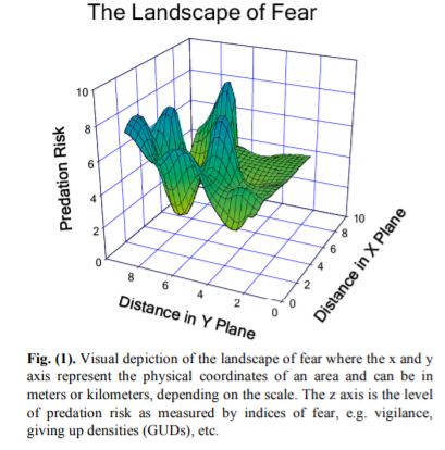
Laundre et al. (2010) present a visual representation of the landscape of fear (Fig. 1, reproduced below), where as an animal moves through space (represented as distance in meters or kilometers, for example), they also move through varying levels of predation risk. Environmental gradients (temperature, for example) tend to be much more stable across space in terrestrial ecosystems such as in the Yellowstone example from the paper. I wonder whether the same concept and visual depiction of a landscape of fear could be translated as risk across various environmental gradients, rather than geographic distances? In this proposed illustration, a landscape of fear would vary based on gradients of environmental conditions rather than geographic space. Such a shift in spatial reference —from geographic to environmental space—might make the model more applicable in the dynamic ocean ecosystems that we study.
What about cases when the predators we study become prey? One example we discussed was gray whales migrating from breeding lagoons in Mexico to feeding grounds in the Bering Sea. Mother-calf pairs hug the coastline tightly, by no means taking the most direct route between locations and adding considerable travel distance to their migration. The leading hypothesis is that mother gray whales take the coastal route to minimize the risk that their calves will fall prey to killer whale attacks. Are there other cases where the predators we study operate in a seascape of fear that we do not yet understand? Likely so, and the predators’ own seascape of fear may account for cases when we cannot explain predator distribution simply by their prey and their environment. To take this a step further, it might be beneficial not only to think of predation risk as only the potential to be eaten, but expand our definition to include human disturbance. While humans may not directly prey on marine predators, the disturbance from human activity in the ocean likely creates a layer of fear which animals must navigate, even in the absence of actual predation.
Our lively lab meeting discussion prompted me to look into how the landscape of fear model has been applied to the highly dynamic and intricate marine environment. In a study examining predator-prey dynamics of three species of marine mammals—bottlenose dolphins, harbor seals, and dugongs—Wirsing et al. (2007) found that in all three cases, the study species spent less time in more desirable prey patches or decreased riskier behavior in the presence of predators. Most studies in marine ecology are observational, as we rarely have the opportunity to manipulate our study system for experimental design and hypothesis testing. However, a study of coral reefs in the Florida Keys conducted by Catano et al. (2015) used fabricated predators—decoys of black grouper, a predatory fish—to investigate the influence of fear of predation on the reef system. What they found was that herbivorous fish consumed significantly less and fed at a much faster rate in the presence of this decoy predator. The grouper, even in decoy form, created a “reefscape of fear”, altering patterns in herbivory with potential ramifications for the entire ecosystem.
My takeaway from our discussion and my musings in this week’s blog post is that predator and prey distribution and behavior is highly interconnected. While predators distribute themselves to maximize their ability to find a meal, their prey respond accordingly by balancing finding a meal of their own with minimizing the risk that they will be eaten. Ecology is the study of an ecosystem, which means the questions we ask are complicated and hierarchical, and must be considered from multiple angles, accounting for biological, environmental, and behavioral elements to name a few. These challenges of studying ecosystems are simultaneously what make ecology fascinating, and exciting.
References:
Laundré, J. W., Hernández, L., & Ripple, W. J. (2010). The landscape of fear: ecological implications of being afraid. Open Ecology Journal, 3, 1-7.
Catano, L. B., Rojas, M. C., Malossi, R. J., Peters, J. R., Heithaus, M. R., Fourqurean, J. W., & Burkepile, D. E. (2016). Reefscapes of fear: predation risk and reef hetero‐geneity interact to shape herbivore foraging behaviour. Journal of Animal Ecology, 85(1), 146-156.
Wirsing, A. J., Heithaus, M. R., Frid, A., & Dill, L. M. (2008). Seascapes of fear: evaluating sublethal predator effects experienced and generated by marine mammals. Marine Mammal Science, 24(1), 1-15.