Last month I had the privilege to participate in the 2023 September Northern California Current (NCC) cruise onboard the NOAA RV Bell M. Shimada. These cruises are part of a long-term NOAA/NWFSC effort to study the NCC ecosystem and they have been taking place every February, May, and September since 2002. Thanks to a collaboration with NOAA (and more specifically the NCC cruise chief scientist Jennifer Fisher), the GEMM Lab has been able to put marine mammal observers on these cruises since 2018.
As a postdoc working on the OPAL project, I have been the main person in charge of processing and analyzing the cetacean data collected across the 10 (now 11!) cruises that the GEMM lab participated in. These data have played a paramount role in improving our understanding of rorqual whale (e.g., blue, humpback, fin) distribution and habitat use off the coast of Oregon (Derville et al., 2022) and assessing the resulting risk of entanglement in fishing gear that they face while migrating and feeding in our waters (Derville et al., 2023). But while I have been very involved in the data analysis side of things, up to now I had never been able to contribute to data collection for this project. First, I was working remotely at the height of the COVID pandemic and second, because the NCC cruises are onboard a NOAA vessel, they have strict limitations on non-US citizens participation. So, you can imagine how excited I was (as a French citizen) to finally set foot on the famous Bell M. Shimada that I had heard so many stories about!
The NCC cruises illustrate how valuable long-term ecosystem monitoring is. Station after station, miles surveyed after miles surveyed, little by little, we learn about the complex ecological relationships and changing patterns that shape life in the ocean. The data, the experience, and the memories accumulated over the years are a true legacy that I have felt very proud to be part of. Finally, being on this ship, I felt like I was walking in the path of so many of my friends who had held those same binoculars before. Florence Sullivan, who pioneered the GEMM Lab’s NCC cruise observer effort in the harsh winter weather of February 2018. Alexa Kownacki (May 2018, May 2019), whose detailed field notes I read years later with emotion and appreciation as they helped me figure out how the Seebird software used to collect data back then (and abandoned since!). Dawn Barlow (Sep 2018, Sep 2019, Sep 2020, May 2021, May 2022), our master observer who is said to be able to detect a whale’s blow 10 miles away in a 10-foot swell and Beaufort sea state 6, all while sipping an Affogato coffee. Clara Bird (Sep 2020, May 2022), who abandoned her beloved nearshore gray whales (twice!) to sail all the way to the NH-200 station (200 nautical miles from land!). Rachel Kaplan (May 2021, May 2022, Sep 2022), our jack of all trades who concurrently studies krill and whales, and by doing so probably broke the record of numbers of times running up and down between the flying bridge and the echosounder screen room down below. Renee Albertson (Sep 2022), a Marine Mammal Institute research associate who shared observations with Rachel until the cruise was cut short by an engine issue that led them to the docks of Seattle. And finally, Craig Hayslip (May 2023), who swapped his usual observer work on the United States Coast Guard’s helicopters as part of the OPAL project for two weeks onboard the Shimada.
What a team!
From left to right and top to bottom:Florence; Alexa; Dawn; Clara; Renee, Rachel and the rest of the science team including Jennifer Fisher and Anna Bolm; Craig; Rachel; and I!
The 11th NCC cruise with GEMM Lab observers onboard was equal to its predecessors as it provided a perfect combination of camaraderie, natural beauty, Pacific Northwest weather, and unexpected change of plans. After being delayed by one day, we discovered that a big storm system was coming upon us and would have us retreat to Yaquina Bay in Newport for 4 days! Overall, I spent 5 days surveying for marine mammals from the flying bridge, in conditions that went from a beautiful sunny Friday on September 22nd to an impressive Beaufort sea state 7 on the 29th. This experience was the king of weather in which it became particularly cool to be on a ship as big as the Shimada (63 m, 208 feet long!) that can withstand swell and wind better than any ship I had worked on before.
Overall, I observed 36 groups of cetaceans, including seven different species of dolphins and whales: one sperm whale, a possible Sei whale, several fin whales, blue whales, humpback whales, and pods of Pacific white-sided dolphins, Dall’s porpoises and common dolphins. Among the highlights of this cruise was the observation of several blue whales and humpback whales that seemed to be feeding on the western slope of the Heceta bank. My personal favorite memory was also to observe common dolphins -a species that despite its name is not that common (at least not in the nearshore environment) and that I had never seen before in my life! How magnificent and graceful they were… and how lucky was I to be part of this voyage.
From left to right, top to bottom: a CTD deployment from the Bell M. Shimada; a whale’s dinner? Krill collected with a bongo net during a previous cruise; a very distant yet unmistakable sperm whale dorsal knob; a group of common dolphins; a marine mammal observer’s work tools; a blue whale surfacing at dusk.
Derville, S., Barlow, D. R., Hayslip, C. E., & Torres, L. G. (2022). Seasonal, Annual, and Decadal Distribution of Three Rorqual Whale Species Relative to Dynamic Ocean Conditions Off Oregon, USA. Frontiers in Marine Science, 9, 868566. https://doi.org/10.3389/fmars.2022.868566
Derville, S., Buell, T. V, Corbett, K. C., Hayslip, C., & Torres, L. G. (2023). Exposure of whales to entanglement risk in Dungeness crab fishing gear in Oregon, USA, reveals distinctive spatio-temporal and climatic patterns. Biological Conservation, 109989. https://doi.org/10.1016/j.biocon.2023.109989
Baleen whales face a multitude of threats on a daily basis. The exposure to some of these threats can be assessed visually. For example, the presence of propeller scars on a whale are indicative that the individual was struck by a boat. However, there are some threats that are not easily detected from visual assessments. One of these threats is the ingestion of microparticles (MPs), which include microplastics and other anthropogenic debris. While MP research has entered its second decade and documentation of MPs in the marine environment is common, we still lack empirical information on the rates of MP ingestion by baleen whales and their prey. Hence, one of the objectives of the Coastal Oregon Zooplankton Investigation (COZI; read more about it in a previous blog), which GEMM Lab PI Leigh Torres led, was to determine to what extent Pacific Coast Feeding Group (PCFG) gray whales and their nearshore zooplankton prey are impacted by MPs. The results of this work were recently published in the journal Frontiers in Marine Science and I am going to summarize them for you here today.
A number of studies have documented MP ingestion in baleen whales, including in humpback (Besseling et al., 2015), fin (Fossi et al., 2012, 2014, 2016, 2017), Bryde’s, and sei whales (Zantis et al., 2022). The effects of ingesting MPs on baleen whales are theorized to include blockage of internal organs, mechanical damage of the digestive tract, false feeling of satiation (full from eating), and potentially leaching of toxicants depending on the length of the digestive period (Donohue et al., 2019; Hudak & Sette 2019; Zhu et al., 2019; Novillo et al., 2020). Despite the fact that MPs have been documented in a number of baleen whale species, there is still a lack of knowledge regarding MP ingestion rates by baleen whales from empirical data, although modeled estimates have been derived for a few species (Zantis et al., 2022; Kahane-Rapport et al., 2022). Basically, we know whales eat MPs because it has been detected in their stomachs, but we do not know how much MPs they consume. The COZI team therefore aimed to quantify baleen whale MP consumption rates from empirically counted MP loads in zooplankton prey and to look at MP exposure of baleen whales from “zoop to poop” (Figure 1).
Figure 1 Schematic depicting our “zoop to poop” approach. Taken from Torres et al., 2023.
In order to accomplish this aim, we used “zoop” and “poop” samples collected between 2017 to 2019 during the GEMM Lab’s long-term GRANITE (Gray whale Response to Ambient Noise Informed by Technology and Ecology) project. We analyzed MP loads in three prey zooplankton species found in nearshore Oregon waters (the amphipod Atylus tridens and the mysid shrimp Holmesimysis sculpta and Neomysis rayii), all of which are known PCFG gray whale prey (Hildebrand et al., 2021), as well as five fecal samples collected from four unique individual gray whales. While the field collection of these samples was led by the GEMM Lab, the processing and MP analysis was led by Dr. Susanne Brander and conducted by a number of undergraduate student workers. MP analysis is no easy feat as it involves many, many meticulous and time-intensive steps in order to get from a sample of gray whale prey or poop to a known number of MPs that the sample contained. The process involves (1) sorting and identifying the prey into the different species; (2) rinsing the individuals to ensure no external MPs are counted; (3) digesting the sample in potassium hydroxide (KOH) for 24-72 hours; (4) sieving and filtering the digested samples; (5) picking out suspected MPs from the filters and measuring them; (6) analyzing the suspected MPs to confirm chemical composition. On top of all of these steps, anyone working with the samples has to try and minimize potential MP contamination, which is not easy since MPs are practically everywhere, such as synthetic fibers from our clothes or microplastics that are floating around in the air.
Figure 2 Microparticle (MP) loads and morphotypes by zooplankton species. (A) the number of MPs per 1 gram per species, with the dotted line representing the average MP level in controls. (B) the proportion of MP morphotypes found in each zooplankton species. (C) the proportion of Fourier transform infrared (FTIR) spectroscopy categories of MPs found in each zooplankton species. The sample size for each sample is denoted above all columns.Taken fromTorres et al., 2023.
After many long years of lab work (COVID lab restrictions included), we are excited (and a little daunted) to share the results of this collaborative project with you. We detected MPs in all 26 zooplankton prey samples that we analyzed and found that the number of MPs in the three species were pretty similar, with an average of 4 MPs per gram of zooplankton (Figure 2). Over 50% of the 418 suspected MPs that we identified in the zooplankton samples were fibers. We also detected MPs in all five gray whale fecal samples that we analyzed. While we also detected fibers among the 37 suspected MPs pulled from the fecal samples, we found a higher proportion of larger MPs such as fragments and pellets in the “poop” samples, than we did in the “zoop” samples (Figure 3). We also tested some seawater samples as controls to see how the composition of MPs in seawater compared to that of zooplankton and gray whale feces. We found that seawater was dominated by fibers, similar to the zooplankton prey. This finding suggests that the larger MPs (e.g., fragments, pellets) that we found in gray whale feces must be coming from somewhere other than their prey and the ambient seawater. This led us to hypothesize that gray whales are likely exposed to MPs through two pathways, via (1) trophic transfer from their zooplankton prey and (2) indiscriminate consumption of ambient MPs in the benthos while foraging benthically (Figure 1).
Figure 3 Microparticle (MP) loads and morphotypes found in each of the five gray whale fecal samples analyzed. (A)the number of MPs per gram of fecal sample, with the dotted line representing the average MP level in controls. (B) the proportion of MP morphotypes found in each fecal sample. (C) the proportion of Fourier transform infrared (FTIR) spectroscopy categories of MPs found in each fecal sample. The sample size for each sample is denoted above all columns. Taken from Torres et al., 2023.
Next we wanted to estimate the daily ingestion rates of MPs by gray whales. For this estimation, we used our known values of zooplankton MP ingestion (from our analyzed samples) and extrapolated them using daily energetic needs of gray whales (i.e., how many calories does the whale need each day). The only published values of daily gray whale caloric needs are for pregnant and lactating females (Villegas-Amtmann et al., 2015, 2017), which is why we were only able to estimate daily MP ingestion rates for these two demographic groups. The numbers we calculated were rather staggering (and led us to double-, triple-, and quadruple-check our math) as we estimate that if a pregnant gray whale only ate the mysid N. rayii in a day, she would consume 9.55 million MP per day. We made these estimates for all three prey species that we analyzed as well as a “composite preyscape” (an average of the three prey species) and you can see all of those results in Table 1.
Table 1 Estimates of the number of microparticles (MPs) that a pregnant and lactating female gray whale consumes per day generated through extrapolation of results from this study (Microparticles per individual zooplankton; first row) to their daily energetic needs by zooplankton prey species from Hildebrand et al., 2021. Taken from Torres et al., 2023.
These results are frightening. They still are to me even though I have spent months with this knowledge after having done a lot of the data analysis for this project. I think it is particularly frightening to think about the fact that MPs are not the only anthropogenic threat that gray whales (and really any organism in the ocean) are exposed to. The good news is that you can do something to help reduce this threat in the oceans. Below are just a few suggestions of what you can do to reduce MP pollution to the environment:
A major source of pollution in the ocean comes from microfibers through our laundry (as you saw in our results). You can help stop this pathway by simply using a Cora Ball or installing a filter (such as this one) in your washing machine that captures microfleece & polyester fibers.
Minimize your use of single-use plastics. There are so many ways to do so including reuseable water bottles, travel mugs for coffee or tea, fabric totes as shopping bags, carry a set of utensils for takeout food, beeswax wraps instead of plastic wrap or sandwich bags.
Use public transport when possible as another huge source of microplastics comes from tire treads! This solution also helps reduce your carbon footprint.
References
Besseling E., Foekema E. M., Van Franeker J. A., Leopold M. F., Kühn S., Bravo Rebolledo E. L., et al. (2015). Microplastic in a macro filter feeder: humpback whale Megaptera novaeangliae. Mar. pollut. Bull. 95, 248–252. doi: 10.1016/j.marpolbul.2015.04.007
Donohue M. J., Masura J., Gelatt T., Ream R., Baker J. D., Faulhaber K., et al. (2019). Evaluating exposure of northern fur seals, callorhinus ursinus, to microplastic pollution through fecal analysis. Mar. pollut. Bull. 138, 213–221. doi: 10.1016/j.marpolbul.2018.11.036
Fossi M. C., Panti C., Guerranti C., Coppola D., Giannetti M., Marsili L., et al. (2012). Are baleen whales exposed to the threat of microplastics? a case study of the Mediterranean fin whale (Balaenoptera physalus). Mar. pollut. Bull. 64, 2374–2379. doi: 10.1016/j.marpolbul.2012.08.013
Fossi M. C., Coppola D., Baini M., Giannetti M., Guerranti C., Marsili L., et al. (2014). Large Filter feeding marine organisms as indicators of microplastic in the pelagic environment: the case studies of the Mediterranean basking shark (Cetorhinus maximus) and fin whale (Balaenoptera physalus). Mar. Environ. Res. 100, 17–24. doi: 10.1016/j.marenvres.2014.02.002
Fossi M. C., Marsili L., Baini M., Giannetti M., Coppola D., Guerranti C., et al. (2016). Fin whales and microplastics: the Mediterranean Sea and the Sea of cortez scenarios. Environ. pollut. 209, 68–78. doi: 10.1016/j.envpol.2015.11.022
Fossi M. C., Romeo T., Baini M., Panti C., Marsili L., Campani T., et al. (2017). Plastic debris occurrence, convergence areas and fin whales feeding ground in the Mediterranean marine protected area pelagos sanctuary: a modeling approach. Front. Mar. Sci. 4. doi: 10.3389/fmars.2017.00167
Hildebrand L., Bernard K. S., Torres L. G. (2021). Do gray whales count calories? comparing energetic values of gray whale prey across two different feeding grounds in the eastern north pacific. Front. Mar. Sci. 8. doi: 10.3389/fmars.2021.683634
Hudak C. A., Sette L. (2019). Opportunistic detection of anthropogenic micro debris in harbor seal (Phoca vitulina vitulina) and gray seal (Halichoerus grypus atlantica) fecal samples from haul-outs in southeastern Massachusetts, USA. Mar. pollut. Bull. 145, 390–395. doi: 10.1016/j.marpolbul.2019.06.020
Kahane-Rapport S. R., Czapanskiy M. F., Fahlbusch J. A., Friednlaender A. S., Calambokidis J., Hazen E. L., et al. (2022). Field measurements reveal exposure risk to microplastic ingestion by filter-feeding megafauna. Nat. Commun. 13, 6327. doi: 10.1038/s41467-022-33334-5
Novillo O., Raga J. A., Tomás J. (2020). Evaluating the presence of microplastics in striped dolphins (Stenella coeruleoalba) stranded in the Western Mediterranean Sea. Mar. pollut. Bull. 160, 111557. doi: 10.1016/j.marpolbul.2020.111557
Torres, L. G., Brander, S. M., Parker, J. I., Bloom, E. M., Norman, R., Van Brocklin, J. E., Lasdin, K.S., Hildebrand, L. (2023) Zoop to poop: assessment of microparticle loads in gray whale zooplankton prey and fecal matter reveal high daily consumption rates. Front. Mar. Sci. https://doi.org/10.3389/fmars.2023.1201078
Villegas-Amtmann S., Schwarz L. K., Sumich J. L., Costa D. P. (2015). A bioenergetics model to evaluate demographic consequences of disturbance in marine mammals applied to gray whales. Ecosphere 6, 1–19. doi: 10.1890/ES15-00146.1
Villegas-Amtmann S., Schwarz L. K., Gailey G., Sychenko O., Costa D. P. (2017). East Or west: the energetic cost of being a gray whale and the consequence of losing energy to disturbance. Endangered Species Res.34, 167–183. doi: 10.3354/esr00843
Zantis L. J., Bosker T., Lawler F., Nelms S. E., O’Rorke R., Constantine R., et al. (2022). Assessing microplastic exposure of large marine filter-feeders. Sci. Total Environ. 818, 151815. doi: 10.1016/j.scitotenv.2021.151815
Zhu J., Yu X., Zhang Q., Li Y., Tan S., Li D., et al. (2019). Cetaceans and microplastics: first report of microplastic ingestion by a coastal delphinid, Sousa chinensis. Sci. Total Environ. 659, 649–654. doi: 10.1016/j.scitotenv.2018.12.389
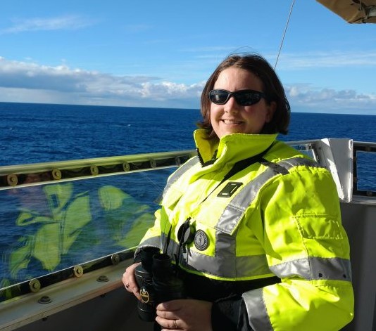
Hello from Palmer Station, Antarctica! I’ve spent the last five months here in a kind of parallel universe to that of my normal life in Oregon. It’s spring here at the Western Antarctic Peninsula (WAP), and since May I’ve been part of a team studying Antarctic krill (Euphausia superba) – a big change from the Oregon species I typically study, and one that has already taught me so much.
I am here as part of a project titled “The Omnivore’s Dilemma: The effect of autumn diet on winter physiology and condition of juvenile Antarctic krill”. Through at-sea fieldwork and experiments in the lab, we have spent this field season investigating how climate-driven changes in diet impact juvenile and adult krill health during the long polar night. Winter is a crucial time for krill survival and recruitment, and an understudied season in this remote corner of the world.
Within this field season, we have been part of two great research cruises along the WAP, and spent the rest of the time at Palmer Station, running long-term experiments to learn how diet influences krill winter growth and development. The time has passed incredibly fast, and it’s hard to believe that we’ll be heading home in just a couple weeks.
There have been so many wonderful parts to our time here. While at sea, I was constantly aware that each new bay and fjord we sampled was one of the most beautiful places I would ever have the privilege to visit. I was also surprised and thrilled by the number of whales we saw – I recorded over one hundred sightings, including humpbacks, minke, and killer whales. As consumed as I was by looking for whales during the few hours of daylight, it was also rewarding to broaden my marine mammal focus and learn about another krill predator, the crabeater seal, from a great team researching their ecology and physiology.
In between our other work, I have been processing active acoustic (echosounder) data collected during a winter 2022 cruise that visited many of the same regions of the WAP. Antarctic krill have been much more thoroughly studied than the main krill species that occur off the coast of Oregon, Euphausia pacifica and Thysanoessa spinifera, and it has been amazing to draw upon this large body of literature.
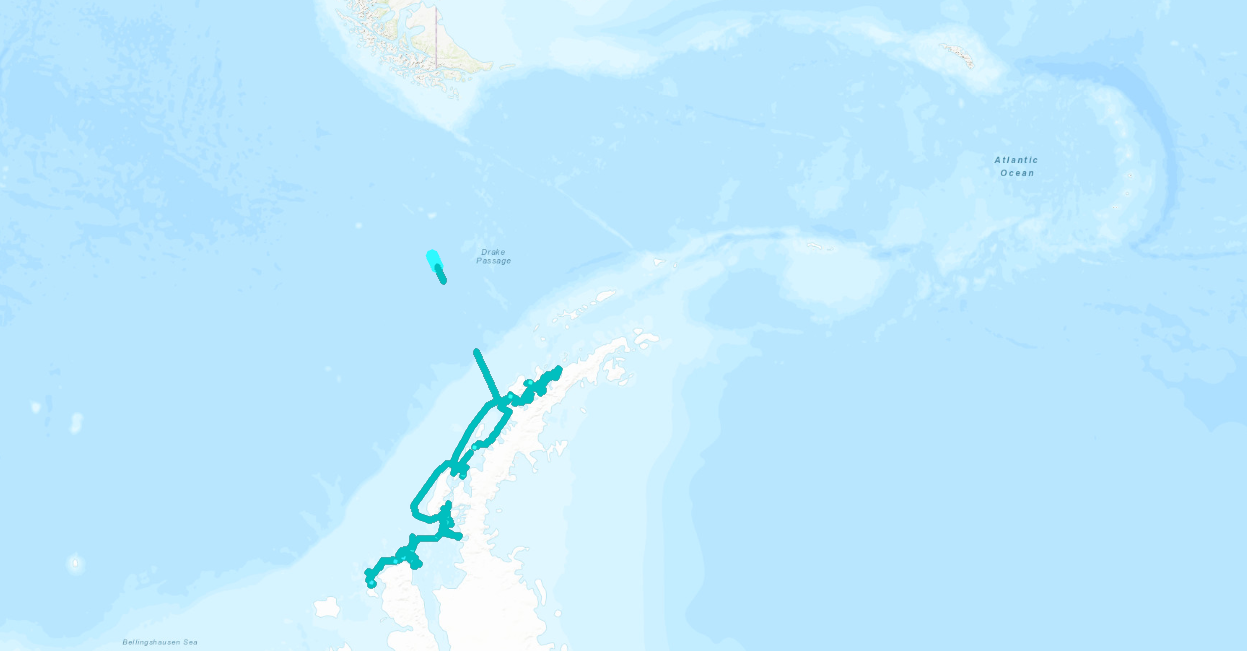
Figure 2. The active acoustic data I’m working with from the Western Antarctic Peninsula, pictured here, was collected along a wiggly cruise track in 2022, giving me the opportunity to learn how to process this type of survey data and appreciate the ways in which a ship’s movements translate to data analysis.
Working with a new flavor of echosounder data has presented me with puzzles that are teaching me to navigate different modes of data collection and their analytical implications, such as for the cruise track data above. I’ll never take data collected along a standardized grid for granted again!
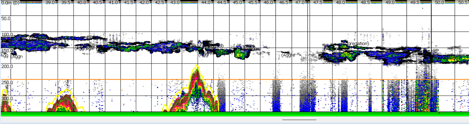
I’ve also learned new techniques that I am excited to apply to my research in the Northern California Current (NCC) region. For example, there are two primary different ways of detecting krill swarms in echosounder data: by comparing the results of two different acoustic frequencies, and by training a computer algorithm to recognize swarms based on their dimensions and other characteristics. After trying a few different approaches with the Antarctic data this season, I developed a way to combine these techniques. In the resulting dataset, two different methods have confirmed that a given area represents krill, which gives me a lot of confidence in it. I’m looking forward to applying this technique to my NCC data, and using it to assess some of my next research questions.
Figure 3. A combination of krill detection techniques selected these long krill aggregations off the coast of the Western Antarctic Peninsula (WAP).
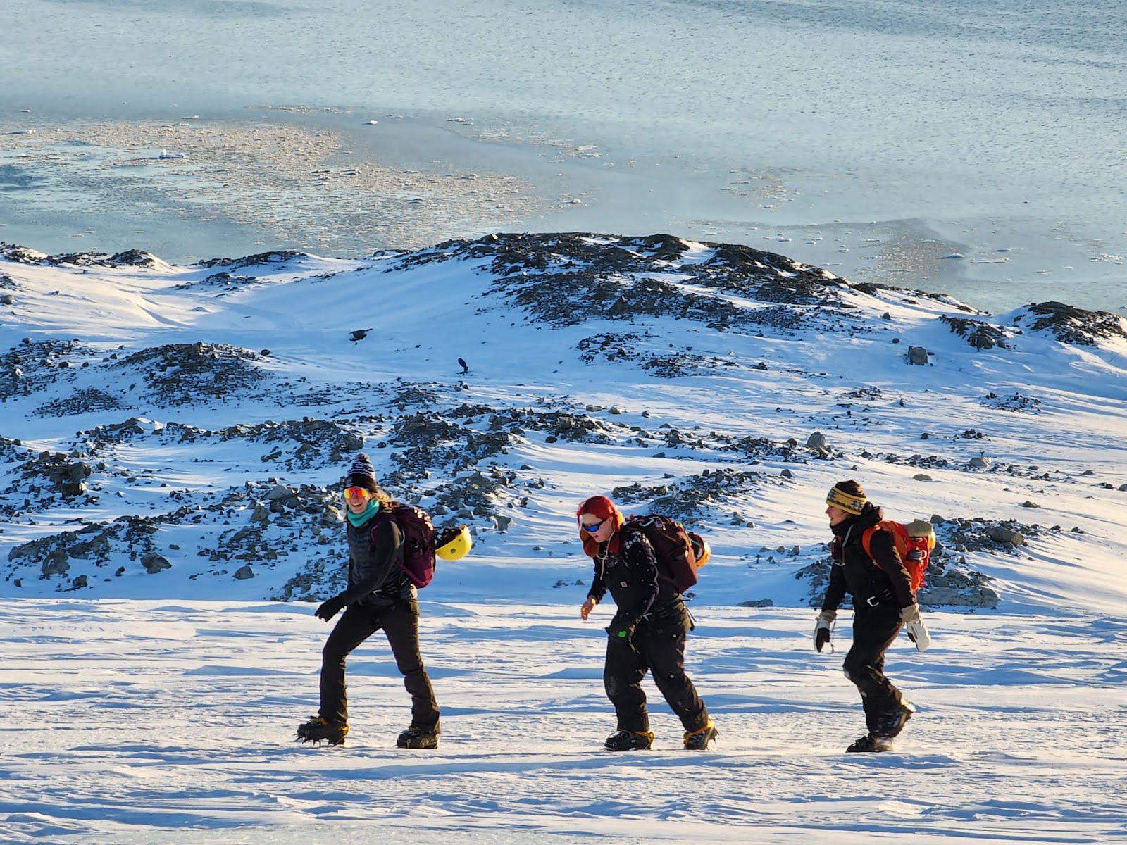
Throughout it all, the highlight of this season has been being part of an amazing field team. I’m here with Kim Bernard (as a co-advised student, I refer to Kim as my “krill advisor” and Leigh as my “whale advisor”), and undergraduate Abby Tomita, who just started her senior year at OSU remotely from Palmer. From nights full of net tows to busy days in the lab, we’ve become a well-oiled machine, and laughed a lot along the way. Working with the two of them makes me sure that we’ll be able to best any difficulties that come up.
Now, our next challenge is wrapping up our last labwork, packing up equipment and samples, and getting ready to say goodbye. Leaving this wild, remote place is always heartbreaking – you never really know if you’ll be back. But there’s a lot to look forward to as we journey north, too: I can’t wait to hug my family and friends, eat a salad, and drive out to Newport to see the GEMM Lab. I’m excited to head back to the world with everything I’ve learned here, and to keep working.
Figure 4. Kim (left), Abby (middle), and I (right) hike on the Marr Ice Piedmont during a gorgeous day off.
When I wrote my first blog a year ago, I was just starting to dig into the field work and data analysis I had loftily proposed for my graduate degree. Now I am writing to you as a new Master of Science! A little more than a month ago, I successfully defended my thesis research where I used the data from minimally invasive high-resolution accelerometry suction cup tags deployed by the GEMM Lab to estimate the relative energetic cost of different foraging behaviors (see my first blog) of Pacific Coast Feeding Group (PCFG) gray whales that forage during summer months off the coast of Oregon. I learned a lot of new skills through this research project and am excited to share some of my odyssey with you.
To start, I want to highlight the technology that made this work possible: the high-resolution accelerometry suction cup tags. These suction cup tags not only record fine scale data about the whale’s movement and behavior from inertial sensors like accelerometers, magnetometers and gyroscopes, the tags also incorporate video and audio data to record what the whale is seeing and hearing in its environment. I used the data from these tags to achieve two research objectives relating to 1) describing foraging behavior of PCFG gray whales and 2) estimating the relative energetic cost of these behaviors.
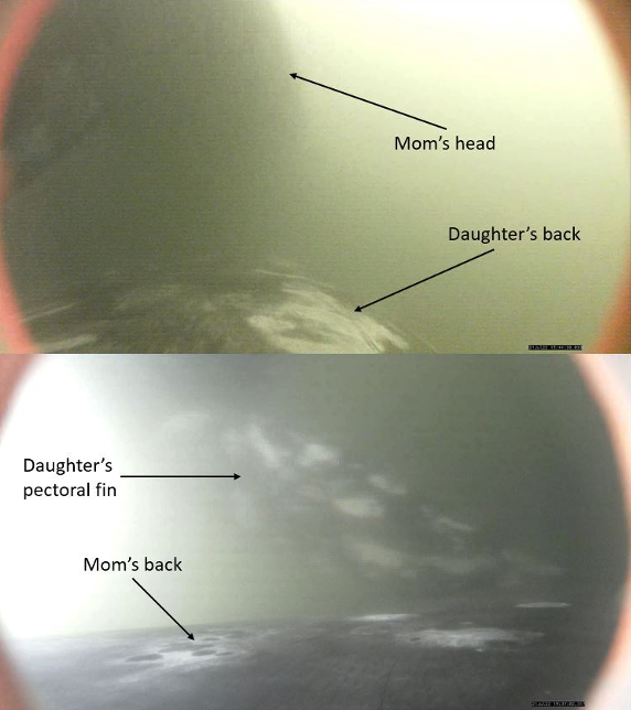
Through the hard work of the GEMM Lab field team and collaborators John Calambokidis and Dr. Dave Cade, 10 of these high-resolution accelerometry tags were deployed to collect approximately 91.5 hours of data from PCFG gray whales. Excitingly, two of these tags were deployed on a known mother-daughter pair on the same day. The mother and her 8-year-old daughter were even observed foraging together while tagged later in the day and recorded each other while feeding (Figure 1)!
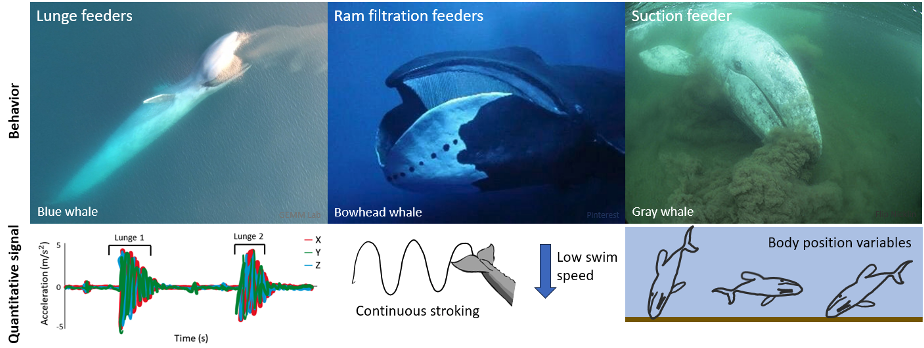
My first research objective was to quantitatively describe the foraging behaviors of PCFG gray whales. These quantitative descriptions exist for other baleen whale foraging behaviors, such as the lunge feeding behavior of rorqual whales (e.g., humpback, fin, and blue whales) where large mouthfuls of prey are engulfed, or the ram filtration feeding of bowhead and right whales where water is filtered for prey as the whale swims along with its mouth open. High-resolution accelerometry tag data has found that a strong acceleration signal is useful for detecting lunges (Goldbogen et al., 2013) and continuous fluking paired with low swim speeds signal the occurrence of ram filtration feeding (Simon et al., 2009). However, gray whales are the only baleen whales to use suction feeding behavior where the whale rolls to one side and sucks up water to filter for prey. Beyond describing side preferences when performing suction feeding (Woodward & Winn, 2006), this unique foraging behavior of gray whales lacks quantitative descriptions. My thesis works to add quantitative descriptions of gray whale suction feeding to the existing descriptions of baleen whale foraging behavior using high-resolution tag data. Based on previous drone focal follows that qualitatively describe gray whale foraging behaviors (Torres et al., 2018), I hypothesized that body position variables would be important for quantitatively describing PCFG gray whale foraging tactics using tag data. I anticipated that the signals of gray whale suction feeding behavior would be different from the signals of lunge and ram filtration feeding performed by other species of baleen whales (Figure 2).
Figure 1. Snapshots from the video footage of high-resolution accelerometry suction cup tags deployed on a mother-daughter pair of whales foraging together. The top photo is from the tag deployed on the daughter filming the mother, and the bottom photo is from the tag deployed on the mother filming the daughter.
Figure 2. Quantitative descriptions of foraging behaviors for different baleen whale feeding mechanisms. The left panel indicates the strong acceleration signal used to detect lunges of rorquals (e.g., humpback, fin, and blue whales). The acceleration figure is adapted from Izadi et al., (2022). The middle panel shows the continuous fluking and low swim speed signal for ram filtration feeding of bowheads (Simon et al., 2009). The right panel indicates the hypothesized importance of body position variables when quantitatively describing the unique suction feeding behavior of gray whales (my thesis).
My second objective was to estimate the relative energetic cost of PCFG gray whale foraging behaviors. Previous research has estimated the energetic cost of gray whale broad state behaviors (e.g., transit, search, and forage) using respiration rates (Sumich, 1986). However, respiration rates are difficult to use when estimating the energetic cost of fine scale behaviors, like the precise foraging tactics performed within a dive. Therefore, I calculated biologging-derived proxies of energy expenditure from the tag data such as stroke rate (i.e., the frequency of the whale’s fluke beats) and Overall Dynamic Body Acceleration (ODBA; i.e., the total body movement of the whale) to estimate the relative energetic cost of three different PCFG gray whale foraging tactics: benthic dig, headstand, and side swim. To put these energy expenditure proxies into a human example, if you were walking, your stroke rate would be the frequency of your steps and your ODBA would be all the acceleration of your body including your legs moving with each step, your swinging arms, and turning head. Stroke rate and ODBA are common proxies of energy expenditure that are easily calculated from biologging tag data and have been linked to metabolic rate in many species, including bottlenose dolphins (Allen et al., 2022) and fur seals (Jeanniard-Du-Dot et al., 2016).
When comparing these two proxies of energy expenditure between PCFG gray whale foraging tactics, I expected that the benthic dig foraging behavior would be the least energetically costly compared to the other PCFG foraging tactics. Benthic digs occur when the whale is rolled onto its side and plows through the sediment to suction up prey while leaving feeding pits on the seafloor. Benthic digs are assumed to be the primary foraging tactic of the majority of the gray whale population (Nerini, 1984) that feed in the Arctic and sub-Arctic region where gray whales must dive deeper to reach their prey in the bottom sediments, making it likely that a lower energetic cost of foraging motivates the higher use of this foraging tactic. Excitingly, preliminary results indicate that these three gray whale foraging tactics have different energy expenditures, which can potentially help explain patterns of behavior choice and tactic usage between different groups of gray whales. My thesis research is a foundational step toward better understanding gray whale foraging energetics by providing a means to assess prey requirements and inform management policies to reduce threats facing the PCFG gray whales. For example, previous work has shown that vessel disturbance reduces the searching time (Sullivan & Torres, 2018) and increases the stress levels (Lemos et al., 2022) of PCFG gray whales. My work builds on this by demonstrating an elevated energetic cost of some foraging tactics that could be used to support increasing the distance requirements between vessels and feeding PCFG whales as a way to reduce the energetic impact of vessel disturbance (Figure 3). Additionally, differences in energetic cost of foraging behaviors may help inform potential risks posed by changes in prey quality and quantity for gray whales using different foraging tactics.
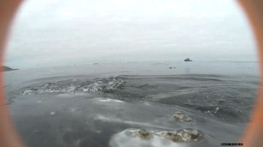
Figure 3. Snapshot from the video footage of a high-resolution accelerometry suction cup tag deployed on a PCFG gray whale showing the high number of vessels present during a surfacing following a foraging dive. The energetic cost of foraging behaviors found in my thesis might suggest that increasing distance between vessels and forging whales could reduce the energetic impacts of vessel disturbance.
Overall, I am so grateful for my Master’s experience. I had the opportunity to work with amazing scientists that taught me many valuable skills and lessons that I will take with me as I move onto the next phase of my career. Throughout my degree I’ve had a lot of “firsts” and I am excited to embark on another as I prepare my first manuscripts for publication!
References:
Allen, A. S., Read, A. J., Shorter, K. A., Gabaldon, J., Blawas, A. M., Rocho-Levine, J., & Fahlman, A. (2022). Dynamic body acceleration as a proxy to predict the cost of locomotion in bottlenose dolphins. Journal of Experimental Biology, 225(4). https://doi.org/10.1242/jeb.243121
Goldbogen, J. A., Friedlaender, A. S., Calambokidis, J., McKenna, M. F., Simon, M., & Nowacek, D. P. (2013). Integrative approaches to the study of baleen whale diving behavior, feeding performance, and foraging ecology. BioScience, 63(2), 90–100. https://doi.org/10.1525/bio.2013.63.2.5
Izadi, S., Aguilar de Soto, N., Constantine, R., & Johnson, M. (2022). Feeding tactics of resident Bryde’s whales in New Zealand. Marine Mammal Science, 1–14. https://doi.org/10.1111/mms.12918
Jeanniard-Du-Dot, T., Trites, A. W., Arnould, J. P. Y., Speakman, J. R., & Guinet, C. (2016). Flipper strokes can predict energy expenditure and locomotion costs in free-ranging northern and Antarctic fur seals. Scientific Reports, 6. https://doi.org/10.1038/srep33912
Lemos, L. S., Haxel, J. H., Olsen, A., Burnett, J. D., Smith, A., Chandler, T. E., Nieukirk, S. L., Larson, S. E., Hunt, K. E., & Torres, L. G. (2022). Effects of vessel traffic and ocean noise on gray whale stress hormones. Scientific Reports, 12(1). https://doi.org/10.1038/s41598-022-14510-5
Nerini, M. (1984). A review of gray whale feeding ecology. In M. Lou Jones, S. L. Swartz, & S. Leatherwood (Eds.), The gray whale: Eschrichtius robustus (pp. 423–450). Academic Press. https://doi.org/10.1016/B978-0-08-092372-7.50024-8
Simon, M., Johnson, M., Tyack, P., & Madsen, P. T. (2009). Behaviour and kinematics of continuous ram filtration in bowhead whales (Balaena mysticetus). Proceedings of the Royal Society B: Biological Sciences, 276(1674), 3819–3828. https://doi.org/10.1098/rspb.2009.1135
Sullivan, F. A., & Torres, L. G. (2018). Assessment of vessel disturbance to gray whales to inform sustainable ecotourism. Journal of Wildlife Management, 82(5), 896–905. https://doi.org/10.1002/jwmg.21462
Sumich, J. L. (1986). Latitudinal distribution, calf growth and metabolism, and reproductive energetics of gray whales, Eschrichtius robustus. Oregon State University.
Torres, L. G., Nieukirk, S. L., Lemos, L., & Chandler, T. E. (2018). Drone up! Quantifying whale behavior from a new perspective improves observational capacity. Frontiers in Marine Science, 5. https://doi.org/10.3389/fmars.2018.00319
Woodward, B. L., & Winn, J. P. (2006). Apparent lateralized behavior in gray whales feeding off the Central British Columbia coast. Marine Mammal Science, 22(1), 64–73. https://doi.org/10.1111/j.1748-7692.2006.00006.x
Sagar Karki, Master’s student in the Computer Science Department at Oregon State University
What beasts? Good question! We are talking about gray whales in this article but honestly we can tweak the system discussed in this blog a little and make it usable for other marine animals too.
Understanding the morphology, such as body area and length, of wild animals and populations can provide important information on animal behavior and health (check out postdoc Dr. KC Bierlich’s post on this topic). Since 2015, the GEMM Lab has been flying drones over whales to collect aerial imagery to allow for photogrammetric measurements to gain this important morphological data. This photogrammetry data has shed light on multiple important aspects of gray whale morphology, including the facts that the whales feeding off Oregon are skinnier [1] and shorter [2] than the gray whales that feed in the Arctic region. But, these surprising conclusions overshadow the immense, time-consuming labor that takes place behind the scenes to move from aerial images to accurate measurements.
To give you a sense of this laborious process, here is a quick run through of the methods: First the 10 to 15 minute videos must be carefully watched to select the perfect frames of a whale (flat and straight at the surface) for measurement. The selected frames from the drone imagery are then imported into MorphoMetriX, which is a custom software developed for photogrammetry measurement [1]. MorphoMetriX is an interactive application that allows an analyst to manually measure the length by clicking points along the centerline of the whale’s body. Based on this line, the whale is divided into a set of sections perpendicular to the centerline, these are used to then measure widths along the body. The analyst then clicks border points at the edge of the whale’s body to delineate the widths following the whale’s body curve. MorphoMetriX then generates a file containing the lengths and widths of the whale in pixels for each measured image. The length and widths of whales are converted from pixels to metric units using a software called CollatriX [4] and this software also calculates metrics of body condition from the length and width measurements.
While MorphoMetriX [3] and CollatriX [4] are both excellent platforms to facilitate these photogrammetry measurements, each measurement takes time, a keen eye, and attention to detail. Plus, if you mess up one step, such as an incorrect length or width measurement, you have to start from the first step. This process is a bottleneck in the process of obtaining important morphology data on animals. Can we speed this process up and still obtain reliable data?
What if we can apply automation using computer vision to extract the frames we need and automatically obtain measurements that are as accurate as humans can obtain? Sounds pretty nice, huh? This is where I come into the picture. I am a Master’s student in the Computer Science Department at OSU, so I lack a solid background in marine science, but bring to the table my skills as a computer programmer. For my master’s project, I have been working in the GEMM Lab for the past year to develop automated methods to obtain accurate photogrammetry measurements of whales.
We are not the first group to attempt to use computers and AI to speed up and improve the identification and detection of whales and dolphins in imagery. Researchers have used deep learning networks to speed up the time-intensive and precise process of photo-identification of individual whales and dolphins [5], allowing us to more quickly determine animal location, movements and abundance. Millions of satellite images of the earth’s surface are collected daily and scientists are attempting to utilize these images to benefit marine life by studying patterns of species occurrence, including detection of gray whales in satellite images using deep learning [6]. There has also been success using computer vision to identify whale species and segment out the body area of the whales from drone imagery [7]. This process involves extracting segmentation masks of the whale’s body followed by length extraction from the mask. All this previous research shows promise for the application of computer vision and AI to assist with animal research and conservation. As discussed earlier, the automation of image extraction and photogrammetric measurement from drone videos will help researchers collect vital data more quickly so that decisions that impact the health of whales can be more responsive and effective.For instance, photogrammetry data extracted from drone images can diagnose pregnancy of the whales [8], thus automation of this information could speed up our ability to understand population trends.
Computer vision and natural language processing fields are growing exponentially. There are new foundation models like ChatGPT that can do most of the natural language understanding and processing tasks. Foundational models are also emerging for computer vision tasks, such as “the segment anything model” from Meta. Using these foundation models along with other existing research work in computer vision, we have developed and deployed a system that automates the manual and computational tasks of MorphoMetriX and CollatriX systems.
This system is currently in its testing and monitoring phase, but we are rapidly moving toward a publication to disseminate all the tools developed, so stay tuned for the research paper that will explain in detail the methodologies followed on data processing, model training and test results. The following images give a sneak peak of results. Each image illustrates a frame from a drone video that was identified and extracted through automation, followed by another automation process that identified important points along the whale’s body and curvature. The user interface of the system aims to make the user experience intuitive and easy to follow. The deployment is carefully designed to run on different hardwares, with easy monitoring and update options using the latest open source frameworks. The user has to do just two things. First, select the videos for analysis. The system then generates potential frames for photogrammetric analysis (you don’t need to watch 15 mins of drone footage!). Second, the user selects the frame of choice for photogrammetric analysis and waits for the system to give you measurements. Simple! Our goal is for these softwares to be a massive time-saver while still providing vital, accurate body measurements to the researchers in record time. Furthermore, an advantage of this approach is that researchers can follow the methods in our to-be-soon-published research paper to make a few adjustments enabling the software to measure other marine species, thus expanding the impact of this work to many other life forms.
A sneak peek of the results. Each image illustrates a frame from a drone video that was identified and extracted through automation, followed by another automation process that identified important points along the whale’s body and curvature.
Did you enjoy this blog? Want to learn more about marine life, research, and conservation? Subscribe to our blog and get a weekly message when we post a new blog. Just add your name and email into the subscribe box below.
References
Torres LG, Bird CN, Rodríguez-González F, Christiansen F, Bejder L, Lemos L, Urban R J, Swartz S, Willoughby A, Hewitt J, Bierlich K (2022) Range-Wide Comparison of Gray Whale Body Condition Reveals Contrasting Sub-Population Health Characteristics and Vulnerability to Environmental Change. Front Mar Sci 910.3389/fmars.2022.867258
Bierlich KC, Kane A, Hildebrand L, Bird CN, Fernandez Ajo A, Stewart JD, Hewitt J, Hildebrand I, Sumich J, Torres LG (2023) Downsized: gray whales using an alternative foraging ground have smaller morphology. Biol Letters 19:20230043 doi:10.1098/rsbl.2023.0043
Torres et al., (2020). MorphoMetriX: a photogrammetric measurement GUI for morphometric analysis of megafauna. Journal of Open Source Software, 5(45), 1825, https://doi.org/10.21105/joss.01825
Bird et al., (2020). CollatriX: A GUI to collate MorphoMetriX outputs. Journal of Open Source Software, 5(51), 2328, https://doi.org/10.21105/joss.02328
Patton, P. T., Cheeseman, T., Abe, K., Yamaguchi, T., Reade, W., Southerland, K., Howard, A., Oleson, E. M., Allen, J. B., Ashe, E., Athayde, A., Baird, R. W., Basran, C., Cabrera, E., Calambokidis, J., Cardoso, J., Carroll, E. L., Cesario, A., Cheney, B. J. … Bejder, L. (2023). A deep learning approach to photo–identification demonstrates high performance on two dozen cetacean species. Methods in Ecology and Evolution, 00, 1–15. https://doi.org/10.1111/2041-210X.14167
Green, K.M., Virdee, M.K., Cubaynes, H.C., Aviles-Rivero, A.I., Fretwell, P.T., Gray, P.C., Johnston, D.W., Schönlieb, C.-B., Torres, L.G. and Jackson, J.A. (2023), Gray whale detection in satellite imagery using deep learning. Remote Sens Ecol Conserv. https://doi.org/10.1002/rse2.352
Gray, PC, Bierlich, KC, Mantell, SA, Friedlaender, AS, Goldbogen, JA, Johnston, DW. Drones and convolutional neural networks facilitate automated and accurate cetacean species identification and photogrammetry. Methods Ecol Evol. 2019; 10: 1490–1500. https://doi.org/10.1111/2041-210X.13246
Fernandez Ajó A, Pirotta E, Bierlich KC, Hildebrand L, Bird CN, Hunt KE, Buck CL, New L, Dillon D, Torres LG (2023) Assessment of a non-invasive approach to pregnancy diagnosis in gray whales through drone-based photogrammetry and faecal hormone analysis. Royal Society Open Science 10:230452
Mariam Alsaid, University of California Berkeley, GEMM Lab REU Intern
My name is Mariam Alsaid and I am currently a 5th year undergraduate transfer student at the University of California, Berkeley. Growing up on the small island of Bahrain, I was always minutes away from the water and was enraptured by the creatures that lie beneath the surface. Despite my long-standing interest in marine science, I never had the opportunity to explore it until just a few months ago. My professional background up until this point was predominantly in soil microbiology through my work with Lawrence Berkeley National Laboratory, and I was anxious about how I would switch directions and finally be able to pursue my main passion. For this reason, I was thrilled by my acceptance into the OSU Hatfield Marine Science Center’s REU program this year, which led to my exciting collaboration with the GEMM Lab. It was kind of a silly transition to go from studying bacteria, one of the smallest organisms on earth, to whales, who are the largest.
My project this summer focused on sei whale acoustic occurrence off the coast of Oregon. “What’s a sei whale?” is a question I heard a lot throughout the summer and is one that I had to Google myself several times before starting my internship. Believe it or not, sei whales are the third largest rorqual in the world but don’t get much publicity because of their small population sizes and secretive behavior. The commercial whaling industry of the 19th and 20th centuries did a number on sei whale populations globally, rendering them endangered. In consequence, little research has been conducted on their global range, habitat use, and behavior since the ban of commercial whaling in 1986 (Nieukirk et al. 2020). Additionally, sei whales are relatively challenging to study because of their physical similarities to the fin whale, and acoustic similarities to other rorqual vocalizations, most notably blue whale D-calls and fin whale 40 Hz calls. As of today, published literature indicates that sei whale acoustic presence in the Pacific Ocean is restricted to Antarctica, Chile, Hawaii, and possibly British Columbia, Canada (Mcdonald et al. 2005; Espanol-Jiminez et al. 2019; Rankin and Barlow, 2012; Burnham et al. 2019). The idea behind this research project was sparked by sparse visual sightings of sei whales by research cruises conducted by the Marine Mammal Institute (MMI) in recent years (Figure 1). This raised questions about if sei whales are really present in Oregon waters (and not just misidentified fin whales) and if so, how often?
Figure 1. Map of sei whale visual sightings off the coast of Oregon, colored by MMI Lab research cruise, and the location of the hydrophone at NH45 (white star).
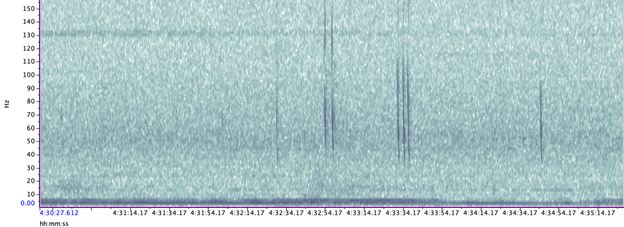
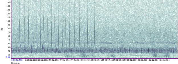
A hydrophone, which is a fancy piece of equipment that records continuous underwater sound, was deployed 45 miles offshore of Newport, OR between October of 2021 and December of 2022. My role this summer was to use this acoustic data to determine whether sei whales are hanging out in Oregon or not. Acoustic data was analyzed using the software Raven Pro, which allowed me to visualize sound in the form of spectrograms (Fig. 2). From there, my task was to select signals that could potentially be sei whale calls. It was a hurdle familiarizing myself with sei whale vocalizations while also keeping in mind that other species (e.g., blue and fin whales) may produce similar sounding (and looking in the spectrograms) calls. For this reason, I decided to establish confidence levels based on published sei whale acoustic research that would help me classify calls with less bias. Vocalizations produced by sei whales are characterized by low frequency, broadband, downsweeps. Sei whales can be acoustically distinguished from other whales because of their tendency to produce uniform groups of calls (typically in doublets and triplets) in a short timeframe. This key finding allowed me to navigate the acoustic data with more ease.
The majority of the summer was spent slowly scanning through the months of data at 5-minute increments. As you can imagine, excitement varied by day. Some days I would find insanely clear signals of blue, fin, and humpback whales and other days I would find nothing. The major discovery and the light at the end of the tunnel was the SEI WHALES!!! I detected numerous high quality sei whale calls throughout the study period with peaks in October and November (but a significantly higher peak in occurrence in 2022 versus 2021). I also encountered a unique vocalization type in fall of 2022, consisting of a very long series of repeated calls that we called “multiplet”, rather than doublets or triplets that is more typical of sei whales (Fig. 3). Lastly, I found no significant diel pattern in sei whale vocalization, indicating that these animals call at any hour of the day. More research needs to go into this project to better estimate sei whale occurrence and understand their behavior in Oregon but this preliminary work provides a great baseline into what sei whales sound like in this part of the world. In the future, the GEMM lab intends on implementing more hydrophone data and work on developing an automated detection system that would identify sei whale calls automatically.
Figure 2. Spectrogram of typical sei whale calls detected in acoustic dataFigure 3. Spectrogram of unique sei whale multiplet call type
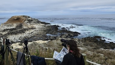
Figure 4. My first time conducting fieldwork! I spent a few mornings assisting Dr. Rachel Orben’s group in surveying murre and cormorant nests (thanks to my good friend Jacque McKay :))
My experience this summer was so formative for me. As someone who has been an aspiring marine biologist for so long, I am so grateful for my experience working with the GEMM Lab alongside incredible scientists who are equally passionate about studying the mysteries of the ocean. This experience has also piqued my interest in bioacoustics and I plan on searching for other opportunities to explore the field in the future. Aside from growing professionally, I learned that I am more capable of tackling and overcoming obstacles than I had thought. I was afraid of entering a field that I knew so little about and was worried about failing and not fitting in. My anxieties were overshadowed by the welcoming atmosphere at Hatfield and I could not have asked for better people to work with. As I was searching for sei whale calls this summer, I suppose that I was also unintentionally searching for my voice as a young scientist in a great, blue field.
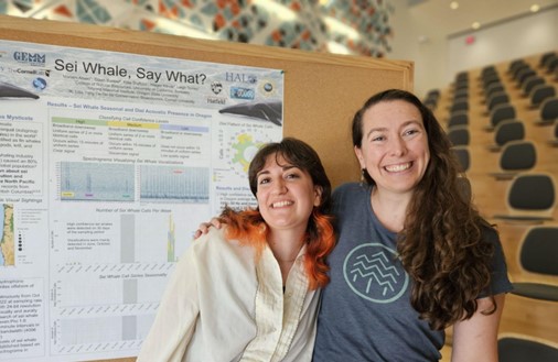
Figure 5. My mentor, Dr. Dawn Barlow, and I with my research poster at the Hatfield Marine Science Center Coastal Intern Symposium
Did you enjoy this blog? Want to learn more about marine life, research, and conservation? Subscribe to our blog and get a weekly alert when we make a new post! Just add your name into the subscribe box below!
References:
Nieukirk, S. L., Mellinger, D. K., Dziak, R. P., Matsumoto, H., & Klinck, H. (2020). Multi-year occurrence of sei whale calls in North Atlantic polar waters. The Journal of the Acoustical Society of America, 147(3), 1842–1850.https://doi.org/10.1121/10.0000931
McDonald, M. A., Calambokidis, J., Teranishi, A. M., & Hildebrand, J. A. (2001). The acoustic calls of blue whales off California with gender data. The Journal of the Acoustical Society of America, 109(4), 1728–1735.https://doi.org/10.1121/1.1353593
Español-Jiménez, S., Bahamonde, P. A., Chiang, G., & Häussermann, V. (2019). Discovering sounds in Patagonia: Characterizing sei whale (<i>Balaenoptera borealis</i>) downsweeps in the south-eastern Pacific Ocean. Ocean Science, 15(1), 75–82.https://doi.org/10.5194/os-15-75-2019
Rankin, S., & Barlow, J. (2007). VOCALIZATIONS OF THE SEI WHALE BALAENOPTERA BOREALIS OFF THE HAWAIIAN ISLANDS. Bioacoustics, 16(2), 137–145.https://doi.org/10.1080/09524622.2007.9753572
Burnham, R. E., Duffus, D. A., & Mouy, X. (2019). The presence of large whale species in Clayoquot Sound and its offshore waters. Continental Shelf Research, 177, 15–23.https://doi.org/10.1016/j.csr.2019.03.004
Celest Sorrentino, Research Technician, Geospatial Ecology of Marine Megafauna Lab
Hello again GEMM Lab family. I write to you exactly a year after (okay maybe 361 days after but who’s counting…) from my previous blog post describing my 2022 summer working in the GEMM Lab as an NSF REU intern. Since then, so much has changed, and I can’t wait to fill you in on it.
In June I walked across the commencement stage at UC Santa Barbara, earning my BS in Ecology, Evolution, and Marine Biology and my minor in Italian language. A week later, I packed my bags and headed straight back to the lukewarm beaches of Newport, Oregon as a Research Technician in the GEMM Lab. I am incredibly fortunate to have been invited back to the OSU Marine Mammal Institute to lend a hand analyzing drone footage of gray whales collected back in March 2023 when Leigh and Clara went down to Baja California, as mentioned previously in Clara’s blog.
Fig. 1. View from the top! (of the bridge at Yaquina Bay Bridge in Newport, OR)
During my first meeting with Clara at the beginning of the summer we discussed that a primary goal of my position was to process all the drone footage collected in Baja so that the generated video clips could be later used in other analytical software such as BORIS and SLEAP A.I. Given my previous internships and past summer project, this video processing is familiar to me. My initial thoughts were:
Sweet! Watch drone footage, pop in some podcasts, note down when I see whales, let’s do this!*
Like any overly eager 23-year-old, I might have mentally cracked open a Celsius and kicked my feet up too soon. We added another layer to the goal: develop an ethogram – which requires me to identify and define the behaviors that the gray whales appear to be demonstrating within the videos (more on ethogram development in Clara’s previous blog.) This made me nervous.
I don’t have any experience with behavior. How do I tell what is a real behavior or if the whale is just existing? What if I’m wrong and ruin the project? What if I totally mess this up?
Naturally, as any sane person, to resolve these thoughts I took to the Reddit search bar: “How to do a job you’ve never done before.” No dice.
I pushed these thoughts aside and decided to just start the video analysis process. Clara provided me with the ethogram she is developing during her PhD as a point of reference (based on the published gray whale ethogram in Torres et al. 2018), I was surrounded by an insanely supportive lab, and I could Google anything at my fingertips. Fast-forward 6 weeks later: I had analyzed 128 drone videos of adult gray whales as well as mother-calf pairs, and developed an ethogram describing, 26 behaviors**. I named one of my favorite behaviors a “Twirl” to describe when a gray whale lifts their head out of the water and performs a 360 turn. Reminds me of times when as a kid, sometimes all you really needed is a good spin!
Now I was ready to start a productive, open conversation with Leigh and Clara about this ethogram and my work. However, even walking up to that last meeting, remnants of those daunting, doubtful early summer thoughts persisted. Even after I double checked all the definitions I wrote, rewatched all videos with said behaviors, and had something to show for my work. What gives Brain?
A few days ago, as I sat on my family’s living room couch with my two younger sisters, Baylie and Cassey, Baylie wanted to watch some TikToks with me. One video that came up was of a group of adults taking a beginner dance class, having so much fun and radiating joy. The caption read, Being a beginner as an adult is such a fun and wild thing. Baylie and I watched the video at least 10x, repeating to each other phrases like, “Wow!” and “They’re so cool.” That caption and video has been on my mind since:
Being a beginner as an adult is such a fun and wild thing.
Being a beginner as an adult is also scary.
Having just graduated, I can no longer say I am undergraduate student. Now, I am a young adult. This was my first research technician job, as an adult. Don’t adults usually have everything figured out? Can adults be beginners too?
Yes. In fact, we’re beginners more than we realize.
I was a beginner cooking my mother’s turkey recipe 3 years ago for my housemates during the pandemic (Even after having her on Facetime, I still managed to broil it a little too long.)
I was a beginner driver 5 years ago in a rickety Jeep driving myself to school (Now, since I’ve been back home, I’ve been driving my little sisters to school.)
I was a beginner NSF REU intern just a year ago. (This summer I was the alumni on the panel for the current NSF REU interns at Hatfield.)
I was a beginner science communicator presenting my NSF REU project at Hatfield last summer. (This summer, I presented my research at the Animal Behavior Society Conference.)
Fig 2A. Group Pic with the LABIRINTO Lab and GEMM Lab at the ABS Portland Conference!
Fig 2B. Clara Bird (left), Dr. Leigh Torres (middle), and I (right) at the ABS Portland Conference.
I now recognize that during my time identifying and defining behaviors of gray whales in videos made me take on the seat of a “beginner video and behavioral analyst”. I could not rely on the automated computer vision lens I gained from previous internships, which felt familiar and secure.
Instead, I had to allow myself to be creative. Dig into the unfamiliar in an effort to complete a task or job I had never done before. Allowing myself to be imperfect, make mistakes, meanwhile unconsciously building a new skill.
This is what makes being a beginner as an adult such a fun thing.
I don’t think being a beginner is a wild thing, although it can definitely make you feel a wild range of emotions. Being a beginner means you’re allowing yourself to try something new. Being a beginner means you’re allowing yourself the chance to learn.
Whether you’re an adult beginner as you enter your 30s, adult beginner as you enter parenthood, adult beginner grabbing a drink with friends after a long day in lab, adult beginner as a dancer, or like me, a beginner of leaving behind my college student persona and entering a new identity of adulthood, being a beginner as an adult is such a fun and normal thing.
I am not sure what will be next, but I hope to write to you all again from this blog a year from now, as an adult beginner as a grad student in the GEMM Lab. For anyone approaching the question of “What’s next”, I encourage you to read “Never a straight Path” by GEMM Lab MSc alum Florence Sullivan, a blog that has brought me such solace in my new adult journey and advice that never gets old.
Being a beginner—that, is so real.
Fig 3A. Kayaking as an adult beginner of the Port Orford Field Team!
Fig 3B “See you soon:” Wolftree evenings with the lab.
Fig 3C. GEMM Lab first BeReal!
*I listened to way too many podcasts to list them all, but I will include two that have been a GEMM Lab “gem” —-thanks to Lisa and Clara for looping me in and now, looping you in!)
Torres LG, Nieukirk SL, Lemos L, Chandler TE (2018) Drone Up! Quantifying Whale Behavior From a New Perspective Improves Observational Capacity. Front Mar Sci 510.3389/fmars.2018.00319
Did you enjoy this blog? Want to learn more about marine life, research, and conservation? Subscribe to our blog and get a weekly message when we post a new blog. Just add your name and email into the subscribe box below.
By Autumn Lee, Mount Holyoke College rising senior, GEMM Lab REU Intern 2023
Hello! My name is Autumn Lee, and I am a GEMM lab REU student this summer being mentored by Allison Dawn and Dr. Leigh Torres! I am a rising senior at Mount Holyoke College studying Neuroscience and Behavior, focusing on coastal and marine science. It has been a pleasure working with the GEMM Lab this summer, and I have enjoyed learning more about the field of research before I graduate.
As part of the research experience for undergraduates (REU) program, I am doing an independent project this summer in addition to our intense fieldwork for the TOPAZ project. I am working with the CamDo underwater video data that the GEMM Lab has collected since 2020. You can read Allison’s recent blog post to learn more about our CamDo underwater housings. Over the previous seasons, scuba divers have deployed our CamDo’s in our two study sites near Port Orford Titchener Cove and Mill Rocks on a weekly schedule of collection and redeployment. My project focuses on developing a methodology for examining the interactions between zooplankton prey and marine predators, and to quantify zooplankton density from the swarms seen on camera. Even though I hope my project’s success will contribute to the field, embarking on new method protocols always carries a risk of failure. Science tends to focus on successes; only in the footnotes do we hear about failures, wrong turns, and forgotten ideas. However, failure is how research advances; and with scientists who are brave enough to take that first step and humble enough to accept and reflect on failure.
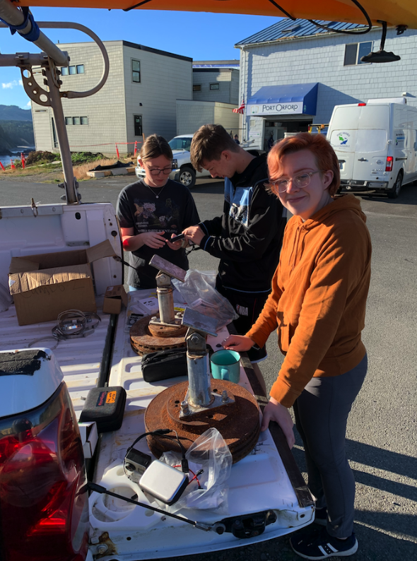
Figure 1: Team prepping CamDo setup for deployment
In the past, I have learned to troubleshoot computer software and lab equipment. However, there were already protocols in place, and my research contributions were part of another student’s pre-defined project. Unlike my previous research experience, for my REU project, I had to learn how to use unfamiliar software, set achievable goals, overcome obstacles, and devise a plan to accomplish them without relying on a team of peers. This is a project Allison and I have been working on together outside of field work, but we have not been without support. Both Victoria Hermanson, a Biological Science Aid with the Antarctic Ecosystem Research Division, and Suzie Winquist, a graduate student at the Marine Mammal Institute, have inspired and guided us through using VIAME for our research questions.
Taking that leap into uncharted waters, we chose to work with two software programs that were new to me called VIAME (Video and Image Analytics for the Marine Environment) and ImageJ. Our goal was to utilize VIAME so that it could distinguish between zooplankton or predators in our CamDo videos (from the hundreds of unannotated frames) and then use ImageJ to quantify the density of zooplankton in those identified frames. Although it has been exciting to use this software that uses Artificial Intelligence (AI) to track and detect prey and predator interactions in video footage, we have encountered many challenges along the way. Within 10 weeks, we had to learn this new software, train it to identify zooplankton and predators, and calculate density using classified frames that we would train. When tackling such an ambitious project in a limited time frame, we expected some setbacks, and through the advice of experienced professionals and the support of Allison (as well as a healthy dose of self-determination), we were able to gain success by breaking down the project into smaller tasks and using trial and error to fix any issues that arose.
Figure 2: Photo of Allison and myself working together to problem solve a VIAME error
Although we have had some failures along the way, we have accomplished a lot, and I am eager to share some results with you. First, we developed and fine-tuned a workflow in VIAME to use AI to identify zooplankton prey and predators in our CamDo videos.
Figure 3: Screenshot of VIAME program that illustrates how we trained a model to identify zooplankton prey (yellow boxes) and fish predators (blue box) in the CamDo videos.
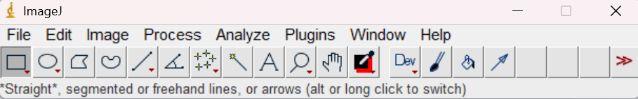
In addition, we implemented a workflow in ImageJ (another software program designed to process and analyze scientific images) to quantify zooplankton density from frames identified by VIAME with zooplankton. Even though it took a lot of trial and error, our primary objectives were met, and we learned a great deal for future GEMM projects.
Figure 4: An example processed output image depicting how ImageJ recognized bodies of zooplankton (black outlines) and counted individual zooplankton ( red dots).
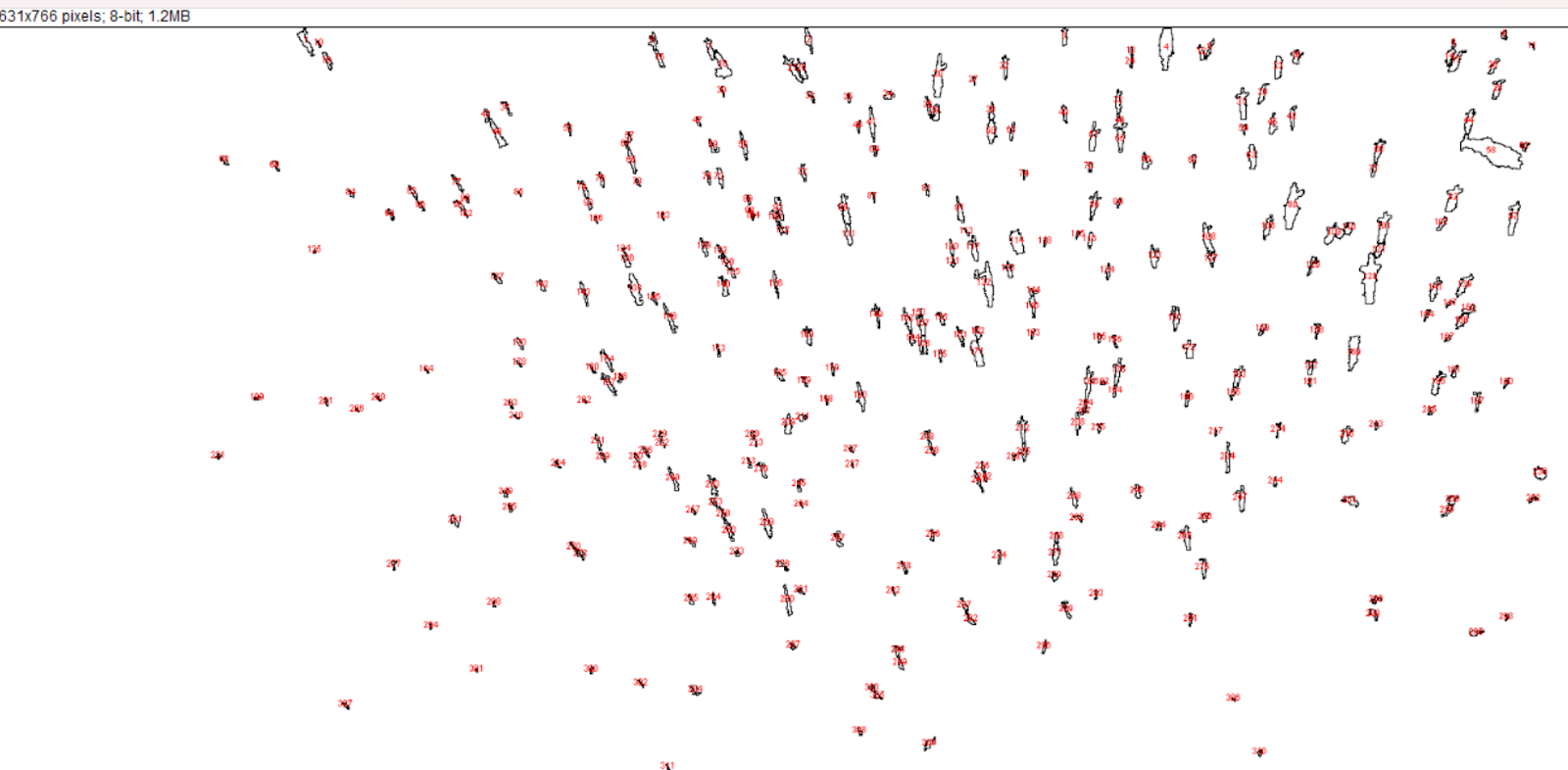
While working on my independent project, I learned that an ability to troubleshoot software and data processing can apply to tricky field work situations as well. For instance, when we lost a weighted cage attachment that protects our RBR concerto sensor, we needed a temporary solution until the divers recovered our lost gear. So our team discussed a few different DIY options. After a frantic afternoon of trial and error, we ultimately decided on using a milk jug as a temporary cage. While it wasn’t the most glamorous solution, the GEMM lab is known to think outside the box as a fundamental part of both the fieldwork and research process.
Figure 5: Photo of Allison testing out our RBR milk jug temporary setup
I have found through this experience that sometimes it is more valuable to struggle and learn skills than to immediately succeed. I am hopeful that this lesson has prepared me for my future, and I couldn’t be more grateful. It has been an interesting summer for me as far as adapting to failures and embracing them. It was a difficult transition leaving my new friends at Hatfield in Newport where I spent my first 4 weeks and embracing an entirely different living dynamic here in Port Orford. With the field season and my research approaching its end, I realize how much I appreciate all the new people I have met here. Before this summer, I had not had many opportunities to interact with similar and enthusiastic marine scientists. Now I live and work with marine science mentors and peers in the field every day, which has been an invaluable experience, and I am grateful for the opportunity to learn from and interact with these inspiring people. It has been a meaningful summer, and I look forward to continuing to build relationships and learn from my failures during this next phase of my life.
Figure 6: Photo of Zoop Troop, from left to right Natalee, Autumn, Allison, Jonah, Aly
Did you enjoy this blog? Want to learn more about marine life, research, and conservation? Subscribe to our blog and get a weekly message when we post a new blog. Just add your name and email into the subscribe box below.
By Jonah Lewis, rising junior at Pacific High School, GEMM Lab Intern 2023
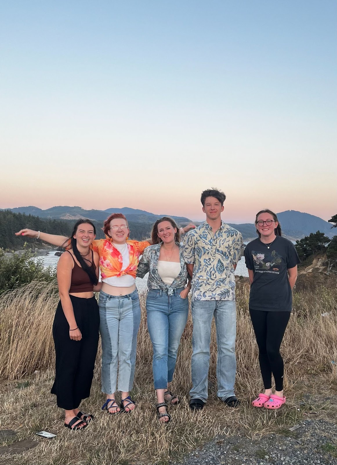
Hello, I’m Jonah Lewis, the other high school intern for the TOPAZ/JASPER Project. I am a rising junior for Pacific High School in Port Orford. I am interested in many things, including computer sciences, electrical sciences, different types of engineering, and lately, marine biology. At the end of February, my biology teacher, Hilary Johnson, was looking for high schoolers to join this internship and I decided that it could be a great experience for me. I applied, and somewhere in March, before I knew it, I was being interviewed by Allison Dawn, our Zoop Troop Sergeant, and Leigh Torres, the head of the operation. I was so nervous for my interview, and tried my best to do well. Then on March 31st, I saw the job offer email, and my family and I were overjoyed. Now that we are in our fourth week, I can say the people and the experiences have been amazing, but my favorite part of all has been the cliff site and the adrenaline rush of tracking a whale moving across the ocean.
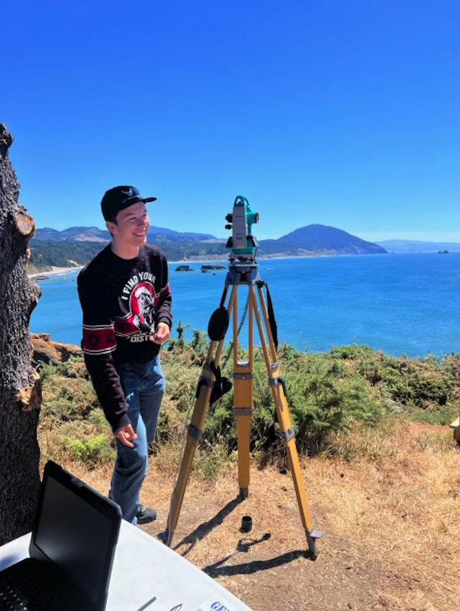
Figure 1: Jonah smiles after fixing a whale using the theodolite.
Theodolite is an important aspect of this research project. This instrument was invented by Leonard Digges back in the 1550’s and is a highly accurate instrument for mapping, engineering, etc. Read here to learn more about the theodolite’s component parts, written by last year’s intern Nichola Gregory, a previous JASPER intern. In Port Orford, we use it for tracking where a gray whale blows and surfaces! Setting up the theodolite can be a challenge for newcomers, but as you repeatedly put this device together, and then take it down, you understand and can troubleshoot better and faster than the previous time. It took me and the team some practice to be able to get all three ways it needs to level just right, or else the instrument decides to throw a fit. For example, when the theodolite isn’t exactly leveled right, or maybe the batteries are low, or the cord just isn’t plugged in all the way, it will just beep at you, trying to say there is an error. After the theodolite is properly leveled, you connect it to the computer that runs our software program called Pythagoras.
Not only does the physical setup require care, but “fixing” a whale requires technique. Here, we are trained to be both accurate and precise when following our focal species. To be accurate, we would need to position the theodolite scope so that the whale is close to the crosshairs. To be precise, we need to fix the whale in the same location on the theodolite crosshairs consistently. Our team has learned how to be both accurate and precise.
Figure 2: Accurate and precise diagram using the crosshairs of a theodolite as reference, diagram by A. Dawn.
Being on cliff team can get tedious, even when you are not using the theodolite to fix a whale. Staring at the waves and the horizon can feel like an eternity, especially when gray whales aren’t active in our study area. Yet, during this time we have to be “on effort”. Being on effort is making sure you scan the horizon consistently, both you and a partner are constantly looking at our study sites. All this is best represented by our team manager Allison: On the cliff with her, she is always looking at the ocean, paying attention to both sites, and for at least the first hour or longer, she will not sit down.
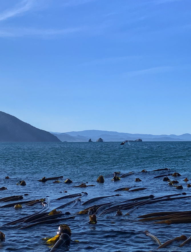
Figure 3: Kelp bed behind the jetty while a whale flukes in the background.
After we collect all of our data from kayak and cliff each day, we head down to the dry lab and get prepared to download and transfer our data to a hard drive known as “Tharp”. I learned that Marie Tharp was a woman in the 20th century, who mapped the ocean floors, which helps scientists even now. (The GEMM Lab names each hard drive after famous scientists; it helps to track the many hard drives.) When I use the hard drive, I think about her and about how I also helped collect data for mapping features in our marine study site. During the first week of data collection, Allison and I looked through the theodolite scope, found obvious kelp patches on the surface of the water, and fixed many times around the edges, making a complete polygon around the kelp beds.
Figure 4: Team bonding at the Prehistoric Gardens in Port Orford
This internship for the past four weeks has been an amazing experience. In addition to our fieldwork, I’ve been able to participate and connect with many other interns and professionals here at the Field Station. I have also enjoyed connecting with visitors from all different areas who come by and ask what research we’re doing on the cliff. At the field station I have fun hanging with the guys at the house as well, where we play sports in our downtime and cook together. I also learn about what projects they are doing, from urchin culling to sea otter research, it all fascinates me. I have helped POSS (Port Orford Sustainable Seafood) with bagging fish, washing dishes, and in return they provide samples of the amazing food they make. I am overjoyed about what I have learned and the people I have met during this experience, and am so thankful to be a part of the ninth year of this project.
Did you enjoy this blog? Want to learn more about marine life, research and conservation? Subscribe to our blog and get weekly updates and more! Just add your name into the subscribe box below!
By Natalee Webster, Oregon State University rising senior, GEMM Lab Intern 2023
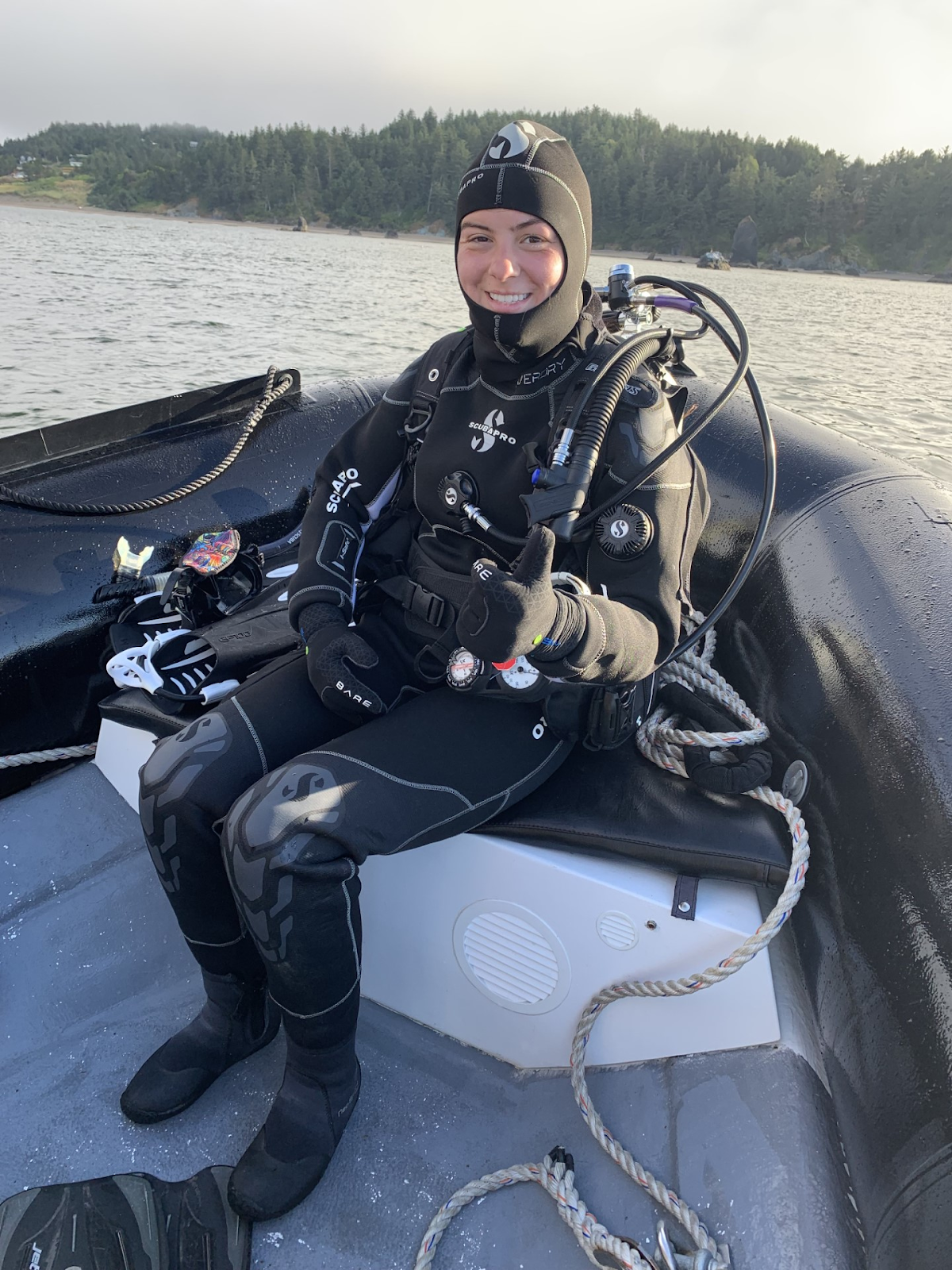
When I was younger, I was terrified of the water, sobbing on a rock across the river, afraid to be immersed in the unknown. Flash-forward to the present and I have one more year left to finish my undergraduate degree in Biology at Oregon State University with a focus in Marine Biology. I was a little hesitant about choosing a more focused degree since I wasn’t sure what aspect of sciences piqued my interest more. However my curiosity for the ocean grew as I took the PADI Open Water scuba class through school. After earning my certification, I discovered I loved being in the water, and seeing the habitats I read about firsthand. I quickly took my Advanced Scuba and worked my way up to Divemaster, and ultimately AAUS Scientific diving. This new certification provided me with skills for a career in marine biology, performing tasks and taking surveys underwater. Through the diving community at OSU, I met Allison Dawn, our graduate student leader of the TOPAZ/JASPER project studying gray whale foraging ecology. Through meeting her I was informed about this project and decided to apply. Now, as I write, we are working on week three of this project, and I could not be happier with my decision. This internship has already taught me so much about the hard work and logistics that goes into studying the behaviors of large marine mammals in the field, as well as what it is like to closely work with a team to accomplish our goals.
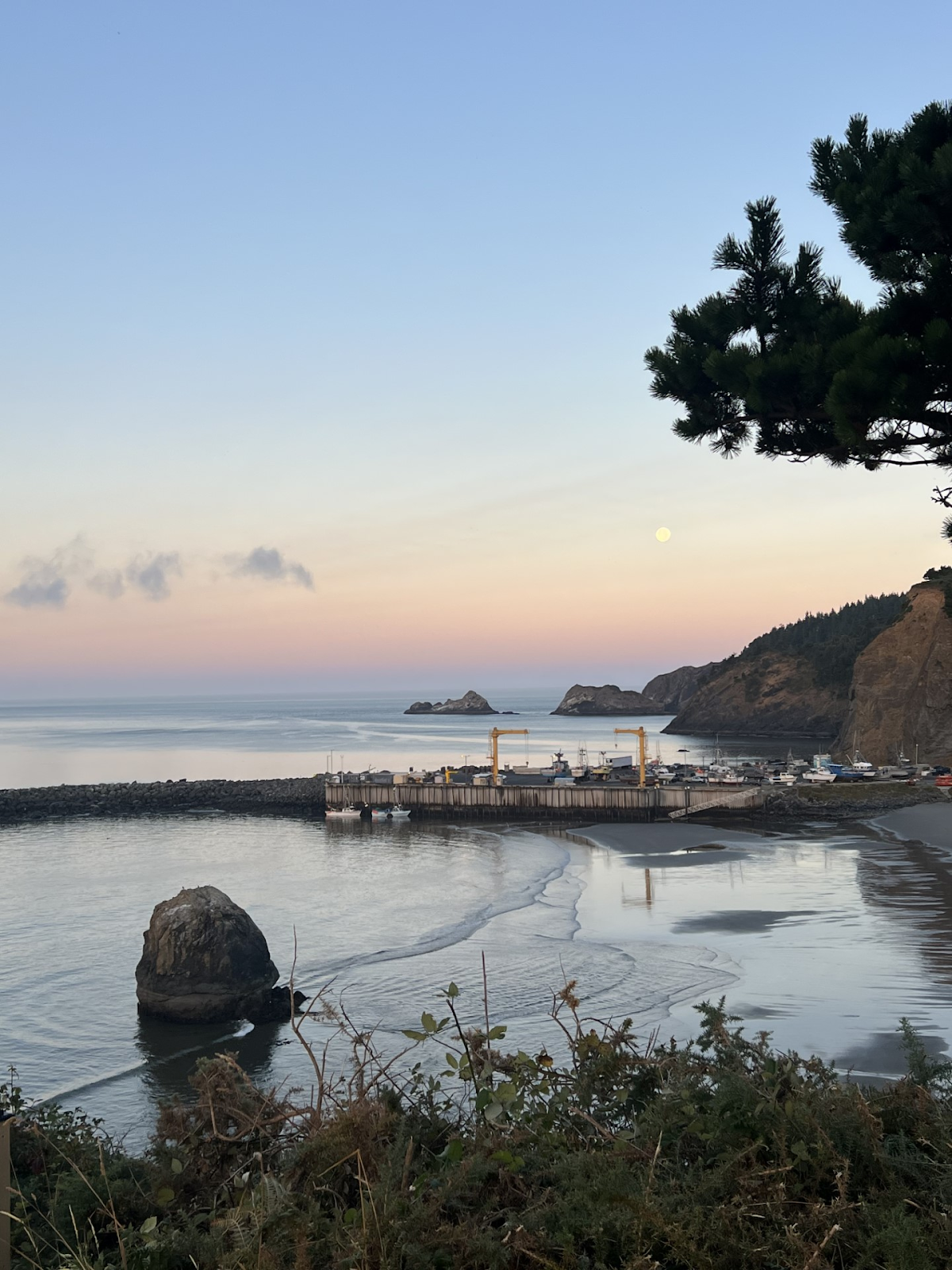
Figure 1. Port of Port Orford at dawn.
Each morning we wake up before the sun with a new set of goals, with a variety of tasks ahead that certainly keeps you on your toes. Long-time readers will know of our kayak and cliff methods, but another aspect of this project is our CamDo underwater cameras. These are cameras that we place in Mill Rocks and Tichenor Cove, our two sampling sites, for a week at a time for longer term footage. In order to deploy these cameras we utilize scuba equipment to properly place them in a location. When the week is up, we go to recover the cameras to gather the data, replace SD card and batteries, and reset them for another week of underwater video footage.
Although CamDo deployment is not a required part of this internship, I have been able to use my scientific diving certification to assist this project on the dives. I appreciate the opportunity to take apply skills to assist the project from a different perspective. Before my first week here I had never dove off the Oregon coast from a boat, so this task was daunting, as I was still getting to know everyone around the field station, and get a sense of my environment.
Figure 2. Photo of Natalee geared up for a dive in Mill Rocks.
Our very first dive at Mill Rocks was intimidating but exciting. Allison and I got up before dawn to prepare the cameras and get to the dive boat the Black Pearl. Allison is our dive tender, handling equipment and logistics, and we worked alongside two other divers — Caroline Rice, an intern with ORKA here at the Port Orford field station, and Kevin Buch, our dive leader and the dive safety officer and scientific diving professor at OSU. Once we rolled off the boat and started our descent I began to feel more in my element as the green waters surrounded us. As we continued further and further to the ocean floor, I realized that visibility was turning from a green you could see rays of sunlight through, into a dark black — barely visible further than five inches from my face. We were able to position the camera lander as needed, but we could not secure the camera because of those black-out conditions. While I waited in the waters for direction on the dive, I put my face as close to the rock as the tides would let me and I saw a purple urchin underwater for the first time, and let me tell you, in the dark waters it was eerie. We finally surfaced and got on the boat to venture off to Tichenor Cove in an attempt to deploy the other CAMDO. Here, I realized that despite the best preparation, scientists need to remain adaptable and determined in the face of challenging ocean conditions.
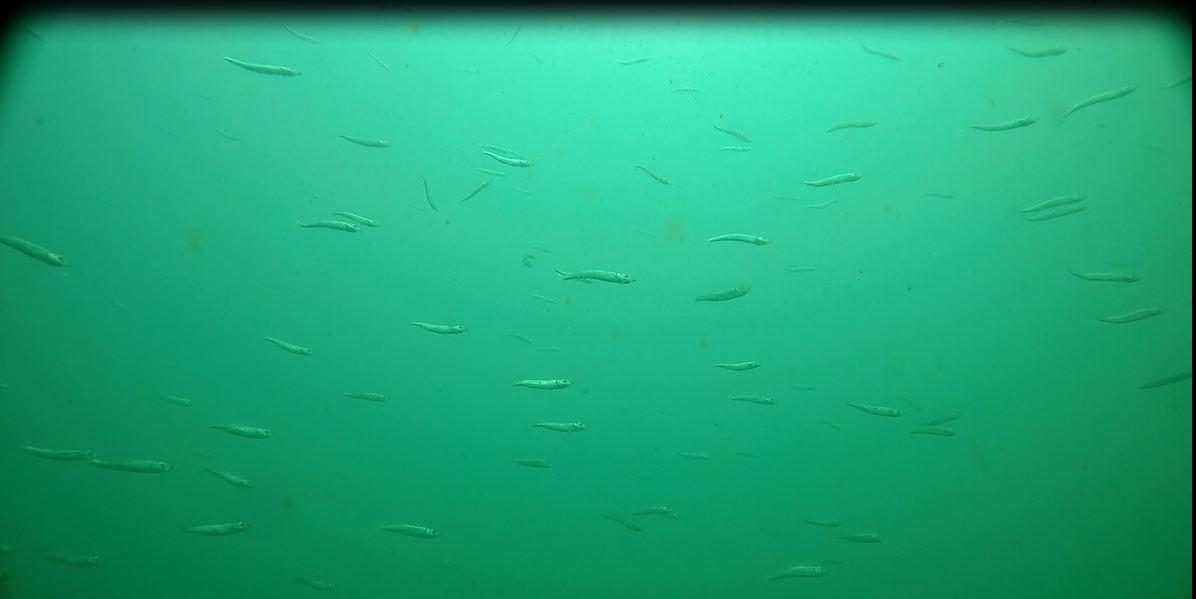
Figure 3. A screenshot of CAMDO footage showing fish swimming in the water column.
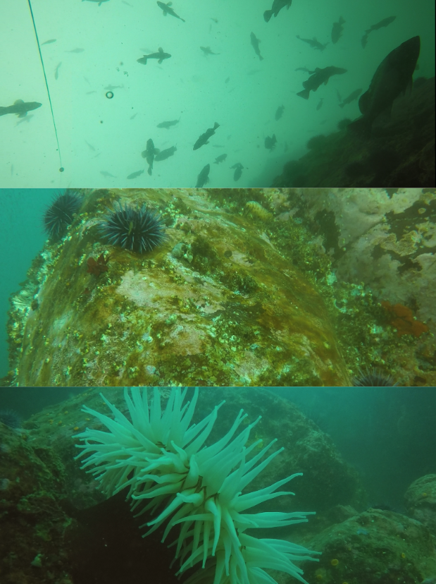
As we prepared for the next dive and began our descent, I silently wondered what I had gotten myself into. I hoped that not all dives off the Oregon Coast were as dark. While slowly descending into Tichenor Cove, I was pleasantly surprised to see that the waters were beautiful in contrast to the darkness of Mill Rocks. Tichenor seemed to be a safe haven in comparison to Mill Rocks; rather than the strong current pushing me along the rocks and urchins, I was able to calmly swim through the rocks and look at the many sea stars, nudibranch, anemones, and different hues of purple urchins living along them.
Figure 4. Photos taken from GoPro of Tichenor Cove environment, showing rockfish, urchins, and an anemone.
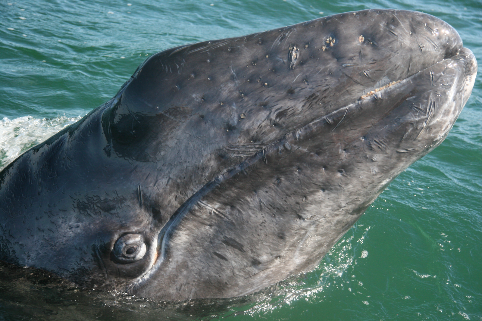
More recently, we recovered the camera for data processing. While comparing the footage between the two locations, I have learned the ocean is incredibly variable. From clear blue waters where you can clearly see juvenile and adult fish swimming in the water column, compared to nothing but murky brown and black waters. This variability inspired me to think more deeply about what the gray whales see while they forage for food. Dr. Leigh Torres visited our team and I was able to discuss our dives and inquire about the methods these whales use in order to eat. My basic knowledge of whale anatomy tells me that they have eyes; however, I was curious if they used eyesight to locate zooplankton and other food. Leigh informed me that these whales have whiskers! This was an exciting discovery for me, I googled it later and found that gray whales and many other baleen whales have hair follicles, called vibrissae (watch this NOAA video to learn more!), around their rostrum and mouth they use as tactile sensors. Leigh Torres has hypothesized a “sense-of-scale” that illustrates an interchange of sensory modalities such as vision, audition, chemoreception, magnetoreception and somatosensory perception that allows whales to track and capture of prey (Torres 2017). Research in this sensory field continues to grow to better understand how marine mammals capture and track prey at various scales.
Figure 5. Image of a gray whale, the spot markings along its jaw and rostrum are hair follicles known as vibrissae. (2016)
Seeing these small segments of their habitat myself while underwater has given me much more respect for how these gray whales are able to forage in such a challenging and changing environment. My teammate Autumn is currently working on quantifying the zooplankton abundance recorded in the footage taken through CAMDO, so stay tuned on the Port Orford blogs to hear more about their project!
Figure 6. Photo of Aly, Natalee, and Autumn before kayak training. Honorable mention to the bucket hats.
The opportunity to participate in this year’s Gray Whale Foraging Ecology project is something I will not take for granted and will appreciate greatly for years. It has given me the opportunity to grow my knowledge about the marine environment that I have been fascinated with, as well as given me skills and training in methods of field research. I even got to apply my hard-earned underwater skills and conduct my first official scientific dives! I have been able to interact with the long-time locals of Port Orford, whether it be a fisherman sharing their orca encounter tales to retired photographers that chase the whales along the shore. The field station houses many projects focusing on different aspects of the Oregon coast from sea urchins and kelp to river otters along the shores and to outreach programs within the community. When everyone is settling back into the field station after their long day of work, it is great to be gathered in the kitchen and hear about the progress we’ve made and the experiences we’ve had. I look forward to the remaining three weeks I have in Port Orford with this community and my team! Wish us luck as we prepare to deploy the next round of CamDo cameras next week.
Did you enjoy this blog? Want to learn more about marine life, research and conservation? Subscribe to our blog and get weekly updates and more! Just add your name into the subscribe box below!
References
Torres, L.G. (2017), A sense of scale: Foraging cetaceans’ use of scale-dependent multimodal sensory systems. Mar Mam Sci, 33: 1170-1193. https://doi.org/10.1111/mms.12426