Oregon Coast – Page 6 – Geospatial Ecology of Marine Megafauna Laboratory

The impact of science

By Lisa Hildebrand, MSc student, OSU Department of Fisheries & Wildlife, Marine Mammal Institute, Geospatial Ecology of Marine Megafauna Lab

What do I mean by impact? There are different ways to measure the impact of science and I bet that the readers of this blog had different ideas pop into their heads when they read the title. My guess is that most ideas were related to the impact factor (IF) of a journal, which acts as a measure of a journal’s impact within its discipline and allows journals to be compared. Recent GEMM Lab graduate and newly minted Dr. Leila Lemos wrote a blog about this topic and I suggest reading it for more detail. In a nutshell though, the higher the IF, the more prestigious and impactful the journal. It is unsurprising that scientists found a way to measure our impact on the broader scientific community quantitatively.

However, IFs are not the impact I was referring to in my title. The impact I am talking about is arguably much harder to measure because you can’t easily put a number on it. I am talking about the impact we have on communities and individuals through outreach and engagement. The GEMM Lab’s Port Orford gray whale ecology project, which I lead, is going into its 6^th consecutive year of summer field work this year. Outreach and engagement are two core components of the project that I have become very invested in since I started in 2018. And so, since we are only one week away from the field season commencing (yes, somehow it’s mid-July already…), for this week’s blog I have decided to reflect on what scientific outreach and engagement is, how we have tried to do both in Port Orford, and some of the associated highs and lows.

2018 team member Dylan presenting at the Port Orford community presentation. Source: T. Calvanese.

I think almost everyone in the scientific community would agree that outreach and engagement are important and that we should strive to interact frequently with the public to be transparent and build public trust, as well as to enable mutual learning. However, in my opinion, most scientists rarely put in the work needed to actually reach out to, and engage with, the community. Outreach and engagement have become buzzwords that are often thrown around, and with some hand-waving, can create the illusion that scientists are doing solid outreach and engagement work. For some, the words are probably even used interchangeably, which isn’t correct as they mean two different things.

Outreach and engagement should be thought of as occurring on two different ends of a spectrum. Outreach occurs in a one-way direction. Examples of outreach are public seminars delivered by a scientist (like Hatfield’s monthly Science on Tap) or fairs where the public is invited to come and talk to different scientific entities at their respective booths (like Hatfield’s annual Marine Science Day). Outreach is a way for scientists to disseminate their research to the public and often do not warrant the umbrella term engagement, as these “conversations” are not two-way. Engagement is collaborative and refers to intentional interactions where both sides (public and scientist) share and receive. It goes beyond a scientist telling the public about what they have been doing, but also requires the scientist to listen, absorb, and implement what the views from the ‘other side’ are.

2015 team tracking a whale on Graveyard Point above the port of Port Orford. Source: F. Sullivan.

Now that I have (hopefully) clarified the distinction between the two terms, I am going to shift the focus to specifically talk about the Port Orford project. Before I do, I would like to emphasize that I do not think our outreach and engagement is the be-all and end-all. There is definitely room for improvement and growth, but I do believe that we actively work hard to do both and to center these aspects within the project, rather than doing it as an afterthought to tick a box.

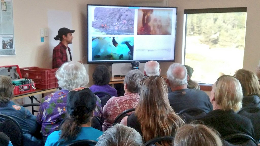
In talking about outreach and engagement, I have been using the words ‘public’ and ‘community’. I think these words conjure an image of a big group of people, an entire town, county, state or even nation. While this can be the case, it can also refer to smaller groups of people, even individuals. The outreach we conduct for the Port Orford project certainly occurs at the town-level. At the end of every field season, we give a community presentation where the field team and Leigh present new findings and give a recount of the field season. In the past, various teams have also given talks at the Humbug Mountain Campground and at Redfish Rocks Community Team events. These events, especially the community presentation, have been packed to the brim every year, which shows the community’s interest for the gray whales and our research. In fact, Tom Calvanese, the OSU Port Orford Field Station manager, has shared with me that now in early summer, Port Orford residents ask him when the ‘whale team’ is returning. I believe that our project has perhaps shifted the perception the local community has of scientists a little bit. Although in our first year or two of the project we may have been viewed as nosy outsiders, I feel that now we are almost honorary members within the community.

A packed room at the 2017 Port Orford community presentation. Photo: GEMM Lab.

Our outreach is not just isolated to one or two public talks per field season though. We have been close collaborators with South Coast Tours (SCT), an adventure tour company headed by Dave Lacey, since the start of the project. During the summer, SCT has almost daily kayak and fishing tours (this year, boat tours too!) out of Port Orford. The paddle routes of SCT and our kayak team will typically intersect in Tichenor’s Cove around mid-morning. When this happens, we form a little kayak fleet with the tour and research kayaks and our kayak team gives a short, informal talk about our research. We often pass around samples of zooplankton we just collected and answer questions that many of the paddlers have. These casual interactions are a highlight to the guests on SCT’s tours (Dave’s words, not mine) and they also provide an opportunity for the project’s interns to practice their science communication skills in a ‘low-stakes’ setting.

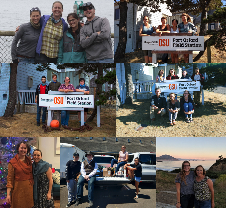
The nature of our engagement is more at the individual-level. Since the project’s conception in 2015, the team has been composed of some combination of 4-5 students, be it high school, undergraduate or graduate students. Aside from Florence Sullivan and myself as the GEMM Lab graduate student project leads, in total, we have had 16 students participate in the program, of which 4 were high school students (two from Port Orford’s Pacific High School and two from Astoria High School), 11 OSU and Lawrence University undergraduates, and 1 Duke University graduate student. This year we will be adding 3 more to the total tally (1 Pacific High School student, 1 OSU undergrad, and 1 graduate student from the Vrije Universiteit Brussel in Belgium). I am the first to admit that our yearly (and total) numbers of ‘impacted’ students is small. Limitations of funding and also general logistics of coordinating a large group of interns to participate in field work prevent us from having a larger cohort participate in the field season every summer. However, the impact on each of these students is huge.

The 2019 team with Dave Lacey who instructed our kayak paddle & safety course. Photo: L. Hildebrand.

If I had to pick one word to describe the 6-week Port Orford field season, it would be ‘intense’. The word is perfect because it can simultaneously describe something positive and negative, and the Port Orford field season definitely has elements of both. Both as a team and as individuals we experience incredible high points (an example being last year when we saw Port Orford’s favorite whale ‘Buttons’ breach multiple times on several different days), but we also have pretty low points (I’m thinking of a day in 2018 when two of my interns tried incredibly hard to get our GoPro stick dislodged from a rocky crevice for over 1-hour before radioing me to tell me they couldn’t retrieve it). These highs and lows occur on top of the team’s slowly depleting levels of energy as the field season goes on; with every day we get up at 5:30 am and we get a little more exhausted. The work requires a lot of brain power, a lot of muscle, and a lot of teamwork. Like I said, it’s intense and that’s coming from someone who had several years of marine mammal field work experience before running this project for the first time in 2018. The majority of the interns who have participated in our project have had no marine mammal field experience, some have had no field experience at all. It’s double, if not triple, intense for the interns!

I ask a lot of my interns. I am aware of that. It has been a steep learning curve for me since I took on the project in 2018. I’ve had to adjust my expectations and remember not to measure the performance of my interns against my own. I can always give 110% during the field season, even when I’m exhausted, because the stakes are high for me. After all, the data that is being collected feeds straight into my thesis. However, it took me a while to realize that the stakes, and therefore the motivation, aren’t the same for my interns as they are for me. And so, expecting them to perform at the same level I am, is unfair. I believe I have grown a lot since running that first field season. I have taken the feedback from interns to heart and tried to make adjustments accordingly. While those adjustments were hard because it ultimately meant making compromises that affected the amount of data collected, I recognize and respect the need to make those adjustments. I am incredibly grateful to all of the interns, including the ones that participated before my leadership of the project, who really gave it their all to collect the data that I now get to dig into and draw conclusions from.

2016 interns Kelli and Catherine paddling to a kayak sampling station. Photo: F. Sullivan.

But, as I said before, engagement is not one-sided, and I am not the only one who benefits from having interns participate in the project. The interns themselves learn a wealth of skills that are valuable for the future. Some of these skills are very STEM (Science, Technology, Engineering & Mathematics) specific (e.g. identifying zooplankton with a microscope, tracking whales with a theodolite), but a lot of them are transferrable to non-STEM futures (e.g. attention to detail and concentration required for identifying zooplankton, team work, effective communication). Our reach may be small with this project but the impact that participating in our internship has on each intern is a big one. Three of our four high school interns have gone on to start college. One plans to major in Marine Studies (in part a result of participating in this internship) while another decided to go to college to study Biology because of this internship. Several of the undergraduate students that participated in the 2015, 2016, 2017 & 2018 field seasons have gone on to start Master’s degrees at graduate schools around the country (3 of which have already graduated from their programs). A 2015 intern now teaches middle school in Washington and a 2016 intern is working with Oceans Initiative on their southern resident killer whale project this summer. Leigh, Florence and I have written many letters of recommendations for our interns, and these letters were not written out of duty, but out of conviction.

I love working closely with students and watching them grow. For the last two years, my proudest moment has always been watching my interns present our research at the annual community presentation we give at the end of the field season in Port Orford. No matter the amount of lows and struggles I experienced throughout the season, I watch my interns and my face almost hurts because of the huge smile on my face. The interns truly undergo a transformation where at the start of the season they are shy or feel inadequate and awkward when talking to the public about gray whales and the methods we employ to study them. But on that final day, there is so much confidence and eloquence with which the interns talk about their internship, that they are oftentimes even comfortable enough to crack jokes and share personal stories with the audience. As I said before, engagement of this nature is hard to measure and put a number on. Our statistic (engaging with 16 students) makes it sound like a small impact, but when you dig into what these engagements have meant for each student, the impact is enormous.

All of the past PO gray whale ecology teams, from left to right: 2015 (Sarah, Florence, Cricket, Justin), 2016 (Florence, Kelli, Catherine, Cathryn), 2017 (Nathan, Quince, Florence, Morgan), 2018 (Haley, Robyn, Hayleigh, Dylan, Lisa), and 2019 (Anthony, Donovan, Lisa, Mia). Bottom left: Florence and Leigh; bottom right: Lisa and Leigh.

I treasure my 6 weeks in Port Orford. Even though they are intense and there are new challenges every year, they bring me a lot of happiness. And it’s only in part because I get to see gray whales and kayak on an (almost) daily basis. A large part is because of the bonds I have formed and continue to cultivate with Port Orford locals, the leaps and bounds I know the interns will make, and the fact that the gray whales, completely unknowingly, bring together a small group of students and a community every year.

If you feel like taking a trip down memory lane, below are the links of the blogs written by previous PO interns:

2015: Cricket, Justin, Sarah

2016: Catherine, Kelli, Cathryn

2017: Morgan, Nathan, Quince

2018: Haley, Dylan, Hayleigh, Robyn

2019: Mia, Donovan, Anthony

You can’t build a pyramid without the base: diving into the foundations of behavioral ecology to understand cetacean foraging

By Lisa Hildebrand, MSc student, OSU Department of Fisheries & Wildlife, Marine Mammal Institute, Geospatial Ecology of Marine Megafauna Lab

The last two months have been challenging for everyone across the world. While I have also experienced lows and disappointments during this time, I always try to see the positives and to appreciate the good things every day, even if they are small. One thing that I have been extremely grateful and excited about every week is when the clock strikes 9:58 am every Thursday. At that time, I click a Zoom link and after a few seconds of waiting, I am greeted by the smiling faces of the GEMM Lab. This spring term, our Principal Investigator Dr. Leigh Torres is teaching a reading and conference class entitled ‘Cetacean Behavioral Ecology’. Every week there are 2-3 readings (a mix of book chapters and scientific papers) focused on a particular aspect of behavioral ecology in cetaceans. During the first week we took a deep dive into the foundations of behavioral ecology (much of which is terrestrial-based) and we have now transitioned into applying the theories to more cetacean-centric literature, with a different branch of behavior and ecology addressed each week.

Leigh dedicated four weeks of the class to discussing foraging behavior, which is particularly relevant (and exciting) to me since my Master’s thesis focuses on the fine-scale foraging ecology of gray whales. Trying to understand the foraging behavior of cetaceans is not an easy feat since there are so many variables that influence the decisions made by an individual on where and when to forage, and what to forage on. While we can attempt to measure these variables (e.g., prey, environment, disturbance, competition, an individual’s health), it is almost impossible to quantify all of them at the same time while also tracking the behavior of the individual of interest. Time, money, and unworkable weather conditions are the typical culprits of making such work difficult. However, on top of these barriers is the added complication of scale. We still know so little about the scales at which cetaceans operate on, or, more importantly, the scales at which the aforementioned variables have an effect on and drive the behavior of cetaceans. For instance, does it matter if a predator is 10 km away, or just when it is 1 km away? Is a whale able to sense a patch of prey 100 m away, or just 10 m away? The same questions can be asked in terms of temporal scale too.

*What is that gray whale doing in the kelp? Source: F. Sullivan.*

As such, cetacean field work will always involve some compromise in data collection between these factors. A project might address cetacean movements across large swaths of the ocean (e.g., the entire U.S. west coast) to locate foraging hotspots, but it would be logistically complicated to simultaneously collect data on prey distribution and abundance, disturbance and competitors across this same scale at the same time. Alternatively, a project could focus on a small, fixed area, making simultaneous measurements of multiple variables more feasible, but this means that only individuals using the study area are studied. My field work in Port Orford falls into the latter category. The project is unique in that we have high-resolution data on prey (zooplankton) and predators (gray whales), and that these datasets have high spatial and temporal overlap (collected at nearly the same time and place). However, once a whale leaves the study area, I do not know where it goes and what it does once it leaves. As I said, it is a game of compromises and trade-offs.

Ironically, the species and systems that we study also live a life of compromises and trade-offs. In one of this week’s readings, Mridula Srinivasan very eloquently starts her chapter entitled ‘Predator/Prey Decisions and the Ecology of Fear’ in Bernd Würsig’s ‘Ethology and Behavioral Ecology of Odontocetes’ with the following two sentences: “Animal behaviors are governed by the intrinsic need to survive and reproduce. Even when sophisticated predators and prey are involved, these tenets of behavioral ecology hold.”. Every day, animals must walk the tightrope of finding and consuming enough food to survive and ensure a level of fitness required to reproduce, while concurrently making sure that they do not fall prey to a predator themselves. Krebs & Davies (2012) very ingeniously use the idea of economic analysis of costs and benefits to understand foraging behavior (but also behavior in general). While foraging, individuals not only have to assess potential risk (Fig. 1) but also decide whether a certain prey patch or item is profitable enough to invest energy into obtaining it (Fig. 2).

Leigh’s class has been great, not only to learn about foundational theories but to then also apply them to each of our study species and systems. It has been exciting to construct hypotheses based on the readings and then dissect them as a group. As an example, Sih’s 1984 paper on the behavioral response race of predators and prey prompted a discussion on responses of predators and prey to one another and how this affects their spatial distributions. Sih posits that since predators target areas with high prey densities, and prey will therefore avoid areas that predators frequent, their responses are in conflict with one another. Resultantly, there will be different outcomes depending on whichever response dominates. If the predator’s response dominates (i.e. predators are able to seek out areas of high prey density before prey can respond), then predators and prey will have positively correlated spatial distributions. However, if the prey responses dominate, then the spatial distributions of the two should be negatively correlated, as predators will essentially always be ‘one step behind’ the prey. Movement is most often the determinant factor to describe the strength of these relationships.

Video 1. Zooplankton closest to the camera will jump or dart away from it. Source: GEMM Lab.

So, let us think about this for gray whales and their zooplankton prey. The latter are relatively immobile. Even though they dart around in the water column (I have seen them ‘jump’ away from the GoPro when we lower it from the kayak on several occasions; Video 1), they do not have the ability to maneuver away fast or far enough to evade a gray whale predator moving much faster. As such, the predator response will most likely always be the strongest since gray whales operate at a scale that is several orders of magnitude greater than the zooplankton. However, the zooplankton may not be as helpless as I have made them seem. Based on our field observations, it seems that zooplankton often aggregate beneath or around kelp. This behavior could potentially be an attempt to evade predators as the kelp and reef crevices may serve as a refuge. So, in areas with a lot of refuges, the prey response may in fact dominate the relationship between gray whales and zooplankton. This example demonstrates the importance of habitat in shaping predator-prey interactions and behavior. However, we have often observed gray whales perform “bubble blasts” in or near kelp (Video 2). We hypothesize that this behavior could be a foraging tactic to tip the see-saw of predator-prey response strength back into their favor. If this is the case, then I would imagine that gray whales must decide whether the energetic benefit of eating zooplankton hidden in kelp refuges outweighs the energy required to pursue them (Fig. 2). On top of all these choices, are the potential risks and threats of boat traffic, fishing gear, noise, and potential killer whale predation (Fig. 1). Bringing us back to the analogy of economic analysis of costs and benefits to predator-prey relationships. I never realized it so clearly before, but gray whales sure do have a lot of decisions to make in a day!

Video 2. Drone footage of a gray whale foraging in kelp and performing a “bubble blast” at 00:40. Footage captured under NMFS permit #21678. Source: GEMM Lab.

Trying to tease apart these nuanced dynamics is not easy when I am unable to simply ask my study subjects (gray whales) why they decided to abandon a patch of zooplankton (Were the zooplankton too hard to obtain because they sought refuge in kelp, or was the patch unprofitable because there were too few or the wrong kind of zooplankton?). Or, why do gray whales in Oregon risk foraging in such nearshore coastal reefs where there is high boat traffic (Does their need for food near the reefs outweigh this risk, or do they not perceive the boats as a risk?). So, instead, we must set up specific hypotheses and use these to construct a thought-out and informed study design to best answer our questions (Mann 2000). For the past few weeks, I have spent a lot of time familiarizing myself with spatial packages and functions in R to start investigating the relationships between zooplankton and kelp hidden in the data we have collected over 4 years, to ultimately relate these patterns to gray whale foraging. I still have a long and steep journey before I reach the peak but once I do, I hope to have answers to some of the questions that the Cetacean Behavioral Ecology class has inspired.

Literature cited

Krebs, J. R., and N. B. Davies. 2012. Economic decisions and the individual in Davies, N. B. et al., eds. An introduction to behavioral ecology. John Wiley & Sons, Oxford.

Mann, J. 2000. Unraveling the dynamics of social life: long-term studies and observational methods in Mann, J., ed. Cetacean societies: field studies of dolphins and whales. University of Chicago Press, Chicago.

Sih, A. 1984. The behavioral response race between predator and prey. The American Naturalist 123:143-150.

Srinivasan, M. 2019. Predator/prey decisions and the ecology of fear in Würsig, B., ed. Ethology and ecology of odontocetes. Springer Nature, Switzerland.

Can sea otters help kelp under a changing climate?

By Dominique Kone¹ and Sara Hamilton²

¹Masters Student in Marine Resource Management, ²Doctoral Student in Integrative Biology

Five years ago, the North Pacific Ocean experienced a sudden increase in sea surface temperature (SST), known as the warm blob, which altered marine ecosystem function and structure (Leising et al. 2015). Much research illustrated how the warm blob impacted pelagic ecosystems, with relatively less focused on the nearshore environment. Yet, a new study demonstrated how rising ocean temperatures have partially led to bull kelp loss in northern California. Unfortunately, we are once again observing similar warming trends, representing the second largest marine heatwave over recent decades, and signaling the potential rise of a second warm blob. Taken together, all these findings could forecast future warming-related ecosystem shifts in Oregon, highlighting the need for scientists and managers to consider strategies to prevent future kelp loss, such as reintroducing sea otters.

In northern California, researchers observed a dramatic ecosystem shift from productive bull kelp forests to purple sea urchin barrens. The study, led by Dr. Laura Rogers-Bennett from the University of California, Davis and California Department of Fish and Wildlife, determined that this shift was caused by multiple climatic and biological stressors. Beginning in 2013, sea star populations were decimated by sea star wasting disease (SSWD). Sea stars are a main predator of urchins, causing their absence to release purple urchins from predation pressure. Then, starting in 2014, ocean temperatures spiked with the warm blob. These two events created nutrient-poor conditions, which limited kelp growth and productivity, and allowed purple urchin populations to grow unchecked by predators and increase grazing on bull kelp. The combined effect led to approximately 90% reductions in bull kelp, with a reciprocal 60-fold increase in purple urchins (Figure 1).

Figure 1. Kelp loss and ecosystem shifts in northern California (Rogers-Bennett & Catton 2019).

These changes have wrought economic challenges as well as ecological collapse in Northern California. Bull kelp is important habitat and food source for several species of economic importance including red abalone and red sea urchins (Tegner & Levin 1982). Without bull kelp, red abalone and red sea urchin populations have starved, resulting in the subsequent loss of the recreational red abalone ($44 million) and commercial red sea urchin fisheries in Northern California. With such large kelp reductions, purple urchins are also now in a starved state, evidenced by noticeably smaller gonads (Rogers-Bennett & Catton 2019).

Biogeographically, southern Oregon is very similar to northern California, as both are composed of complex rocky substrates and shorelines, bull kelp canopies, and benthic macroinvertebrates (i.e. sea urchins, abalone, etc.). Because Oregon was also impacted by the 2014-2015 warm blob and SSWD, we might expect to see a similar coastwide kelp forest loss along our southern coastline. The story is more complicated than that, however. For instance, ODFW has found purple urchin barrens where almost no kelp remains in some localized places. The GEMM Lab has video footage of purple urchins climbing up kelp stalks to graze within one of these barrens near Port Orford, OR (Figure 2, left). In her study, Dr. Rogers-Bennett explains that this aggressive sea urchin feeding strategy is potentially a sign of food limitation, where high-density urchin populations create intense resource competition. Conversely, at sites like Lighthouse Reef (~45 km from Port Orford) outside Charleston, OR, OSU and University of Oregon divers are currently seeing flourishing bull kelp forests. Urchins at this reef have fat, rich gonads, which is an indicator of high-quality nutrition (Figure 2, right).

Satellites can detect kelp on the surface of the water, giving scientists a way to track kelp extent over time. Preliminary results from Sara Hamilton’s Ph.D. thesis research finds that while some kelp forests have shrunk in past years, others are currently bigger than ever in the last 35 years. It is not clear what is driving this spatial variability in urchin and kelp populations, nor why southern Oregon has not yet faced the same kind of coastwide kelp forest collapse as northern California. Regardless, it is likely that kelp loss in both northern California and southern Oregon may be triggered and/or exacerbated by rising temperatures.

Figure 2. Left: Purple urchin aggressive grazing near Port Orford, OR (GEMM Lab 2019). Right: Flourishing bull kelp near Charleston, OR (Sara Hamilton 2019).

The reintroduction of sea otters has been proposed as a solution to combat rising urchin populations and bull kelp loss in Oregon. From an ecological perspective, there is some validity to this idea. Sea otters are a voracious urchin predator that routinely reduce urchin populations and alleviate herbivory on kelp (Estes & Palmisano 1974). Such restoration and protection of bull kelp could help prevent red abalone and red sea urchin starvation. Additionally, restoring apex predators and increasing species richness is often linked to increased ecosystem resilience, which is particularly important in the face of global anthropogenic change (Estes et al. 2011)

While sea otters could alleviate grazing pressure on Oregon’s bull kelp, this idea only looks at the issue from a top-down, not bottom-up, perspective. Sea otters require a lot of food (Costa 1978, Reidman & Estes 1990), and what they eat will always be a function of prey availability and quality (Ostfeld 1982). Just because urchins are available, doesn’t mean otters will eat them. In fact, sea otters prefer large and heavy (i.e. high gonad content) urchins (Ostfeld 1982). In the field, researchers have observed sea otters avoiding urchins at the center of urchin barrens (personal communication), presumably because those urchins have less access to kelp beds than on the barren periphery, and therefore, are constantly in a starved state (Konar & Estes 2003) (Figure 3). These findings suggest prey quality is more important to sea otter survival than just prey abundance.

Figure 3. Left: Sea urchin barren (Annie Crawley). Right: Urchin gonads (Sea to Table).

Purple urchin quality has not been widely assessed in Oregon, but early results show that gonad size varies widely depending on urchin density and habitat type. In places where urchin barrens have formed, like Port Orford, purple urchins are likely starving and thus may be a poor source of nutrition for sea otters. Before we decide whether sea otters are a viable tool to combat kelp loss, prey surveys may need to be conducted to assess if a sea otter population could be sustained based on their caloric requirements. Furthermore, predictions of how these prey populations may change due to rising temperatures could help determine the potential for sea otters to become reestablished in Oregon under rapid environmental change.

Recent events in California could signal climate-driven processes that are already impacting some parts of Oregon and could become more widespread. Dr. Rogers-Bennett’s study is valuable as she has quantified and described ecosystem changes that might occur along Oregon’s southern coastline. The resurgence of a potential second warm blob and the frequency between these warming events begs the question if such temperature spikes are still anomalous or becoming the norm. If the latter, we could see more pronounced kelp loss and major shifts in nearshore ecosystem baselines, where function and structure is permanently altered. Whether reintroducing sea otters can prevent these changes will ultimately depend on prey and habitat availability and quality, and should be carefully considered.

References:

Costa, D. P. 1978. The ecological energetics, water, and electrolyte balance of the California sea otter (Enhydra lutris). Ph.D. dissertation, University of California, Santa Cruz.

Estes, J. A. and J.F. Palmisano. 1974. Sea otters: their role in structuring nearshore communities. Science. 185(4156): 1058-1060.

Estes et al. 2011. Trophic downgrading of planet Earth. Science. 333(6040): 301-306.

Harvell et al. 2019. Disease epidemic and a marine heat wave are associated with the continental-scale collapse of a pivotal predator (Pycnopodia helianthoides). Science Advances. 5(1).

Konar, B., and J. A. Estes. 2003. The stability of boundary regions between kelp beds and deforested areas. Ecology. 84(1): 174-185.

Leising et al. 2015. State of California Current 2014-2015: impacts of the warm-water “blob”. CalCOFI Reports. (56): 31-68.

Ostfeld, R. S. 1982. Foraging strategies and prey switching in the California sea otter. Oecologia. 53(2): 170-178.

Reidman, M. L. and J. A. Estes. 1990. The sea otter (Enhydra lutris): behavior, ecology, and natural history. United States Department of the Interior, Fish and Wildlife Service, Biological Report. 90: 1-126.

Rogers-Bennett, L., and C. A. Catton. 2019. Marine heat wave and multiple stressors tip bull kelp forest to sea urchin barrens. Scientific Reports. 9:15050.

Tegner, M. J., and L. A. Levin. 1982. Do sea urchins and abalones compete in California? International Echinoderms Conference, Tampa Bay. J. M Lawrence, ed.

What is that whale doing? Only residence in space and time will tell…

By Lisa Hildebrand, MSc student, OSU Department of Fisheries and Wildlife, Geospatial Ecology of Marine Megafauna Lab

For my research in Port Orford, my field team and I track individual gray whales continuously from a shore-based location: once we spot a whale we will track it for the entire time that it remains in our study site. The time spent tracking a whale can vary widely. In the 2018 field season, our shortest trackline was three minutes, and our longest track was over three hours in duration.

This variability in foraging time is partly what sparked my curiosity to investigate potential foraging differences between individuals of the Pacific Coast Feeding Group (PCFG) gray whales. I want to know why some individuals, like “Humpy” who was our longest tracked individual in 2018, stayed in an area for so long, while others, like “Smokey”, only stayed for three minutes (Figure 1). It is hard to pinpoint just one variable that drives these decisions (e.g., prey, habitat) made by individuals about where they forage and how long because the marine environment is so dynamic. Foraging decisions are likely dictated by several factors acting in concert with one another. As a result, I have many research questions, including (but certainly not limited to):

Does prey density drive length of individual foraging bouts?
Do individual whales have preferences for a particular prey species?
Are prey patches containing gravid zooplankton targeted more by whales?
Do whales prefer to feed closer to kelp patches?
How does water depth factor into all of the above decisions and/or preferences?

I hope to get to the bottom of these questions through the data analyses I will be undertaking for my second chapter of my Master’s thesis. However, before I can answer those questions, I need to do a little bit of tidying up of my whale tracklines. Now that the 2019 field season is over and I have all of the years of data that I will be analyzing for my thesis (2015-2019), I have spent the past 1-2 weeks diving into the trackline clean-up and analysis preparation.

The first step in this process is to run a speed filter over each trackline. The aim of the speed filter is to remove any erroneous points or outliers that must be wrong based on the known travel speeds of gray whales. Barb Lagerquist, a Marine Mammal Institute (MMI) colleague who has tracked gray whales for several field seasons, found that the fastest individual she ever encountered traveled at a speed of 17.3 km/h (personal communication). Therefore, based on this information, my tracklines are run through a speed filter set to remove any points that suggest that the whale traveled at 17.3 km/h or faster (Figure 2).

*Fig 3. Trackline of “Humpy” after interpolation. The red points are interpolated.*

Next, the speed-filtered tracklines are interpolated (Figure 3). Interpolation fills spatial and/or temporal gaps in a data set by evenly spacing points (by distance or time interval) between adjacent points. These gaps sometimes occur in my tracklines when the tracking teams misses one or several surfacings of a whale or because the whale is obscured by a large rock.

After speed filtration and interpolation has occurred, the tracklines are ready to be analyzed using Residence in Space and Time (RST; Torres et al. 2017) to assign behavior state to each location. The questions I am hoping to answer for my thesis are based upon knowing the behavioral state of a whale at a given location and time. In order for me to draw conclusions over whether or not a whale prefers to forage by a reef with kelp rather than a reef without kelp, or whether it prefers Holmesimysis sculpta over Neomysis rayii, I need to know when a whale is actually foraging and when it is not. When we track whales from our cliff site, we assign a behavior to each marked location of an individual. It may sound simple to pick the behavior a whale is currently exhibiting, however it is much harder than it seems. Sometimes the behavioral state of a whale only becomes apparent after tracking it for several minutes. Yet, it’s difficult to change behaviors retroactively while tracking a whale and the qualitative assignment of behavior states is not an objective method. Here is where RST comes in.

Those of you who have been following the blog for a few years may recall a post written in early 2017 by Rachael Orben, a former post-doc in the GEMM Lab who currently leads the Seabird Oceanography Lab. The post discussed the paper “Classification of Animal Movement Behavior through Residence in Space Time” written by Leigh and Rachael with two other collaborators, which had just been published a few days prior. If you want to know the nitty gritty of what RST is and how it works, I suggest reading Rachael’s blog, the GEMM lab’s brief description of the project and/or the actual paper since it is an open-access publication. However, in a nut shell, RST allows a user to identify three primary behavioral states in a tracking dataset based on the time and distance the individual spent within a given radius. The three behavioral categories are as follows:

*Fig 4. Visualization of the three RST behavioral categories. Taken from Torres et al. (2017).*

Transit – characterized by short time and distance spent within an area (radius of given size), meaning the individual is traveling.
Time-intensive – characterized by a long time spent within an area, meaning the individual is spending relatively more time but not moving much distance (such as resting in one spot).
Time & distance-intensive – characterized by relatively high time and distances spent within an area, meaning the individual is staying within and moving around a lot in an area, such as searching or foraging.

What behavior these three categories represent depends on the resolution of the data analyzed. Is one point every day for two years? Then the data are unlikely to represent resting. Or is the data 1 point every second for 1 hour? In which case travel segments may cover short distances. On average, my gray whale tracklines are composed of a point every 4-5 minutes for 1-2 hours. Bases on this scale of tracking data, I will interpret the categories as follows: Transit is still travel, time & distance-intensive points represent locations where the whale was searching because it was moving around one area for a while, and time-intensive points represent foraging behavior because the whale has ‘found what it is looking for’ and is spending lots of time there but not moving around much anymore. The great thing about RST is that it removes the bias that is introduced by my field team when assigning behavioral states to individual whales (Figure 5). RST looks at the tracklines in a very objective way and determines the behavioral categories quantitatively, which helps to remove the human subjectivity.

While it took quite a bit of troubleshooting in R and overcoming error messages to make the codes run on my data, I am proud to have results that are interesting and meaningful with which I can now start to answer some of my many research questions. My next steps are to create interpolated prey density and distance to kelp layers in ArcGIS. I will then be able to overlay my cleaned up tracklines to start teasing out potential patterns and relationships between individual whale foraging movements and their environment.

Literature cited

Torres, L. G., R. A. Orben, I. Tolkova, and D. R. Thompson. 2017. Classification of animal movement behavior through residence in space and time. PLoS ONE: doi. org/10.1371/journal.pone.0168513.

Lingering questions on the potential to bring sea otters back to Oregon

By Dominique Kone, Masters Student in Marine Resource Management

By now, I’m sure you’re aware of recent interests to reintroduce sea otters to Oregon. To inform this effort, my research focuses on predicting suitable sea otter habitat and investigating the potential ecological effects if sea otters are reintroduced in the future. This information will help managers gain a better understanding of the potential for sea otters to reestablish in Oregon, as well as how Oregon’s ecosystems may change via top-down processes. These analyses will address some sources of uncertainties of this effort, but there are still many more questions researchers could address to further guide this process. Here, I note some lingering questions I’ve come across in the course of conducting my research. This is not a complete list of all questions that could or should be investigated, but they represent some of the most interesting questions I have and others have in Oregon.

The questions, and our associated knowledge on each of these topics:

Is there enough available prey to support a robust sea otter population in Oregon?

Sea otters require approximately 30% of their own body weight in food every day (Costa 1978, Reidman & Estes 1990). With a large appetite, they not only need to spend most of their time foraging, but require a steady supply of prey to survive. For predators, we assume the presence of suitable habitat is a reliable proxy for prey availability (Redfern et al. 2006). Whereby, quality habitat should supply enough prey to sustain predators at higher trophic levels.

In making these habitat predictions for sea otters, we must also recognize the potential limitations of this “habitat equals prey” paradigm, in that there may be parcels of habitat where prey is unavailable or inaccessible. In Oregon, there could be unknown processes unique to our nearshore ecosystems that would support less prey for sea otters. This possibility highlights the importance of not only understanding how much suitable habitat is available for foraging sea otters, but also how much prey is available in these habitats to sustain a viable otter population in the future. Supplementing these habitat predictions with fishery-independent prey surveys is one way to address this question.

Credit: Suzi Eszterhas via Smithsonian Magazine

How will Oregon’s oceanographic seasonality alter or impact habitat suitability?

Sea otters along the California coast exist in an environment with persistent Giant kelp beds, moderate to low wave intensity, and year-round upwelling regimes. These environmental variables and habitat factors create productive ecosystems that provide quality sea otter habitat and a steady supply of prey; thus, supporting high densities of sea otters. This environment contrasts with the Oregon coast, which is characterized by seasonal changes in bull kelp and wave intensity. Summer months have dense kelp beds, calm surf, and strong upwellings. While winter months have little to no kelp, weak upwellings, and intense wave climates. These seasonal variations raise the question as to how these temporal fluctuations in available habitat could impact the number of sea otters able to survive in Oregon.

In Washington – an environment like Oregon – sea otters exhibit seasonal distribution patterns in response to intensifying wave climates. During calm summer months, sea otters primarily forage along the outer coast, but move into more protected areas, such as the Strait of Juan de Fuca, during winter months (Laidre et al. 2009). If sea otters were reintroduced to Oregon, we may very well observe similar seasonal movement patterns (e.g. dispersal into estuaries), but the degree to which this seasonal redistribution and reduction in foraging habitat could impact sea otter reestablishment and recovery is currently unknown.

In the event of a reintroduction, do northern or southern sea otters have a greater capacity to adapt to Oregon environments?

In the early 1970’s, Oregon’s first sea otter translocation effort failed (Jameson et al. 1982). Since then, hypotheses on the potential ecological differences between northern and southern sea otters have been proposed as potential factors of the failed effort, potentially due to different abilities to exploit specific prey species. Studies have demonstrated that northern and southern sea otters have slight morphological differences – northern otters having larger skulls and teeth than southern otters (Wilson et al. 1991). This finding has created the hypothesis that the northern otter’s larger skull and teeth allow it to consume prey with denser exoskeletons, and thereby can exploit a greater diversity of prey species. However, there appears to be a lack of evidence to suggest larger skulls and teeth translate to greater bite force. Based on morphology alone, either sub-species could be just as successful in exploiting different prey species.

A different direction to address questions around adaptability is to look at similarities in habitat and oceanographic characteristics. Sea otters exist along a gradient of habitat types (e.g. kelp forests, estuaries, soft-sediment environments) and oceanographic conditions (e.g. warm-temperature to cooler sub-Arctic waters) (Laidre et al. 2009, Lafferty et al. 2014). Yet, we currently don’t know how well or quickly otters can adapt when they expand into new habitats that differ from ones they are familiar with. Sea otters must be efficient foragers and need to acquire skills that allow them to effectively hunt specific prey species (Estes et al. 2003). Hypothetically, if we take sea otters from rocky environments where they’ve developed foraging skills to hunt sea urchins and abalones, and place them in a soft-sediment environment, how quickly would they develop new foraging skills to exploit soft-sediment prey species? Would they adapt quickly enough to meet their daily prey requirements?

Credit: Eric Risberg/Associated Press via The Columbian

In Oregon, specifically, how might climate change impact sea otters, and how might sea otters mediate climate impacts?

Climate change has been shown to directly impact many species via changes in temperature (Chen et al. 2011). Some species have specific thermal tolerances, in which they can only survive within a specified temperature range (i.e. maximum and minimum). Once the temperature moves out of that range, the species can either move with those shifting water masses, behaviorally adapt or perish (Sunday et al. 2012). It’s unclear if and how changing temperatures will impact sea otters, directly. However, sea otters could still be indirectly affected via impacts to their prey. If prey species in sea otter habitat decline due to changing temperatures, this would reduce available food for otters. Ocean acidification (OA) is another climate-induced process that could indirectly impact sea otters. By creating chemical conditions that make it difficult for species to form shells, OA could decrease the availability of some prey species, as well (Gaylord et al. 2011).

Interestingly, these pathways between sea otters and climate change become more complex when we consider the potentially mediating effects from sea otters. Aquatic plants – such as kelp and seagrass – can reduce the impacts of climate change by absorbing and taking carbon out of the water column (Krause-Jensen & Duarte 2016). This carbon sequestration can then decrease acidic conditions from OA and mediate the negative impacts to shell-forming species. When sea otters catalyze a tropic cascade, in which herbivores are reduced and aquatic plants are restored, they could increase rates of carbon sequestration. While sea otters could be an effective tool against climate impacts, it’s not clear how this predator and catalyst will balance each other out. We first need to investigate the potential magnitude – both temporal and spatial – of these two processes to make any predictions about how sea otters and climate change might interact here in Oregon.

In Summary

There are several questions I’ve noted here that warrant further investigation and could be a focus for future research as this potential sea otter reintroduction effort progresses. These are by no means every question that should be addressed, but they do represent topics or themes I have come across several times in my own research or in conversations with other researchers and managers. I think it’s also important to recognize that these questions predominantly relate to the natural sciences and reflect my interest as an ecologist. The number of relevant questions that would inform this effort could grow infinitely large if we expand our disciplines to the social sciences, economics, genetics, so on and so forth. Lastly, these questions highlight the important point that there is still a lot we currently don’t know about (1) the ecology and natural behavior of sea otters, and (2) what a future with sea otters in Oregon might look like. As with any new idea, there will always be more questions than concrete answers, but we – here in the GEMM Lab – are working hard to address the most crucial ones first and provide reliable answers and information wherever we can.

References:

Chen, I., Hill, J. K., Ohlemuller, R., Roy, D. B., and C. D. Thomas. 2011. Rapid range shifts of species associated with high levels of climate warming. Science. 333: 1024-1026.

Costa, D. P. 1978. The ecological energetics, water, and electrolyte balance of the California sea otter (Enhydra lutris). Ph.D. dissertation, University of California, Santa Cruz.

Estes, J. A., Riedman, M. L., Staedler, M. M., Tinker, M. T., and B. E. Lyon. 2003. Individual variation in prey selection by sea otters: patterns, causes and implications. Journal of Animal Ecology. 72: 144-155.

Gaylord et al. 2011. Functional impacts of ocean acidification in an ecologically critical foundation species. Journal of Experimental Biology. 214: 2586-2594.

Jameson, R. J., Kenyon, K. W., Johnson, A. M., and H. M. Wight. 1982. History and status of translocated sea otter populations in North America. Wildlife Society Bulletin. 10(2): 100-107.

Krause-Jensen, D., and C. M. Duarte. 2016. Substantial role of macroalgae in marine carbon sequestration. Nature Geoscience. 9: 737-742.

Lafferty, K. D., and M. T. Tinker. 2014. Sea otters are recolonizing southern California in fits and starts. Ecosphere.5(5).

Laidre, K. L., Jameson, R. J., Gurarie, E., Jeffries, S. J., and H. Allen. 2009. Spatial habitat use patterns of sea otters in coastal Washington. Journal of Marine Mammalogy. 90(4): 906-917.

Redfern et al. 2006. Techniques for cetacean-habitat modeling. Marine Ecology Progress Series. 310: 271-295.

Sunday, J. M., Bates, A. E., and N. K. Dulvy. 2012. Thermal tolerance and the global redistribution of animals. Nature: Climate Change. 2: 686-690.

Wilson, D. E., Bogan, M. A., Brownell, R. L., Burdin, A. M., and M. K. Maminov. 1991. Geographic variation in sea otters, Ehydra lutris. Journal of Mammalogy. 72(1): 22-36.

Our GEM(M), Ruby, is back in action!

By Lisa Hildebrand, MSc student, OSU Department of Fisheries and Wildlife, Geospatial Ecology of Marine Megafauna Lab

Every season, or significant period of time, usually has a distinct event that marks its beginning. For example, even though winter officially begins when the winter solstice occurs sometime between December 20 and December 23, many people often associate the first snowfall as the real start of winter. To mark the beginning of schooling, when children start 1^stgrade in Germany (which is where I’m from), they receive something called a “Zuckertüte”, which translated means “sugar bag”. It is a large (sometimes as large as the child) cone-shaped container made of cardboard filled with toys, chocolates, sweets, school supplies and various other treats topped with a large bow.

Receiving my Zuckertüte in August of 2001 before starting 1st grade. Source: Ines Hildebrand.

I still remember (and even have) mine – it was almost as tall as I was, had a large Barbie printed on it (and a real one sitting on top of it) and was bright pink. And of course, while at a movie theatre, once the lights dim completely and the curtain surrounding the screen opens just a little further, members of the audience stop chit-chatting or sending text messages, everyone quietens down and puts their devices away – the film is about to start. There are hundreds upon thousands of examples like these – moments, events, days that mark the start of something.

In the past, the beginning of summer has always been tied to two things for me: the end of school and the chance to be outside in the sun for many hours and days. This reality has changed slightly since moving to Oregon. While I don’t technically have any classes during the summer, the work definitely won’t stop. There are still dozens of papers to read, samples to run in the lab, and data points to plot. For anyone from Oregon or the Pacific Northwest (PNW), it’s pretty well known that the weather can be a little unpredictable and variable, meaning that summer might not always be filled with sunny days. Despite somewhat losing these two “summer markers”, I have found a new event to mark the beginning of summer – the arrival of the gray whales.

Their propensity for coastal waters and near-shore feeding is part of what makes gray whales so unique and arguably “easier” to study than some other baleen whale species. Image captured under NOAA/NMFS permit #21678. Source: Leigh Torres.

It’s official – the gray whale field season is upon us! As many of you may already know, the GEMM Lab has two active gray whale research projects: investigating the impacts of ocean noise on gray whale physiology and exploring potential individual foraging specialization among the Pacific Coast Feeding Group (PCFG) gray whales. Both projects involve field work, with the former operating out of Newport and the latter taking place in Port Orford, both collecting photographs and a variety of samples and tracklines to study the PCFG, which is a sub-group of the larger Eastern North Pacific (ENP) population. June 1^stis the widely accepted “cut-off date” for the PCFG whales, whereby gray whales seen after June 1^stalong the PNW coastline (specifically northern California, Oregon, Washington and British Columbia) are considered members of the PCFG. While this date is not the only qualifying factor for an individual to be considered a PCFG member, it is a good general rule of thumb. Since last week happened to be the first week of June, PI Leigh Torres, field technician Todd Chandler and myself launched out onto the Pacific Ocean in our trusty RHIB Ruby twice looking for gray whales, and it sure was a successful start to the season!

Even though I have done small boat-based field work before, every project and field team operates a little differently, which is why I was a little nervous at first. There are a lot of components to the Newport-based project as Leigh & co. assess gray whale physiology by collecting fecal samples, drone imagery and taking photographs, observing behavior patterns, as well as assessing local prey through GoPro footage and light traps. I wasn’t worried about the prey components of the research, since there is plenty of prey sampling involved in my Port Orford research, however I was worried about the whale side of things. I wasn’t sure whether I would be able to catch the drone as it returned back home to Ruby, fearing I might fumble and let it slip through my fingers. I also experienced slight déjà vu when handling the net we use to collect the fecal samples as I was forced to think back to some previous field work that involved collecting a biopsy dart with a net as well. During that project, I had somehow managed to get the end of the net stuck in the back of the boat and as I tried to scoop up the biopsy dart with the net-end, the pole became more and more stuck while the water kept dragging the net-end down and eventually the pole ended up snapping in my hands. On top of all this anxiety and work, trying to find your footing in a small RHIB like Ruby packed with lots of gear and a good amount of swell doesn’t make any of those tasks any easier.

However, as it turned out, none of my fears came to fruition. As soon as Todd fired up Ruby’s engine and we whizzed out and under the Newport bridge, I felt exhilarated. I love field work and was so excited to be out on the water again. During the two days I was able to observe multiple individuals of a species of whale that I find unique and fascinating.

Markings and pigmentation on the flukes are also unique to individuals and allow us to perform photo identification to track individuals over months and years. Image captured under NOAA/NMFS permit #21678. Source: Leigh Torres.

I felt back in my natural element and working with Leigh and Todd was rewarding and fun, as I have so much to learn from their years of experience and natural talent in the field dealing with stressful situations and juggling multiple components and gear. Even though I wasn’t out there collecting data for my own project, some of my observations did get me thinking about what I hope to focus on in my thesis – individualization. It is always interesting to see how differently whales will behave, whether due to the substrate we find them over, the water depths we find them in, or what their surfacing patterns are like. Although I still have six weeks to go until my field season starts and feel lucky to have the opportunity to help Leigh and Todd with the Newport field work, I am already looking forward to getting down to Port Orford in mid-July and starting the fifth consecutive gray whale field season down there.

But back to Newport – over the course of two days, we were able to deploy and retrieve one light trap to collect zooplankton, collect two fecal samples, perform two GoPro drops, fly the drone three times, and take hundreds of photos of whales. Leigh and Todd were both glad to be reunited with an old friend while I felt lucky to be able to meet such a famous lady – Scarback. A whale with a long sighting history not just for the GEMM Lab but for various researchers along the coast that study this population. Scarback is well-known (and easily identified) by the large concave injury on her back that is covered in whale lice, or cyamids. While there are stories about how Scarback’s wound came to be, it is not known for sure how she was injured. However, what researchers do know is that the wound has not stopped this female from reproducing and successfully raising several calves over her lifetime. After hearing her story from Leigh, I wasn’t surprised that both she and Todd were so thrilled to get both a fecal sample and a drone flight from her early in the season. The two days weren’t all rosy; most of day 1 was shrouded in a cloud of mist resulting in a thin but continuous layer of moisture forming on our clothes, while on day 2 we battled with some pretty big swells (up to 6 feet tall) and in typical Oregon coast style we were victims of a sudden downpour for about 10 minutes. We had some excellent sightings and some not-so-excellent sightings. Sightings where we had four whales surrounding our boat at the same time and sightings where we couldn’t re-locate a whale that had popped up right next to us. It happens.

A local celebrity – Scarback. Image captured under NOAA/NMFS permit #21678. Source: Lisa Hildebrand.

An ecstatic Lisa with wild hair standing in the bow pulpit of Ruby camera at the ready. Source: Leigh Torres.

Field work is certainly one of my favorite things in the world. The smell of the salt, the rustling of cereal bar wrappers, the whipping of hair, the perpetual rosy noses and cheeks no matter how many times you apply and re-apply sunscreen, the awkward hilarity of clambering onto the back of the boat where the engine is housed to take a potty break, the whooshing sound of a blow, the sometimes gentle and sometimes aggressive rocking of the boat, the realization that you haven’t had water in four hours only to chug half of your water in a few seconds, the waft of peanut butter and jelly sandwiches, the circular footprint where a whale has just gracefully dipped beneath the surface slipping away from view. I don’t think I will ever tire of any of those things.

Marine Mammal Observing: Standardization is key

By: Alexa Kownacki, Ph.D. Student, OSU Department of Fisheries and Wildlife, Geospatial Ecology of Marine Megafauna Lab

For the past two years, I’ve had the opportunity to be the marine mammal observer aboard the NOAA ship Bell M. Shimada for 10 days in May. Both trips covered transects in the Northern California Current Ecosystem during the same time of year, but things looked very different from my chair on the fly bridge. This trip, in particular, highlighted the importance of standardization, seeing as it was the second replicate of the same area. Other scientists and crew members repeatedly asked me the same questions that made me realize just how important it is to have standards in scientific practices and communicating them.

Northern right whale dolphin porpoising out of the water beside the ship while in transit. May 2019. Image source: Alexa Kownacki

The questions:

What do you actually do here and why are you doing it?
Is this year the same as last year in terms of weather, sightings, and transect locations?
Did you expect to see greater or fewer sightings (number and diversity)?
What is this Beaufort Sea State scale that you keep referring to?

All of these are important scientific questions that influence our hypothesis-testing research, survey methods, expected results, and potential conclusions. Although the entire science party aboard the ship conducted marine science, we all had our own specialties and sometimes only knew the basics, if that, about what the other person was doing. It became a perfect opportunity to share our science and standards across similar, but different fields.

Now, to answer those questions:

a) What do you actually do here and b) why are you doing it?

a) As the only marine mammal observer, I stand watch during favorable weather conditions while the ship is in transit, scanning from 0 to 90 degrees off the starboard side (from the front of the ship to a right angle towards the right side when facing forwards). Meanwhile, an application on an iPad called SeaScribe, records the ship’s exact location every 15 seconds, even when no animal is sighted. This process allows for the collection of absence data, that is, data when no animals are present. The SeaScribe program records the survey lines, along with manual inputs that I add, including weather and observer information. When I spot a marine mammal, I immediately mark an exact location on a hand held GPS, use my binoculars to identify the species, and add information to the sighting on the SeaScribe program, such as species, distance to the sighted animal(s), the degree (angle) to the sighting, number of animals in a group, behavior, and direction if traveling.

b) Marine mammal observing serves many different purposes. In this case, observing collects information about what species are where at what time. By piggy-backing on these large-scale, offshore oceanographic NOAA surveys, we have the unique opportunity to survey along standardized transect lines during different times of the year. From replicate survey data, we can start to form an idea of which species use which areas and what oceanographic conditions may impact species distributions. Currently there is not much consistent marine mammal data collected over these offshore areas between Northern California and Washington State, so our work is aiming to fill this knowledge gap.

Alexa observing on the R/V Shimada in May 2019, all bundled up. Image Source: Alexa Kownacki

What is this Beaufort Sea State scale that you keep referring to?

Great question! It took me a while to realize that this standard measuring tool to estimate wind speeds and sea conditions, is not commonly recognized even among other sea-goers. The Beaufort Sea State, or BSS, uses an empirical scale that ranges from 0-12 with 0 being no wind and calm seas, to 12 being hurricane-force winds with 45+ ft seas. It is frequently referenced by scientists in oceanography, marine science, and climate science as a universally-understood metric. The BSS was created in 1805 by Francis Beaufort, a hydrographer in the Royal Navy, to standardize weather conditions across the fleet of vessels. By the mid-1850s, the BSS was standardized to non-naval use for sailing vessels, and in 1916, expanded to include information specific to the seas and not the sails¹. We in the marine mammal observation field constantly collect BSS information while on survey to measure the quality of survey conditions that may impact our observations. BSS data allows us to measure the extent of our survey range, both in the distance that we are likely to sight animals and also the likelihood of sighting anything. Therefore, the BSS scale gives us an important indication of how much absence data we have collected, in addition to presence data.

A description of the Beaufort Sea State Scale. Image source: National Weather Service.

Is this year the same as last year in terms of weather, sightings, and transect locations?

The short answer is no. Observed differences in marine mammal sightings in terms of both species diversity and number of animals between years can be normal. There are many potential explanatory variables, from differences in currents, upwelling strength, El Nino index levels, water temperatures, or, what was obvious in this case: sighting conditions. The weather in May 2019 varied greatly from that in May 2018. Last year, I observed for nearly every day because the Beaufort Sea State (BSS) was frequently less than a four. However, this year, more often than not, the BSS greater than or equal to five. A BSS of 5 equates to approximately 17-21 knots of breeze with 6-foot waves and the water appears to have many “white horses” or pronounced white caps with sea spray. Additionally, mechanical issue with winches delayed and altered our transect locations. Therefore, although multiple transects from May 2018 were also surveyed during May 2019, there were a few lines that do not have data for both cruises.

Did you expect to see greater or fewer sightings (number and diversity)?

Knowing that I had less favorable sighting conditions and less amount of effort observing this year, it is not surprising that I observed fewer marine mammals in total count and in species diversity. Even less surprising is that on the day with the best weather, where the BSS was less than a five, I recorded the most sightings with the highest species count. May 2018 felt a bit like a tropical vacation because we had surprisingly sunny days with mild winds, and during May 2019 we had some rough seas with gale force winds. Additionally, as an observer, I need to remove as much bias as possible. So, yes, I had hoped to see beaked whales or orca like I did in May 2018, but I was still pleasantly surprised when I spotted fin whales feeding in May 2019.

Marine Mammal Species	Number of Sightings
	May 2018	May 2019
Humpback whale	31	6
Northern right whale dolphin	1	2
Pacific white-sided dolphin	3	6
UNID beaked whale	1	0
Cuvier’s beaked whale	1	0
Gray whale	4	1
Minke whale	1	1
Fin whale	4	1
Blue whale	1	0
Transient killer whale	1	0
Dall’s porpoise	2	0
Northern fur seal	1	0
California sea lion	0	1

Pacific white-sided dolphin. Image source: Alexa Kownacki

Standardization is a common theme. Observing between years on standard transects, at set speeds, in different conditions using standardized tools is critical to collecting high quality data that is comparable across different periods. Scientists constantly think about quality control. We look for trends and patterns, similarities and differences, but none of those could be understood without having standard metrics.

The entire science party aboard the R/V Shimada in May 2019, including a marine mammal scientist, phytoplankton scientists, zooplankton scientists, and fisheries scientists, and oceanographers. Image Source: Alexa Kownacki

Literature Cited:

¹Oliver, John E. (2005). Encyclopedia of world climatology. Springer.

Highlights from the 11th Sea Otter Conservation Workshop

By Dominique Kone, Masters Student in Marine Resource Management

I recently attended and presented at the 11^th biennial Sea Otter Conservation Workshop (the Workshop), hosted by the Seattle Aquarium. As the largest sea otter-focused meeting in the world, the Workshop brought together dozens of scientists, managers, and conservationists to share important information and research on sea otter conservation issues. Being new to this community, this was my first time attending the Workshop, and I had the privilege of meeting some of the most influential sea otter experts in the world. Here, I recount some of my highlights from the Workshop and discuss the importance of this meeting to the continued conservation and management of global sea otter populations.

Sea otters represent one of the most successful species recovery stories in history. After facing near extinction at the close of the Maritime Fur Trade in 1911 (Kenyon 1969), they have made an impressive comeback due to intense conservation efforts. The species is no longer in such dire conditions, but some distinct populations are still considered at-risk due to their small numbers and persistent threats, such as oil spills or disease. We still have a ways to go until global sea otter populations are recovered, and collaboration across disciplines is needed for continued progress.

The Workshop provided the perfect means for this collaboration and sharing of information. Attendees were a mixture of scientists, managers, advocacy groups, zoos and aquarium staff, and graduate students. Presentations spanned a range of disciplines, including ecology, physiology, genetics, and animal husbandry, to name a few. On the first day of the Workshop, most presentations focused on sea otter ecology and management. The plenary speaker – Dr. Jim Estes (retired ecologist and University of California, Santa Cruz professor) – noted that one of the reasons we’ve had such success in sea otter recovery is due to our vast knowledge of their natural history and behavior. Much of this progress can be attributed to seminal work, such as Keyon’s 1969 report, which provides an extensive synthesis of several sea otter ecological and behavioral studies (Kenyon 1969). Beginning in the 1970’s, several other ecologists – such as David Duggins, Jim Bodkin, Tim Tinker, and Jim himself – expanded this understanding to complex trophic cascades, individual diet specialization, and population demographics.

Jim Estes and Tim Tinker. Source: Jim Estes.

These ecological studies have played an integral role in sea otter conservation, but other disciplines were and continue to be just as important. As the Workshop continued into the second and third days, presentations shifted their focus to physiology, veterinary medicine, and animal husbandry. Two of these speakers – who have played pivotal roles in these areas – are Dr. Melissa Miller (veterinarian specialist and pathologist with the California Department of Fish & Wildlife) and Dr. Mike Murray (director of veterinary services at the Monterey Bay Aquarium). Dr. Miller presented her years of work on understanding causes of mortality in wild southern sea otters in California. Her research showed that shark predation is a large source of mortality in the southern stock, but cardiac arrest, which has gained less attention, is also a large contributing factor.

Dr. Murray discussed his practice of caring for and studying the biology of captive sea otters. He provided an overview of some of the routine procedures (i.e. full body exams, oral surgeries, and radio transmitter implantation) his team conducts to assess and treat stranded wild otters, so they can be returned to the wild. Both presenters demonstrated how advances in veterinary medicine have helped us better understand the multitude of threats to sea otters in the wild, and what interventive measures can be taken to recover sick or injured otters so they can contribute to wild population recovery. By understanding how these threats are impacting sea otter health on an individual level, we can be better equipped to prevent population-wide consequences.

Dr. Melissa Miller conducting a sea otter necropsy. Source: California Department of Fish & Game.

Throughout the entire Workshop, experts with decades of experience presented their work. Yet, one of the most encouraging aspects of this meeting was that several graduate students also presented their research, including myself. In a way, listening to presenters both early and late in their careers gave us a glimpse into the past and future of sea otter conservation. Much of the work currently being conducted by graduate students addresses some of the most pressing and emerging issues (e.g. shark predation, plastic pollution, and diseases) in this field, but also builds off the great knowledge base acquired by many of those at the Workshop.

Perhaps even more encouraging was the level of collaboration and mentorship between graduate students and seasoned experts. Included in almost every graduate student’s acknowledgement section of their presentations, were the names of several Workshop attendees who either advised them or provided guidance on their research. These presentations were often followed up with further meetings between students and their mentors. These types of interactions really demonstrated how invested the sea otter community is in fostering the next generation of leaders in this field. This “passing of the mantel” is imperative to maintain knowledge between generations and to continue to make progress in sea otter conservation. As a graduate student, I greatly appreciated getting the opportunity to interact with and gain advice from many of these researchers, whom I’ve only read about in articles.

To summarize my experience, it became clear how important this Workshop was to the broader sea otter conservation community. The Workshop provided the perfect venue for collaboration amongst experts, as well as mentorship of upcoming leaders in the field. It’s important to recognize the great progress and strides the community has made already in understanding the complex lives of sea otters. Sea otters have not recovered everywhere. Therefore, we need to continue to acquire knowledge across all disciplines if we are to make progress in the future, especially as new threats and issues emerge. It will take a village.

Literature Cited:

Kenyon, K. W. 1969. The sea otter in the eastern Pacific Ocean. North American Fauna. 68. 352pp.

Signs you’re an ecologist – you don’t spend nearly enough time geeking out about your study species…

By Lisa Hildebrand, MSc student, OSU Department of Fisheries and Wildlife, Geospatial Ecology of Marine Megafauna Lab

This past week has been very busy for me as I gave three quite important, yet very different, presentations. The first was on Tuesday at the Pacific High School in Port Orford, near my study site. The aim of the game was recruitment – my quest for two eager local high schoolers to be my interns for this 2019 summer field season has begun (read blogs written by our 2017 HS interns Nathan Malamud and Quince Nye)! I was lucky enough to be given an entire class period to talk to the students and so I hope that the picture I painted of kayaks, gray whales and sun will be enough to entice students to apply to the internship.

The second was a short presentation in one of the classes I took this term, GEOG 561: GIScience II Analysis and Applications. The class focuses on developing and conducting geospatial analyses in R and throughout the term each student develops a small independent research project using some of their own data. For my research project, I decided to do a small cluster analysis of the zooplankton community data that we have collected from the kayak net samples.

The third and final presentation of the week happened on Thursday and marked one of the big milestones on my Master’s journey: my research review. The research review is a mandatory (and extremely helpful) process in the Department of Fisheries & Wildlife where the student (in this case me), the committee (Dr Leigh Torres, Dr Rachael Orben, Dr Kim Bernard and Dr Susanne Brander) and a department representative (Dr Brian Sidlauskas) all assemble to discuss the student’s research proposal, which lays out the intended work, chapters, analysis and timeline for the students’ thesis. My proposal (which currently bears the title: “Tonight’s specials include mysids, gammarids and more: An examination of the zooplankton prey of Oregon gray whales and its impact on individual foraging patterns”) proposes a two-chapter thesis where the first examines the quality of zooplankton prey, while the second looks at potential individual foraging specialization of gray whales along the Oregon coast. While my entire committee agreed that what I have set forth to do in the next two or so years is ambitious, they provided me with excellent feedback and confidence that I would be able to achieve what I have planned.

Now that it’s the weekend and I’ve had some time to sit back and think about the week, I realized one major commonality between all three presentations I gave. None of the Powerpoints featured more than one image of a gray whale. How could this be?! It is after all my study species and I spend so much of my summer looking at them – how could it be that so little of what I showed and talked about was the thing that I am most passionate about and is so central to my research?

In the course of doing research, it’s easy to get wound up in the nitty gritty and forget about the big picture. While the nitty gritty is also imperative to conducting the research (and ultimately getting results), I sometimes forget about why I do what I do, which is that gray whales are AWESOME. Looking into the past, it seems that some of my lab mates have had the same realizations about their study species before too: see here and here. So for this blog, I want to bring it back to basics and share some of the things that I think are most fascinating about gray whales.

Gray whales are the only baleen whale that feeds benthically. This behavior is facilitated by the shorter and tougher baleen that gray whales possess in comparison to other baleen whale species (Pivorunas 1979). The majority of the Eastern North Pacific (ENP) gray whale population feeds benthically in the Bering Sea where they eat ampeliscid amphipods, which are a type of benthic invertebrates (Nerini 1984). It is estimated that gray whales must regain 11-29% of critical body mass during the feeding season (Villegas-Amtmann et al. 2015) in order to obtain the energy stores they require for the entire year. Besides the personal benefit of sea floor foraging, by using this feeding tactic gray whales create depressions in the soft sediment that benefit other species besides themselves. The highly disruptive nature of this action can increase the biodiversity of the seafloor and initiate scavenging events by lysiannassid amphipods on other infauna (Oliver & Slattery 1985). Furthermore, Grebmeier & Harrison (1992) documented that a variety of seabirds including northern fulmars, black-legged kittiwakes and thick-billed murres feed on benthic amphipods brought to the surface by this unique foraging behavior performed by gray whales.

Gray whales are essentially acrobats. A preference for benthic prey goes hand in hand with a preference for shallow, coastal waters, as for example Pacific Coast Feeding Group gray whales tend to forage within the 5-15 m depth range (Weller et al. 1999). With female adults ranging between 13-15 m in length (females tend to be slightly larger than adult males) and weighing anywhere between 15-33 tons (Jones et al. 1984), I am continuously fascinated by how gracefully and slowly gray whales can navigate extremely shallow waters.

However, it is more than just simple navigation – the behaviors and moves that some gray whales display while in the shallows is phenomenal too. Last year Torres et al. (2018) documented this agility through unmanned aerial systems (UAS) footage that provided evidence for some novel foraging tactics including headstands, side-swimming, and jaw snapping and flexing.

They sure are resilient. Commercial whaling of gray whales began in 1846 after two commercial whaling vessels first discovered the winter breeding grounds in Baja California, Mexico (Henderson 1984). Following this discovery, the ENP were targeted for roughly a century before receiving full protection under the International Convention for the Regulation of Whaling in 1946 (Reeves 1984). Through genetic analyses, it has been estimated that the pre-whaling abundance of the ENP population was between 76,000 – 118,000 individuals (Alter et al. 2012), which is roughly three to five times larger than current estimates (24,000 – 26,000; Scordino et al. 2018). While the gray whale populations that once existed in the Atlantic Ocean were not as fortunate as those in the Pacific (Atlantic gray whales were declared extinct in the 18^thcentury due to extensive whaling; Bryant 1995), the ENP has definitely made a strong comeback. Additionally, gray whale resilience is not only evident on this long temporal scale but it can also be seen annually when gray whale mothers fight relentlessly to keep their calves alive when under attack from killer whales. A study on predation of gray whales by transient killer whales in Alaska reported that attacks were quickly abandoned if calves were aggressively defended by their mothers or if gray whales succeeded in reaching depths of 3 m or less (Barrett-Lennard et al. 2011).

For some unimaginable reason, gray whales appear to feel a strong connection to us. For many, gray whales might be best known for actively seeking out human contact during their breeding season in the Mexican lagoons. I find this actuality particularly interesting because of the bloody history we share with Pacific gray whales.

Those are just some of the things about gray whales that make them so fascinating to me. I look forward to potentially discovering one or two more things that we don’t know about them yet through my research. Even if that doesn’t turn out to be the case, I feel so lucky that I at least get to spend so much time with them during their feeding season here along the Oregon coast.

References

Alter, E.S., et al., Pre-whaling genetic diversity and population ecology in Eastern Pacific gray whales: Insights from ancient DNA and stable isotopes.PLoS ONE, 2012. doi.org/10.1371/journal.pone.0035039.

Barrett-Lennard, L.G., et al., Predation on gray whales and prolonged feeding on submerged carcasses by transient killer whales at Unimak Island, Alaska. Marine Ecology Progress Series, 2011. 421: 229-241.

Bryant, P.J., Dating remains of gray whales from the Eastern North Atlantic. Journal of Mammalogy, 1995. 76(3): 857-861.

Grebmeier, J.M., & Harrison, N.M., Seabird feeding on benthic amphipods facilitated by gray whale feeding activity in the northern Bering Sea. Marine Ecology Progress Series, 1992. 80: 125-133.

Henderson, D.A., Nineteenth century gray whaling: Grounds, catches and kills, practices and depletion of the whale population.Pages 159-186 inJones, M.L. et al., eds. The gray whale: Eschrichtius robustus, 1984. Academic Press, Orlando.

Jones, M.L., et al., The gray whale: Eschrichtius robustus. 1984. Academic Press, Orlando.

Nerini, M., A review of the gray whale feeding ecology. Pages 423-448 inJones, M.L. et al., eds. The gray whale: Eschrichtius robustus, 1984. Academic Press, Orlando.

Oliver, J.S., & Slattery, P.N., Destruction and obstruction on the sea floor: effects of gray whale feeding.Ecology, 1985. 66: 1965-1975.

Pivorunas, A., The feeding mechanisms of baleen whales.American Scientist, 1979. 67(4): 432-440.

Reeves, R.R., Modern commercial pelagic whaling for gray whales. Pages 187-200 inJones, M.L. et al., eds. The gray whale: Eschrichtius robustus, 1984. Academic Press, Orlando.

Scordino, J., et al., Report of gray whale implementation review coordination call on 5 December 2018.

Torres, L.G., et al., Drone up! Quantifying whale behavior from a new perspective improves observational capacity.Frontiers in Marine Science, 2018. 5: doi:10.3389/fmars.2018.00319.

Villegas-Amtmann, S., et al., A bioenergetics model to evaluate demographic consequences of disturbance in marine mammals applied to gray whales. Ecosphere, 2015. 6(10): 1-19.

Weller, D.W., et al., Gray whale (Eschrichtius robustus) off Sakhalin Island, Russia: Seasonal and annual patterns of occurrence. Marine Mammal Science, 1999. 15(4): 1208-1227.

Understanding sea otter effects through complexity

By Dominique Kone, Masters Student in Marine Resource Management

Species reintroductions are a management strategy to augment the reestablishment or recovery of a locally-extinct or extirpated species into once native habitat. The potential for reestablishment success often depends on the species’ ecological characteristics, habitat requirements, and relationship and effects to other species in the environment[1]. While the science behind species reintroductions is continuously evolving and improving, reintroductions are still inherently risky and uncertain in nature. Therefore, every effort should be made to fully assess ecological factors before a reintroduction takes place. As Oregon considers a potential sea otter reintroduction, understanding these ecological factors is an important piece of my own graduate research.

Sea otters are oftentimes referred to as keystone species because they can have wide-reaching effects on the community structure and function of nearshore marine environments. Furthermore, relative to other marine mammals or top predators, several papers have documented these effects – partially due to the ease in observing their foraging and social behaviors, which typically take place close to shore. In many of these studies, a classic paradigm repeatedly appears: when sea otters are present, prey densities (e.g., sea urchins) are significantly reduced, while macroalgae (e.g., kelp, seagrass) densities are high.

While this paradigm is widely-accepted amongst researchers, a few key studies have also demonstrated that the effects of sea otters may be more variable than we once thought. The paradigm does not necessarily hold true everywhere sea otters exist, or at least not to the same degree. For example, after observing benthic communities along islands with varying sea otter densities in the Aleutian archipelago, Alaska, researchers found that islands with abundant otter populations consistently supported low sea urchin densities and high, yet variable, kelp densities. In contrast, islands without otters consistently had low kelp densities and high, yet variable, urchin densities[2]. This study demonstrates that while the classic paradigm generally held true, the degree to which the ecosystem belonged to one of two dominant states (sea otters, low urchins, and high kelp or no sea otters, high urchins, and low kelp) was less obvious.

This example demonstrates the danger in applying this one-size-fits-all paradigm to sea otter effects. Hence, we want to achieve a better understanding of potential sea otter effects so that managers may anticipate how Oregon’s nearshore environments may be affected if sea otters were to be reintroduced. Yet, how can we accurately anticipate these effects given these potential variations and deviations from the paradigm? Interestingly, if we look to other fields outside ecology, we find a possible solution and tool for tackling these uncertainties: a systematic review of available literature.

Two ecosystem states as predicted by the classic paradigm (left: kelp-dominated; right: urchin-dominated). Source: SeaOtters.com.

For decades, medical researchers have been conducting systematic reviews to assess the efficacy of treatments and drugs by combining several studies to find common findings[3]. These findings can then be used to determine any potential variation between studies (i.e. instances where the results may conflict or differ from one another) and even test the influence and importance of key factors that may be driving that variation[4]. While systematic reviews are quite popular within the medical research field, they have not been applied regularly in ecology, but recognition of their application to ecological questions is growing[5]. In our case of achieving a better understanding of the drivers of ecological impacts of sea otter, a systematic literature review is an ideal tool to assess variable effects. This review will be the focus of my second thesis chapter.

In conducting my review, there will be three distinct phases: (1) review design and study collection, (2) meta-analysis, and (3) factor testing. In the first phase (review design and study collection), I will search the existing literature to collect studies that explicitly compare the availability of key ecosystem components (i.e. prey species, non-prey species, and macroalgae species) when sea otters are absent and present in the environment. By only including studies that make this comparison, I will define effects as the proportional change in each species’ or organism group’s availability (e.g. abundance, biomass, density, etc.) with and without sea otters. In determining these effects, it’s important to recognize that sea otters alter ecosystems via both direct and indirect pathways. Direct effects can be thought of as any change to prey availability via sea otter predation directly, while indirect effects can be thought of an any alteration to the broader ecosystem (i.e. non-prey species, macroalgae, habitat features) as an indirect result from sea otter predation on prey species. I will record both types of effects.

General schematic of a meta-analysis in a systematic review. A meta-analysis is the process of taking multiple datasets (i.e. Data 1, Data 2 etc.) from literature sources, calculating summary statistics or effects (i.e. Summary 1, Summary 2, etc.) for each dataset, running statistical procedures (e.g. SMA = sequential meta-analysis) to relate summary effects and investigate between study variation, and identifying important features driving variation. Source: MediCeption.

In phase two, I will use meta-analytical procedures (i.e. statistical analyses specific to systematic reviews) to calculate one standardized metric to represent sea otter effects. These effects will be calculated and averaged across all collected studies. As previously discussed, there may be key factors – such as sea otter density – that influence these effects. Therefore, in phase three (factor testing), effects will also be calculated separately for each a priori factor to test their influence on the effects. Such factors may include habitat type (i.e. hard or soft sediment), prey species (i.e. sea urchins, crabs, clams, etc.), otter density, depth, or time after otter recolonization.

In statistical terms, the goal of testing factors is to see if the variation between studies is impacted by calculating sea otter effects separately for each factor versus across all studies. In other words, if we find high variation in effects between studies, there may be important factors driving that variation. Therefore, in systematic reviews, we recalculate effects separately for each factor to try to explain that variation. If, however, after testing these factors, variation remains high, there may be other factors that we didn’t test that could be driving that remaining variation. Yet, without a priori knowledge on what those factors could be, such variation should be reported as a major source of uncertainty.

Predicting or anticipating the effects of reintroduced species is no easy feat. In instances where the ecological role of a species is well known – and there is adequate data – researchers can develop and use ecosystem models to predict with some certainty what these effects may be. Yet, in other cases where the species’ role is less studied, has less data, or is more variable, researchers must look to other tools – such as systematic reviews – to gain a better understanding of these potential effects. In this case, a systematic review on sea otter effects may prove particularly useful in helping managers understand what types of ecological effects of sea otters in Oregon are most likely, what the important factors are, and, after such review, what we still don’t know about these effects.

References:

[1] Seddon, P. J., Armstrong, D. P., and R. F. Maloney. 2007. Developing the science of reintroduction biology. Conservation Biology. 21(2): 303-312.

[2] Estes, J. A., Tinker, M. T., and J. L. Bodkin. 2009. Using ecological function to develop recovery criteria for depleted species: sea otters and kelp forests in the Aleutian Archipelago. Conservation Biology. 24(3): 852-860.

[3] Sutton, A. J., and J. P. T. Higgins. 2008. Recent developments in meta-analysis. Statistics in Medicine. 27: 625-650.

[4] Arnqvist, G., and D. Wooster. 1995. Meta-analysis: synthesizing research findings in ecology and evolution. TREE. 10(6): 236-240.

[5] Vetter, D., Rucker, G., and I. Storch. 2013. Meta-analysis: a need for well-defined usage in ecology and conservation biology. Ecosphere. 4(6): 1-13.

Share this:

Share this:

Share this:

Share this:

Share this:

Share this:

By: Alexa Kownacki, Ph.D. Student, OSU Department of Fisheries and Wildlife, Geospatial Ecology of Marine Megafauna Lab

The questions:

Now, to answer those questions:

Share this:

Share this:

Share this:

Share this: