By Lisa Hildebrand, PhD candidate, OSU Department of Fisheries, Wildlife, & Conservation Sciences, Geospatial Ecology of Marine Megafauna Lab
Understanding how baleen whales are affected by human activity is a central goal for many research projects in the GEMM Lab. The overarching goal of the GRANITE (Gray whale Response to Ambient Noise Informed by Technology and Ecology) project is to quantify baleen whale physiological response to different stressors (e.g., boat presence and noise) and model the subsequent impacts of these stressors on the population. We will achieve this goal by implementing our long-term, replicate dataset of Pacific Coast Feeding Group (PCFG) gray whales into a framework called population consequences of disturbance (PCoD). I will not go into the details of PCoD in this blog (but I wrote a post a few years ago that you can revisit). Instead, I will explain the approach I am taking to assess where and when individual whales spend time in our study area, which will form an essential component of PCoD and be one of the chapters of my PhD dissertation.
Individuals in a population are unlikely to be exposed to a stressor in a uniform way because they make decisions differently based on intrinsic (e.g., sex, age, reproductive status) and extrinsic (e.g., environment, prey, predators) factors (Erlinge & Sandell 1986). For example, a foraging female gray whale who is still nursing a calf will need to consider factors that are different to ones that an adult single male might need to consider when choosing a location to feed. These differences in decision-making exist across the whole population, which makes it important to understand where individuals are spending time and how they overlap with stressors in space and time before trying to quantify the impacts of stressors on the population as a whole (Pirotta et al. 2018). I am currently working on an analysis that will determine an individual’s exposure to a number of stressors based on their space use patterns.
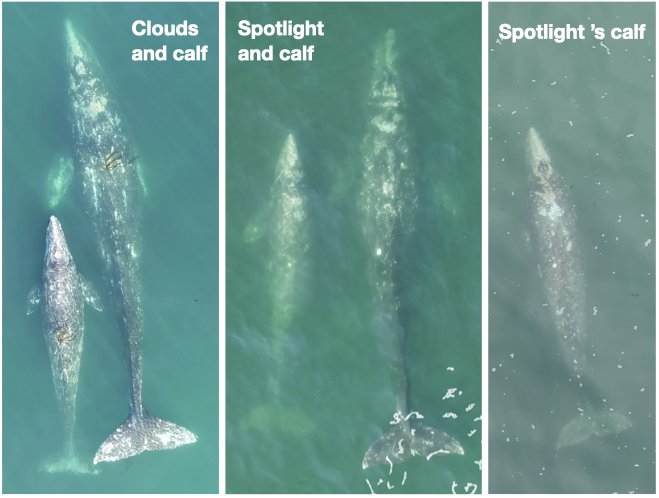
We can monitor space use patterns of individuals in a population through time using spatial capture-recapture techniques. As the name implies, a spatial capture-recapture technique involves capturing an individual in a marked location during a sampling period, releasing it back into the population, and then (hopefully) re-capturing it during another sampling period in the future, at either the same or a different location. With enough repeat sampling events, the method should build spatial capture histories of individuals through time to better understand an individual’s space use patterns (Borchers & Efford 2008). While the use of the word capture implies that the animal is being physically caught, this is not necessarily the case. Individuals can be “captured” in a number of non-invasive ways, including by being photographed, which is how we “capture” individual PCFG gray whales. These capture-recapture methods were first pioneered in terrestrial systems, where camera traps (i.e., cameras that take photos or videos when a motion sensor is triggered) are set up in a systematic grid across a study area (Figure 1; Royle et al. 2009, Gray 2018). Placing the cameras in a grid system ensures that there is an equal distribution of cameras throughout the study area, which means that an animal theoretically has a uniform chance of being captured. However, because we know that individuals within a population make space use decisions differently, we assume that individuals will distribute themselves differently across a landscape, which will manifest as individuals having different centers of their spatial activity. The probability of capturing an individual is highest when a camera trap is at that individual’s activity center, and the cameras furthest away from the individual’s activity center will have the lowest probability of capturing that individual (Efford 2004). By using this principle of probability, the data generated from spatial capture-recapture field methods can be modelled to estimate the activity centers and ranges for all individuals in a population. The overlap of an individual’s activity center and range can then be compared to the spatiotemporal distribution of stressors that an individual may be exposed to, allowing us to determine whether and how an individual has been exposed to each stressor.

While capture-recapture methods were first developed in terrestrial systems, they have been adapted for application to marine populations, which is what I am doing for our GRANITE dataset of PCFG gray whales. Together with a team of committee members and GRANITE collaborators, I am developing a Bayesian spatial capture-recapture model to estimate individual space use patterns. In order to mimic the camera trap grid system, we have divided our central Oregon coast study area into latitudinal bins that are approximately 1 km long. Unfortunately, we do not have motion sensor activated cameras that automatically take photographs of gray whales in each of these latitudinal bins. Instead, we have eight years of boat-based survey effort with whale encounters where we collect photographs of many individual whales. However, as you now know, being able to calculate the probability of detection is important for estimating an individual’s activity center and range. Therefore, we calculated our spatial survey effort per latitudinal bin in each study year to account for our probability of detecting whales (i.e., the area of ocean in km2 that we surveyed). Next, we tallied up the number of times we observed every individual PCFG whale in each of those latitudinal bins per year, thus creating individual spatial capture histories for the population. Finally, using just those two data sets (the individual whale capture histories and our survey effort), we can build models to test a number of different hypotheses about individual gray whale space use patterns. There are many hypotheses that I want to test (and therefore many models that I need to run), with increasing complexity, but I will explain one here.
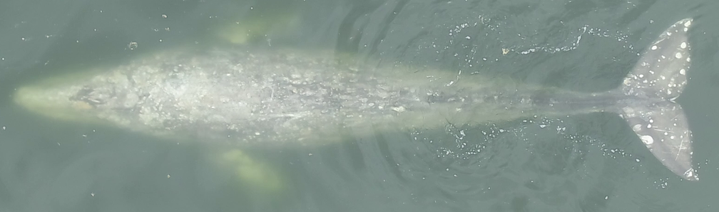
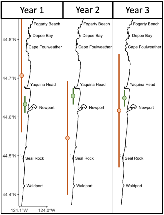
Over eight years of field work for the GRANITE project, consisting of over 40,000 km2 of ocean surveyed with 2,169 sightings of gray whales, our observations lead us to hypothesize that there are two broad space use strategies that whales use to optimize how they find enough prey to meet their energetic needs. For the moment, we are calling these strategies ‘home-body’ and ‘roamer’. As the name implies, a home-body is an individual that stays in a relatively small area and searches for food in this area consistently through time. A roamer, on the other hand, is an individual that travels and searches over a greater spatial area to find good pockets of food and does not generally tend to stay in just one place. In other words, we except a home-body to have a consistent activity center through time and a small activity range, while a roamer will have a much larger activity range and its activity center may vary more throughout the years (Figure 2).
While this hypothesis sounds straightforward, there are a lot of decisions that I need to make in the Bayesian modeling process that can ultimately impact the results. For example, do all home-bodies in a population have the same size activity range or can the size vary between different home-bodies? If it can vary, by how much can it vary? These same questions apply for the roamers too. I have a long list of questions just like these, which means a lot of decision-making on my part, and that long list of hypotheses I previously mentioned. Luckily, I have a fantastic team made up of Leigh, committee members, and GRANITE collaborators that are guiding me through this process. In just a few more months, I hope to reveal how PCFG individuals distribute themselves in space and time throughout our central Oregon study area, and hence describe their exposure to different stressors. Stay tuned!
Did you enjoy this blog? Want to learn more about marine life, research, and conservation? Subscribe to our blog and get a weekly message when we post a new blog. Just add your name and email into the subscribe box below.
References
Borchers DL, Efford MG (2008) Spatially explicit maximum likelihood methods for capture-recapture studies. Biometrics 64:377-385.
Efford M (2004) Density estimation in live-trapping studies. Oikos 106:598-610.
Erlinge S, Sandell M (1986) Seasonal changes in the social organization of male stoats, Mustela erminea: An effect of shifts between two decisive resources. Oikos 47:57-62.
Gray TNE (2018) Monitoring tropical forest ungulates using camera-trap data. Journal of Zoology 305:173-179.
Pirotta E, Booth CG, Costa DP, Fleishman E, Kraus SD, and others (2018) Understanding the population consequences of disturbance. Ecology and Evolution 8(19):9934–9946.Royle J, Nichols J, Karanth KU, Gopalaswamy AM (2009) A hierarchical model for estimating density in camera-trap studies. Journal of Applied Ecology 46:118-127.