By Dawn Barlow, PhD student, OSU Department of Fisheries and Wildlife, Geospatial Ecology of Marine Megafauna Lab
The focus of my PhD research is on the ecology and distribution of blue whales in New Zealand. However, it has been a long time since I’ve seen a blue whale, and much of my time recently has been spent thinking about wind. What does wind matter to a blue whale? It actually matters a whole lot, because the wind drives an important biological process in many coastal oceans called upwelling. Wind blowing along shore, paired with the rotation of the earth, leads to a net movement of surface waters offshore (Fig. 1). As the surface water is pushed away, it is replaced by cold, nutrient-rich water from much deeper. When those nutrients become exposed to sunlight, they provide sustenance for the little planktonic lifeforms in the ocean, which in turn provide food for much larger predators including marine mammals such as blue whales. This “wind-to-whales” trophic pathway was coined by Croll et al. (2005), who demonstrated that off the West Coast of the United States, aggregations of whales could be expected downstream of upwelling centers, in concert with high productivity and abundant krill prey.

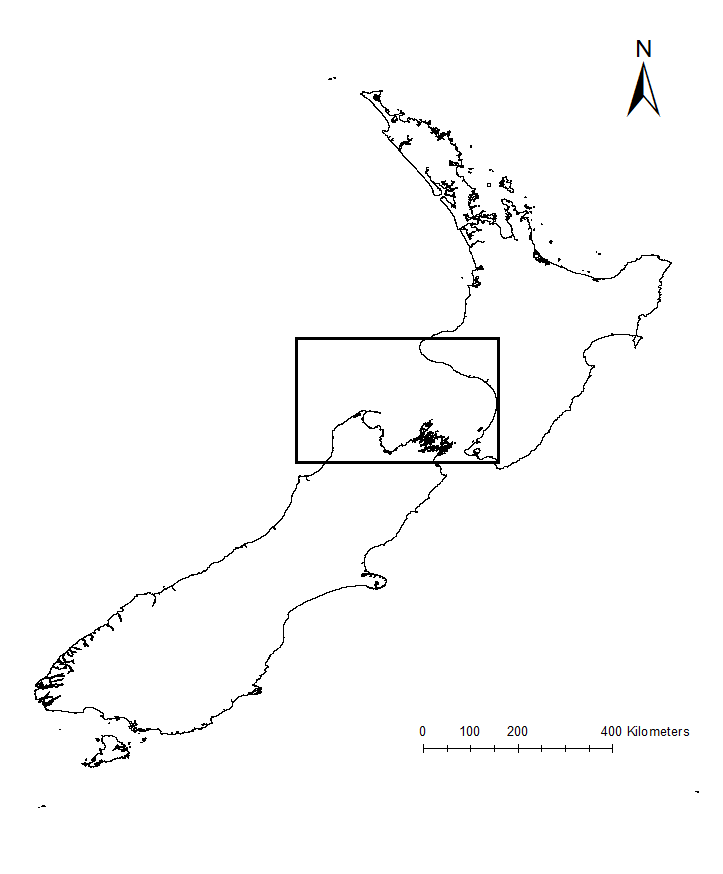
Much of what is understood today about upwelling comes from decades of research on the California Current ecosystem off the West Coast of the United States. Yet, the focus of my research is on an upwelling system on the other side of the world, in the South Taranaki Bight region (STB) of New Zealand (Fig. 2). In the case of the STB, westerly winds over Kahurangi Shoals lead to decreased sea level nearshore, forcing cold, nutrient rich waters to rise to the surface. The wind, along with the persistence of the Westland Current, then pushes a cold and productive plume of upwelled waters around Cape Farewell and into the STB (Fig. 3; Shirtcliffe et al. 1990).

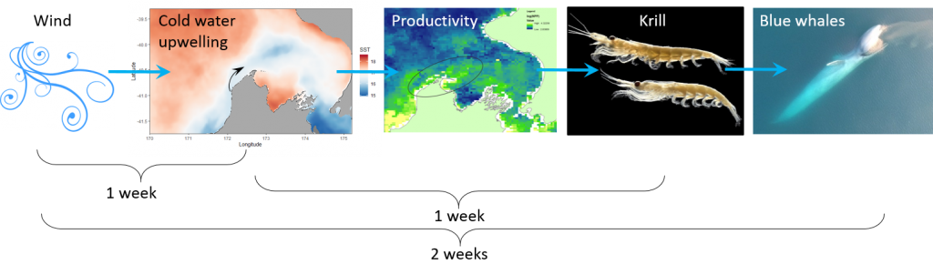
Through research conducted by the GEMM Lab over the years, we have demonstrated that blue whales utilize the STB region for foraging (Torres 2013, Barlow et al. 2018). Recent research on the oceanography of the STB region has further illuminated the mechanisms of this upwelling system, including the path and persistence of the upwelling plume in the STB across years and seasons (Chiswell et al. 2017, Stevens et al. 2019). However, the wind-to-whales pathway has not yet been described for this part of the world, and that is where the next section of my PhD research comes in. The whole system does not respond instantaneously to wind; the pathway from wind to whales takes time. But how much time is required for each step? How long after a strong wind event can we expect aggregations of feeding blue whales? These are some of the questions I am trying to tackle. For example, we hypothesize that some of the mechanisms and their respective lag times can be sketched out as follows:
All of these questions involve integrating oceanography, satellite imagery, wind data, and lag times, leading me to delve into many different analytical approaches including time series analysis and predictive modeling. If we are able to understand the lag times along this series of events leading to blue whale feeding opportunities, then we may be able to forecast blue whale occurrence in the STB based on the current wind and upwelling conditions. Forecasting with some amount of lead time could be a very powerful management tool, allowing for protection measures that are dynamic in space and time and therefore more effective in conserving this blue whale population and balancing human impacts.

References:
Barlow DR, Torres LG, Hodge KB, Steel D, Baker CS, Chandler TE, Bott N, Constantine R, Double MC, Gill P, Glasgow D, Hamner RM, Lilley C, Ogle M, Olson PA, Peters C, Stockin KA, Tessaglia-hymes CT, Klinck H (2018) Documentation of a New Zealand blue whale population based on multiple lines of evidence. Endanger Species Res 36:27–40.
Chiswell SM, Zeldis JR, Hadfield MG, Pinkerton MH (2017) Wind-driven upwelling and surface chlorophyll blooms in Greater Cook Strait. New Zeal J Mar Freshw Res.
Croll DA, Marinovic B, Benson S, Chavez FP, Black N, Ternullo R, Tershy BR (2005) From wind to whales: Trophic links in a coastal upwelling system. Mar Ecol Prog Ser 289:117–130.
Shirtcliffe TGL, Moore MI, Cole AG, Viner AB, Baldwin R, Chapman B (1990) Dynamics of the Cape Farewell upwelling plume, New Zealand. New Zeal J Mar Freshw Res 24:555–568.
Stevens CL, O’Callaghan JM, Chiswell SM, Hadfield MG (2019) Physical oceanography of New Zealand/Aotearoa shelf seas–a review. New Zeal J Mar Freshw Res.
Torres LG (2013) Evidence for an unrecognised blue whale foraging ground in New Zealand. New Zeal J Mar Freshw Res 47:235–248.