By Dawn Barlow, PhD Candidate, OSU Department of Fisheries, Wildlife and Conservation Sciences, Geospatial Ecology of Marine Megafauna Lab
Dynamic forecast models predict environmental conditions and blue whale distribution up to three weeks into the future, with applications for spatial management. Founded on a robust understanding of ecological links and lags, a recent study by Barlow & Torres presents new tools for proactive conservation.
The ocean is dynamic. Resources are patchy, and animals move in response to the shifting and fluid marine environment. Therefore, protected areas bounded by rigid lines may not always be the most effective way to conserve marine biodiversity. If the animals we wish to protect are not within protected area boundaries, then ocean users pay a price without the conservation benefit. Management that is adaptive to current conditions may more effectively match the dynamic nature of the species and places of concern, but this approach is only feasible if we have the relevant ecological knowledge to implement it.
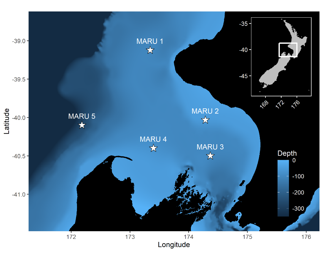
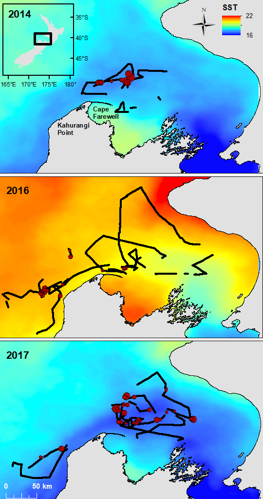
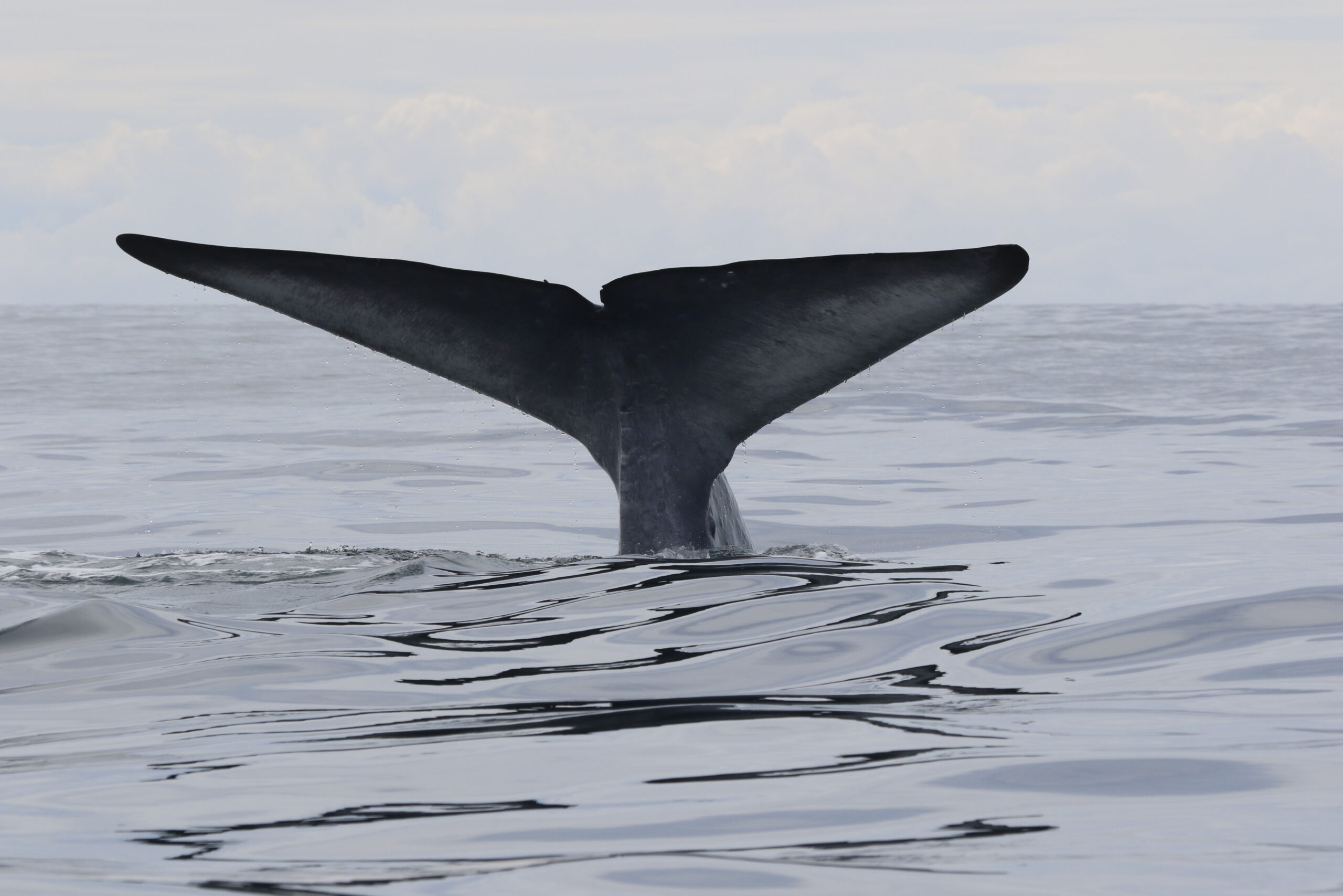
The South Taranaki Bight region of New Zealand is home to a foraging ground for a unique population of blue whales that are genetically distinct and present year-round. The area also sustains New Zealand’s most industrial marine region, including active petroleum exploration and extraction, and vessel traffic between ports.
To minimize overlap between blue whale habitat and human use of the area, we develop and test forecasts of oceanographic conditions and blue whale habitat. These tools enable managers to make decisions with up to three weeks lead time in order to minimize potential overlap between blue whales and other ocean users.

Predicting the future
Knowing where animals were yesterday may not create effective management boundaries for tomorrow. Like the weather, our expectation of when and where to find species may be based on long-term averages of previous patterns, real-time descriptions based on recent data, and forecasts that predict the future using current conditions. Forecasts allow us to plan ahead and make informed decisions needed to produce effective management strategies for dynamic systems.
Just as weather forecasts help us make decisions about whether to wear a raincoat or pack sunscreen before leaving the house, ecological forecasts can enable managers to anticipate environmental conditions and species distribution patterns in advance of industrial activity that may pose risk in certain scenarios.
In our recent study, we develop and test models that do just that: forecast where blue whales are most likely to be, allowing informed decision making with up to three weeks lead time.
Harnessing accessible data for an applicable tool
We use readily accessible data gathered by satellites and shore-based weather stations and made publicly available online. While our understanding of the ecosystem dynamics in the South Taranaki Bight is founded on years of collecting data at-sea and ecological analyses, using remotely gathered data for our forecasting tool is critical for making this approach operational, sustainable, and useful both now and into the future.
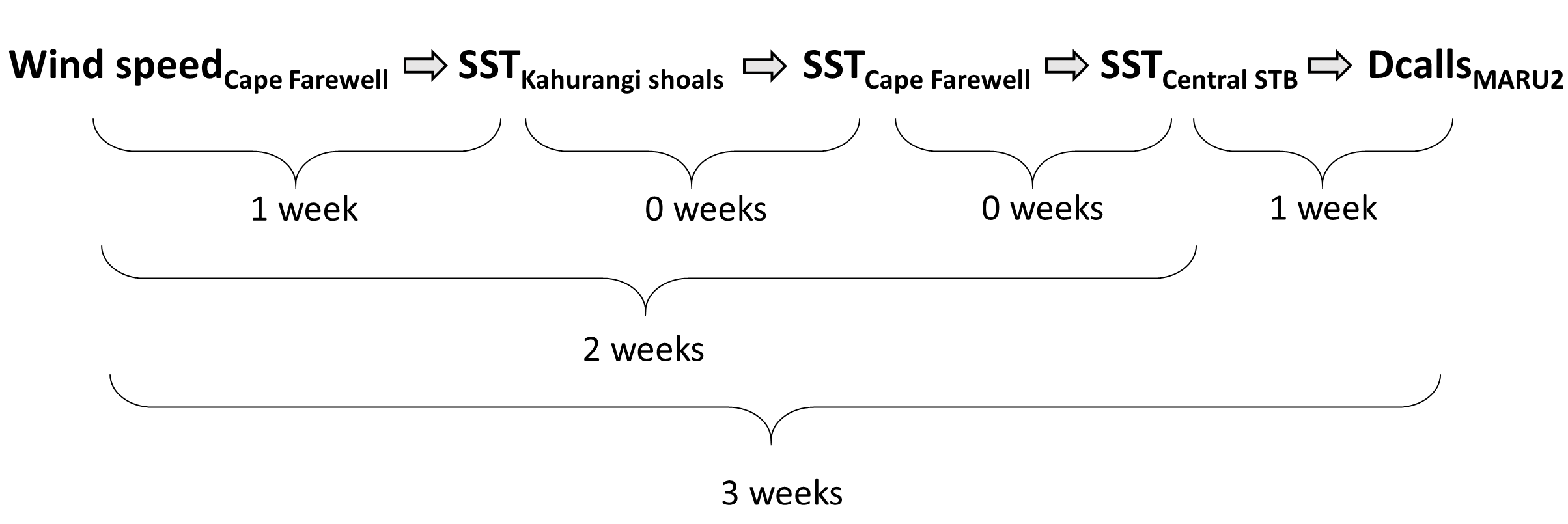
Measurements of conditions such as wind speed and ocean temperature anomaly are paired with known measurements of the lag times between wind input, upwelling, productivity, and blue whale foraging opportunities to produce forecasted environmental conditions.
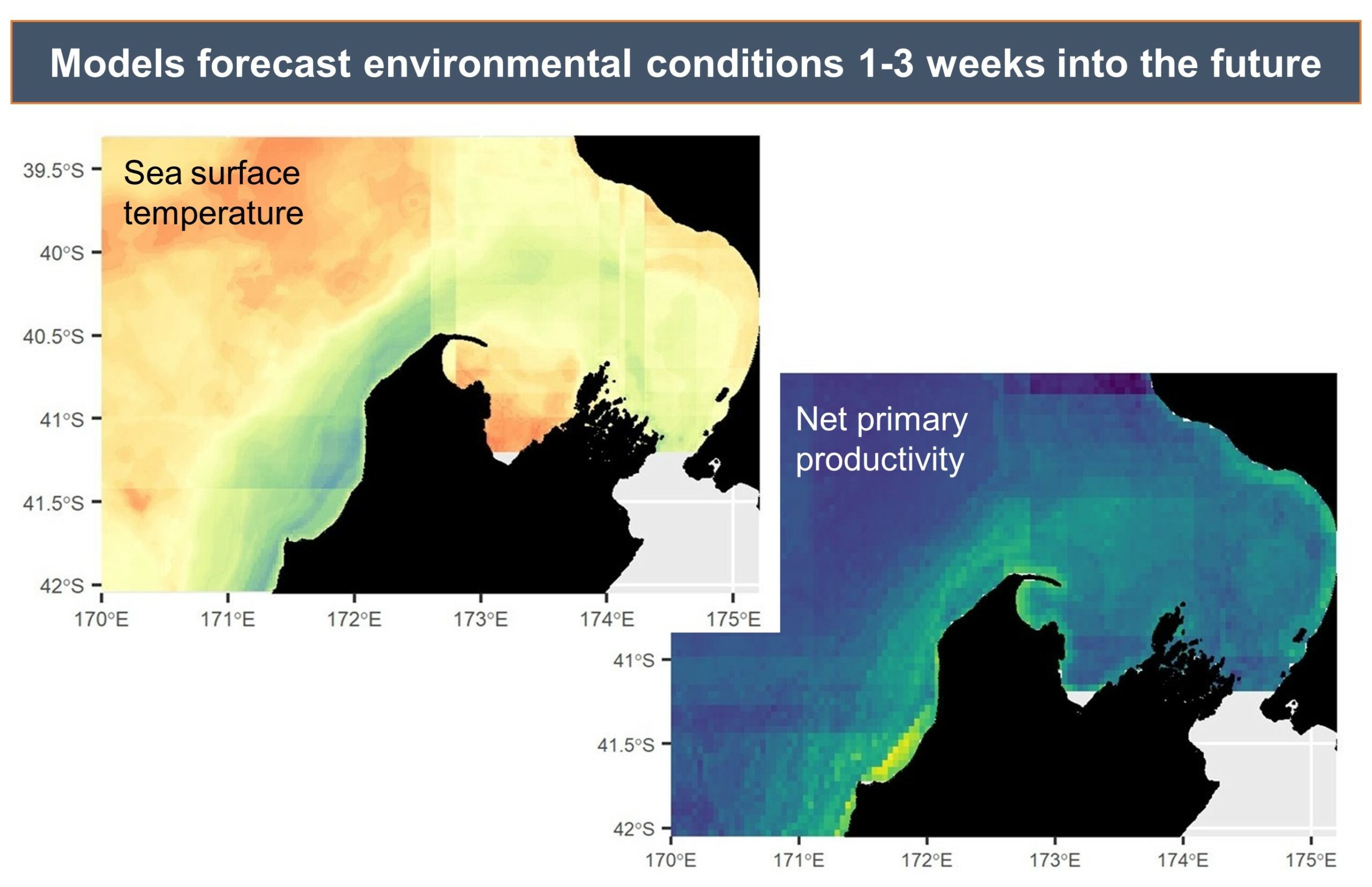
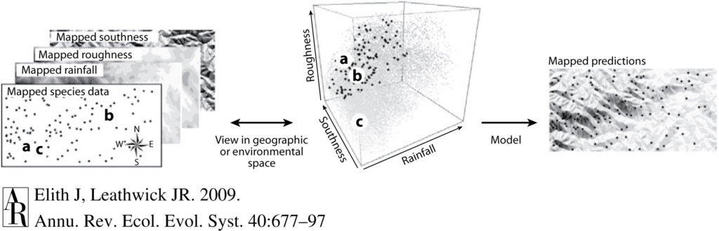
The forecasted environmental layers are then implemented in species distribution models to predict suitable blue whale habitat in the region, generating a blue whale forecast map. This map can be used to evaluate overlap between blue whale habitat and human uses, guiding management decisions regarding potential threats to the whales.

Dynamic ecosystems, dynamic management
These forecasts of whale distribution can be effectively applied for dynamic spatial management because our models are founded on carefully measured links and lags between physical forcing (e.g., wind drives cold water upwelling) and biological responses (e.g., krill aggregations create feeding opportunities for blue whales). The models produce outputs that are dynamic and update as conditions change, matching the dynamic nature of the ecosystem.
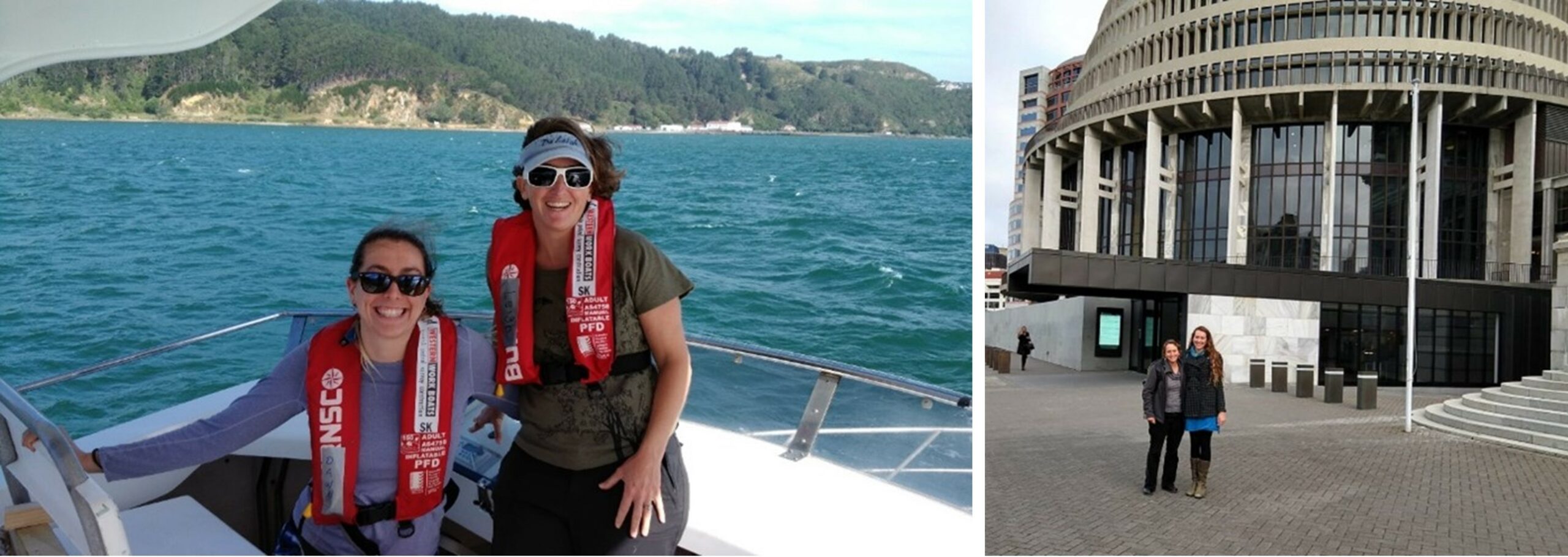
Engagement with stakeholders—including managers, scientists, industry representatives, and environmental organizations—has been critical through the creation and implementation of this forecasting tool, which is currently in development as a user-friendly desktop application.
Our forecast tool provides managers with lead time for decision making and allows flexibility based on management objectives. Through trial, error, success, and feedback, these tools will continue to improve as new knowledge and feedback are received.
Reference: Barlow, D. R., & Torres, L. G. (2021). Planning ahead: Dynamic models forecast blue whale distribution with applications for spatial management. Journal of Applied Ecology, 00, 1–12. https://doi.org/10.1111/1365-2664.13992
This post was written for The Applied Ecologist Blog and the Geospatial Ecology of Marine Megafauna Lab Blog