By Dawn Barlow, PhD student, OSU Department of Fisheries and Wildlife, Geospatial Ecology of Marine Megafauna Lab
In January of 2016, five underwater recording units were dropped to the seafloor in New Zealand to listen for blue whales (Fig. 1). These hydrophones sat listening for two years, brought to the surface only briefly every six months to swap out batteries and offload the data. Through all seasons and conditions when scientists couldn’t be on the water, they recorded the soundscape, generating a wealth of acoustic data with the potential to greatly expand our knowledge of blue whale ecology.

We have established that blue whales are present in New Zealand waters year-round 1. However, many questions remain regarding their distribution across daily, seasonal, and yearly scales. Our two-year acoustic dataset from five hydrophones throughout the STB region is a goldmine of information on blue whale occurrence patterns and the soundscape they inhabit. Having year-round occurrence data will allow us to examine what environmental and anthropogenic factors may influence blue whale distribution patterns. The hydrophones were listening for whales around the clock, every day, while we were on the other side of the world awaiting the recovery of the data to answer our questions.
Before any questions of seasonal distribution or anthropogenic impacts and noise can be addressed, however, we need to know something far more basic: when and where did we record blue whale vocalizations? This may seem like a simple, stepping-stone question, but it is actually quite involved, and the reason I spent the last month working with a team of acousticians at Cornell University’s Center for Conservation Bioacoustics. The expert research group here at Cornell, led by Dr. Holger Klinck, have been instrumental in our New Zealand blue whale research, including developing and building the recording units, hydrophone deployment and recovery, data processing, analysis, and advice. I am thrilled to work with all of them, and had an incredibly productive month of learning about acoustics from the best.
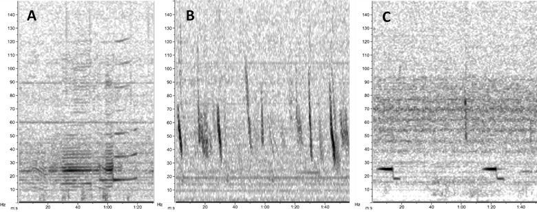
Blue whales produce multiple vocalizations that we are interested in documenting. The New Zealand song (Fig. 2A) is highly stereotyped and unique to the Southwest Pacific Ocean 2,3. Low-frequency downsweeps, or “D calls” (Fig. 2B), are far more variable and produced by blue whale populations around the world 4. Furthermore, Antarctic blue whales produce a highly-stereotyped “Z call” (Fig. 2C) and are known to be present in New Zealand waters occasionally 5.
One way to determine when blue whales were vocalizing is for an analyst to manually review the entirety of the two years of sound recordings for each of the five hydrophones by hand to scan for and select individual vocalizations. An alternative approach is to develop a detector algorithm to locate calls in the data based on their stereotypical characteristics. Over the past month I built, tested, and ran detectors for each blue whale call type using what is called a data template detector. This technique uses example signals from the data that the analyst selects as templates. The templates should be clear signals, and representative of the variation in calls contained in the dataset. Then, by comparing pixel characteristics between the template spectrograms and the spectrogram of the recording of interest using certain matching criteria (e.g. threshold for spectrogram correlation, detection frequency range), the algorithm searches for other signals like the templates in the full dataset. For example, in Fig. 3 you can see units of blue whale song I selected as templates for my detector.

Testing the performance of a detector algorithm is critical. Therefore, a dataset is needed where calls were identified by an analyst and then used as the “ground truth”, to which the detector results are compared. For my ground truth dataset, I took a subset of 52 days and hand-browsed the spectrograms to identify and log New Zealand blue whale song, D calls, and Antarctic Z calls. In evaluating detector performance, there are three important metrics that need to be weighed: precision (the proportion of detections that are true), recall (the proportion of true calls identified by the detector), and false alarm rate (the number of false positive detections per hour). Ideally, the detector should be optimized to maximize precision and recall and minimize the false positives.
The STB region is highly industrial, and our two-year acoustic dataset contains periods of pervasive seismic airgun noise from oil and gas exploration. Ideally, a detector would be able to identify blue whale vocalizations even in the presence of airgun operations that dominate the soundscape for months. For blue whale song, the detector did quite well! With a precision of 0.91 and recall of 0.93, the detector could pick out song units over airgun noise (Fig. 4). A false alarm rate of 8 false positives per hour is a sacrifice worth making to identify song during seismic operations (and the false positives will be removed in a subsequent step). For D calls, seismic survey activity presented a different challenge. While the detector did well at identifying D calls during airgun operation, the first several detector attempts also logged every single airgun blast as a blue whale vocalization—clearly problematic. Through an iterative process of selecting template signals, and adjusting the number of templates used and the correlation threshold, I was able to come up with a detector which selected D calls and missed most airgun blasts. This success felt like a victory.

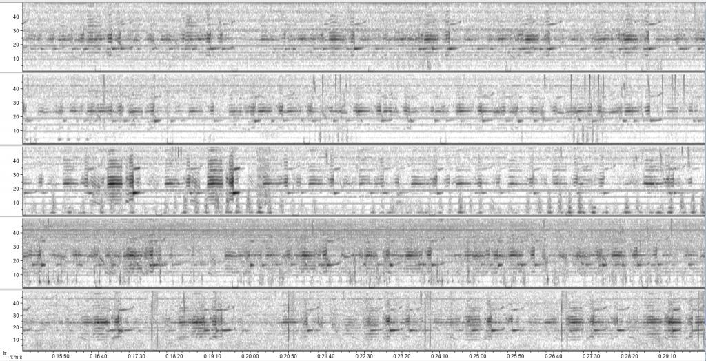
After this detector development and validation process, I ran each detector on the full two-year acoustic dataset for all five recording units. This step was a good exercise in patience as I eagerly awaited the outputs for the many hours they took to run. The next step in the process will be for me to go through and validate each detector event to eliminate any false positives. However, running the detectors on the full dataset has allowed for exciting preliminary examinations of seasonal blue whale acoustic patterns, which need to be refined and expanded upon as the analysis continues. For example, sometimes the New Zealand song dominates the recordings on all hydrophones (Fig. 5), whereas other times of year song is less common. Similarly, there appear to be seasonal patterns in D calls and Antarctic Z calls, with peaks and dips in detections during different times of year.
As with many things, the more questions you ask, the more questions you come up with. From preliminary explorations of the acoustic data my head is buzzing with ideas for further analysis and with new questions I hadn’t thought to ask of the data before. My curiosity has been fueled by scrolling through spectrograms, looking, and listening, and I am as excited as ever to continue researching blue whale ecology. I would like to thank the team at the Center for Conservation Bioacoustics for their support and guidance over the past month, and I look forward to digging deeper into the stories being told in the acoustic data!

References
1. Barlow, D. R. et al. Documentation of a New Zealand blue whale population based on multiple lines of evidence. Endanger. Species Res. 36, 27–40 (2018).
2. McDonald, M. A., Mesnick, S. L. & Hildebrand, J. A. Biogeographic characterisation of blue whale song worldwide: using song to identify populations. J. Cetacean Res. Manag. 8, 55–65 (2006).
3. Balcazar, N. E. et al. Calls reveal population structure of blue whales across the Southeast Indian Ocean and the Southwest Pacific Ocean. J. Mammal. 96, 1184–1193 (2015).
4. Oleson, E. M. et al. Behavioral context of call production by eastern North Pacific blue whales. Mar. Ecol. Prog. Ser. 330, 269–284 (2007).
5. McDonald, M. A. An acoustic survey of baleen whales off Great Barrier Island, New Zealand. New Zeal. J. Mar. Freshw. Res. 40, 519–529 (2006).