
Clara Bird, PhD Student, OSU Department of Fisheries, Wildlife, and Conservation Sciences, Geospatial Ecology of Marine Megafauna Lab
Over six field seasons the GEMM lab team has conducted nearly 500 drone flights over gray whales, equaling over 100 hours of footage. These hours of footage are the central dataset for my PhD dissertation, so it’s up to me to process them all. This process can be challenging, tedious, and daunting, but it is also quite fun and a privilege to be the one person who gets to watch all the footage. It’s fascinating to get to know the whales and their behaviors and pick up on patterns. It motivates me to get through this video processing step and start doing the data analysis. Recently, it’s been especially fun to notice patterns that I’ve seen mentioned in the literature. One example is adult social behavior.
There are two categories of social behavior that I’m interested in studying: maternal behavior, defined as interactions between a mom and its calf, and general social behaviors, defined as social interactions between non-mom/calf pairs. In this blog I’ll focus on general social behaviors, but if you’re interested in maternal behavior check out this blog. General social behavior, which I’ll refer to as social behavior moving forward, includes tactile interactions and promiscuous behaviors (Torres et al. 2018; Clip 1). While gray whales in the PCFG range are primarily foraging, researchers have observed increases in social behavior towards the end of the foraging season (Stelle et al., 2008; Torres et al., 2018). We think that this indicates that the whales are starting to focus less on feeding and more on breeding. This tradeoff of foraging vs. socializing time is interesting because it comes at an energetic cost.
Broadly, animals need to balance the energetic demands of survival with those of reproduction. They need to reproduce to pass on their genes, but reproduction is energetically demanding, and animals also need to survive and grow to be able to reproduce. The decision to reproduce is costly because reproduction requires energetic investment and time investment since animals do not forage (gaining energy) when they are socializing. Consequently, only animals with sufficient energy reserves (i.e., body condition) to invest in reproduction actually engage in reproduction. Given these costs associated with reproduction, we expect to see a relationship between social behavior and body condition (Green, 2001) with mainly animals in good body condition engaging in social behavior because these animals have sufficient reserves to sustain the cost. Furthermore, since body condition is an indicator of foraging success and prey availability, environmental conditions can also affect social behavior and reproduction through this pathway.
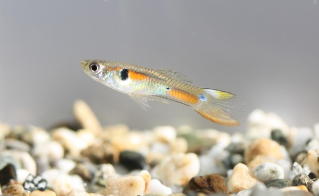
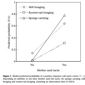
Rahman et al. (2014) used a lab experiment to study the relationship between nutritional stress and male guppy courtship behavior (Figure 1). In their experiment they tested for the effects of both decreased diet quantity and quality on the frequency of male courtship behaviors. Rahman et al (2014) found that individuals in the low-quantity group were significantly smaller than those in the high-quality group and that diet quantity had a significant effect on the frequency of courtship behaviors. Males fed a low-quantity diet performed fewer courtship behaviors. Interestingly, there was no significant effect of diet quality on courtships behavior, although there was some evidence of an interaction effect, which suggests that within the low-quantity group, males fed with high-quality food performed more courtship behaviors that those fed with low-quality food. This study is interesting because it shows how foraging success (diet quantity and quality) can affect courting behavior.
However, guppies are not the ideal species for comparison to gray whales because gray whales and guppies have quite different life history traits. A more fitting comparison would be with an example species with more in common with gray whales, such as viviparous capital breeders. Viviparous animals develop the embryo inside the body and give live birth. Capital breeders forage to build energy reserves and then rely on those energy reserves during reproduction. Surprisingly, I found asp vipers to be a good example species for comparison to gray whales.
Asp vipers (Figure 2) are viviparous snakes who are considered capital breeders because they forage prior to hibernation, and then begin reproduction immediately following hibernation without additional foraging. Naulleau & Bonnet (1996) conducted a field study on female asp vipers to determine if there was a difference in body condition at the start of the breeding season between females who reproduced or not during that season. To do this they marked individuals and measured their body condition at the start of the breeding season and then recaptured those individuals at the end of the breeding season and recorded whether the individual had reproduced. Interestingly, they found that there was a strongly significant difference in body condition between females that did and did not reproduce. In fact, they discovered that no female below a certain body condition value reproduced, meaning that they found a body condition threshold for reproduction.

Additionally, a study on water pythons found that their body condition threshold for reproduction shifted over time in response to prey availability (Madsen & Shine, 1999). These authors found that females lowered their threshold after several consecutive years of poor prey availability. These studies are really exciting to me because they address questions that the GRANITE project team is interested in tackling.
Understanding the relationship between body condition and reproduction in gray whales is an important puzzle piece for our work. The aim of the GRANITE project is to understand how the effects of stressors on individual whales scales up to population level impacts (read Lisa’s blog to learn more). Reproduction rates play a big role in population dynamics, so it is important to understand what factors affect reproduction. Since we’re studying these whales on their foraging grounds, assessing body condition provides an important link between foraging behavior and reproduction.
For example, if an individual’s response to a stressor is to forage less, that may lead to poorer body condition, meaning that they may be less likely to reproduce. While reduced reproduction in one individual may not have a big effect on the population, the same response from multiple individuals could impact the population’s dynamics (i.e., increasing or decreasing abundance). Understanding these different relationships between behavior, body condition, and reproduction rates is a big undertaking, but it’s exciting to be a member of the GRANITE team as this strong group of scientists works to bring together different data streams to work on this big picture question. We’re all deep into data processing right now so stay tuned over the next few years to learn more about gray whale social behavior and to find out if fat whales are more social than skinny whales.
Did you enjoy this blog? Want to learn more about marine life, research, and conservation? Subscribe to our blog and get weekly updates and more! Just add your name into the subscribe box on the left panel.
References
Green, A. J. (2001). Mass/Length Residuals: Measures of Body Condition or Generators of Spurious Results? Ecology, 82(5), 1473–1483. https://doi.org/10.1890/0012-9658(2001)082[1473:MLRMOB]2.0.CO;2
Madsen, T., & Shine, R. (1999). The adjustment of reproductive threshold to prey abundance in a capital breeder. Journal of Animal Ecology, 68(3), 571–580. https://doi.org/10.1046/j.1365-2656.1999.00306.x
Naulleau, G., & Bonnet, X. (1996). Body Condition Threshold for Breeding in a Viviparous Snake. Oecologia, 107(3), 301–306.
Rahman, M. M., Kelley, J. L., & Evans, J. P. (2013). Condition-dependent expression of pre- and postcopulatory sexual traits in guppies. Ecology and Evolution, 3(7), 2197–2213. https://doi.org/10.1002/ece3.632
Rahman, M. M., Turchini, G. M., Gasparini, C., Norambuena, F., & Evans, J. P. (2014). The Expression of Pre- and Postcopulatory Sexually Selected Traits Reflects Levels of Dietary Stress in Guppies. PLOS ONE, 9(8), e105856. https://doi.org/10.1371/journal.pone.0105856
Stelle, L. L., Megill, W. M., & Kinzel, M. R. (2008). Activity budget and diving behavior of gray whales (Eschrichtius robustus) in feeding grounds off coastal British Columbia. Marine Mammal Science, 24(3), 462–478. https://doi.org/10.1111/j.1748-7692.2008.00205.x
Torres, L. G., Nieukirk, S. L., Lemos, L., & Chandler, T. E. (2018). Drone up! Quantifying whale behavior from a new perspective improves observational capacity. Frontiers in Marine Science, 5(SEP). https://doi.org/10.3389/fmars.2018.00319


