Clara Bird, PhD Candidate, OSU Department of Fisheries, Wildlife, and Conservation Sciences, Geospatial Ecology of Marine Megafauna Lab
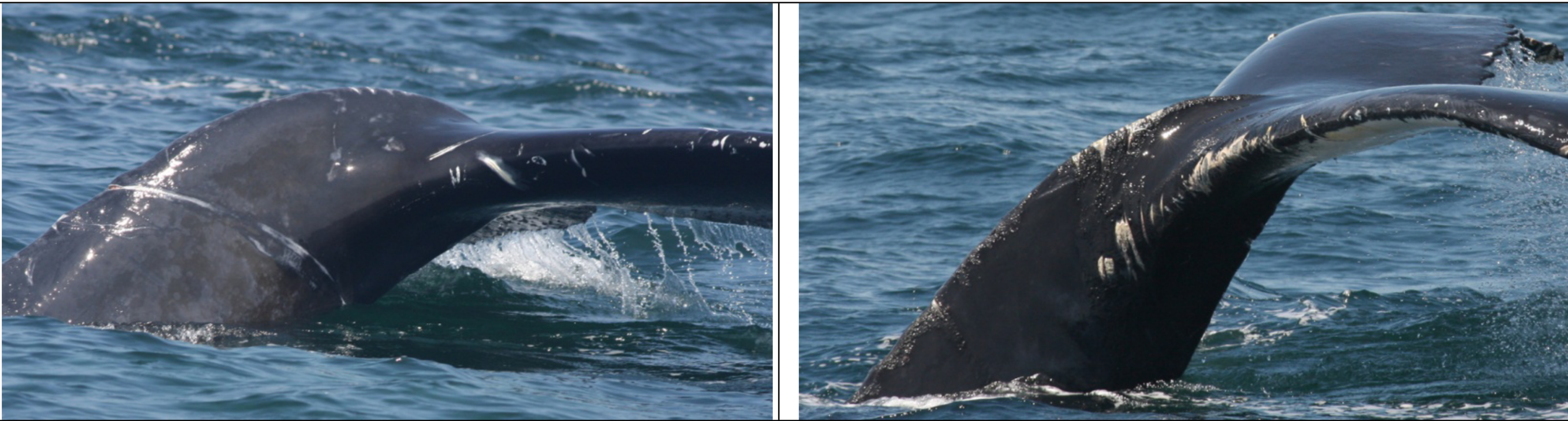
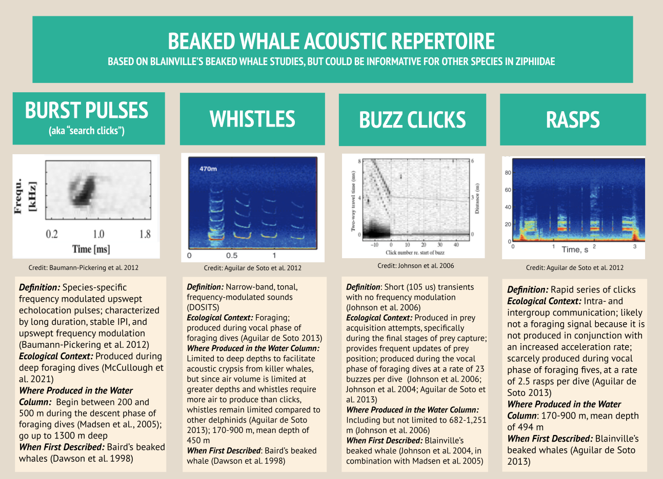
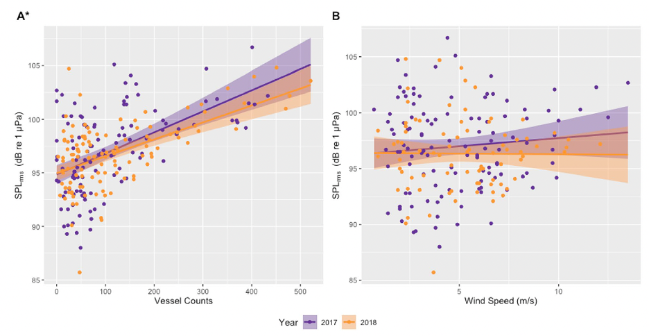
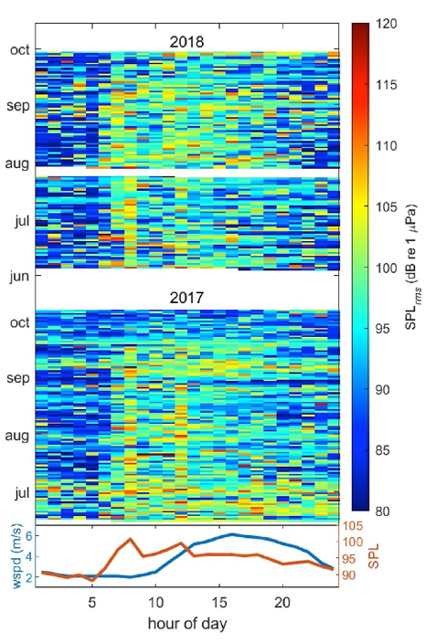
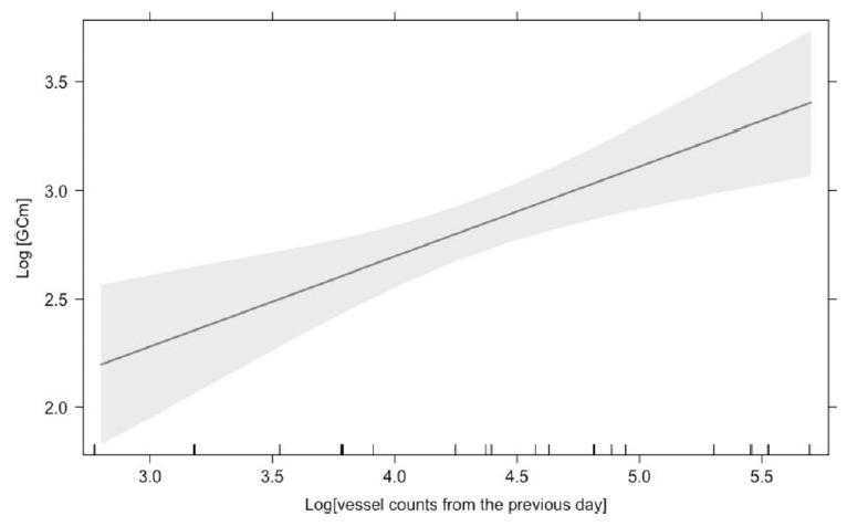
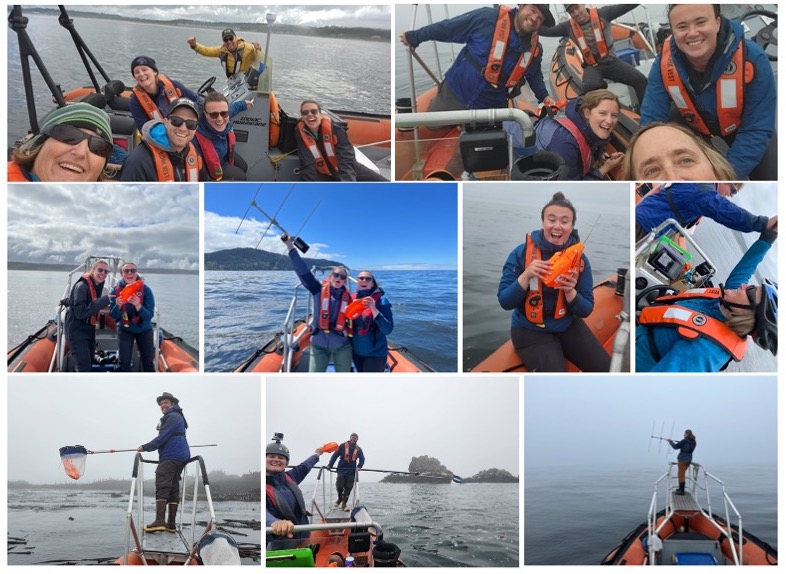
Since its start, the GEMM Lab has been interested in the effect of vessel disturbance on whales. From former student Florence’s masters project to Leila’s PhD work, this research has shown that gray whales on their foraging grounds have a behavioral response to vessel presence (Sullivan & Torres, 2018) and a physiological response to vessel noise (Lemos et al., 2022). Presently, our GRANITE project is continuing to investigate the effect of ambient noise on gray whales, with an emphasis on understanding how these effects might scale up to impact the population as a whole (Image 1).
To date, all this work has been focused on gray whales feeding off the coast of Oregon, but I’m excited to share that this is about to change! In just a few weeks, Leigh and I will be heading south for a pilot study looking at the effects of whale watching vessels on gray whale mom/calf pairs in the nursing lagoons of Baja California, Mexico.

We are collaborating with a Fernanda Urrutia Osorio, a PhD candidate at Scripps Institute of Oceanography, to spend a week conducting fieldwork in one of the nursing lagoons. For this project we will be collecting drone footage of mom/calf pairs in both the presence and absence of whale watching vessels. Our goal is to see if we detect any differences in behavior when there are vessels around versus when there are not. Tourism regulations only allow the whale watching vessels to be on the water during specific hours, so we are hoping to use this regulated pattern of vessel presence and absence as a sort of experiment.

The lagoons are a crucial place for mom/calf pairs, this is where calves nurse and grow before migration, and nursing is energetically costly for moms. So, it is important to study disturbance responses in this habitat since any change in behavior caused by vessels could affect both the calf’s energy intake and the mom’s energy expenditure. While this hasn’t yet been investigated for gray whales in the lagoons, similar studies have been carried out on other species in their nursing grounds.
We can use these past studies as blueprints for both data collection and processing. Disturbance studies such as these look for a wide variety of behavioral responses. These include (1) changes in activity budgets, meaning a change in the proportion of time spent in a behavior state, (2) changes in respiration rate, which would reflect a change in energy expenditure, (3) changes in path, which would indicate avoidance, (4) changes in inter-individual distance, and (5) changes in vocalizations. While it’s not necessarily possible to record all of these responses, a meta-analysis of research on the impact of whale watching vessels found that the most common responses were increases in the proportion of time spent travelling (a change in activity budget) and increased deviation in path, indicating an avoidance response (Senigaglia et al., 2016).
One of the key phrases in all these possible behavioral responses is “change in ___”. Without control data collected in the absence of whale watching vessels, it impossible to detect a difference. Some studies have conducted controlled exposures, using approaches with the research vessel as proxies for the whale watchers (Arranz et al., 2021; Sprogis et al., 2020), while others use the whale watching operators’ daily schedule and plan their data collection schedule around that (Sprogis et al., 2023). Just as ours will, all these studies collected data using drones to record whale behavior and made sure to collect footage before, during, and after exposure to the vessel(s).
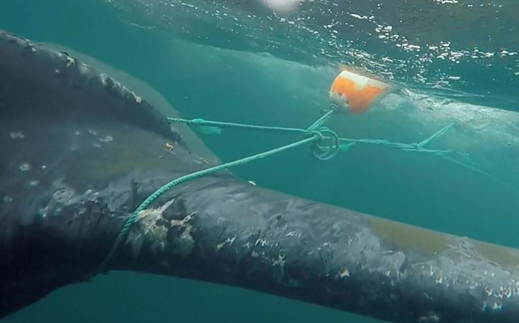
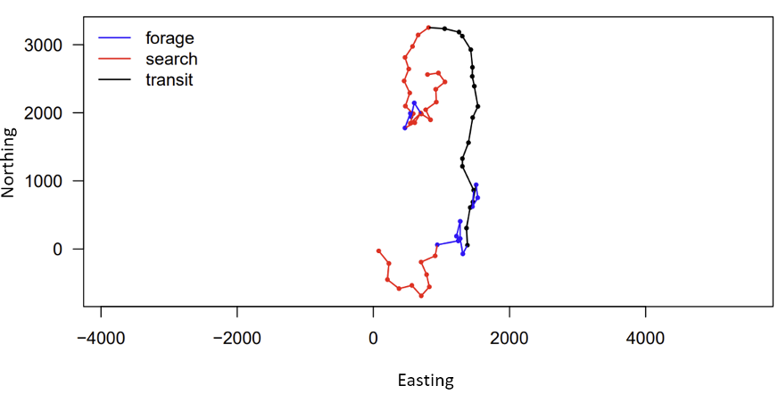
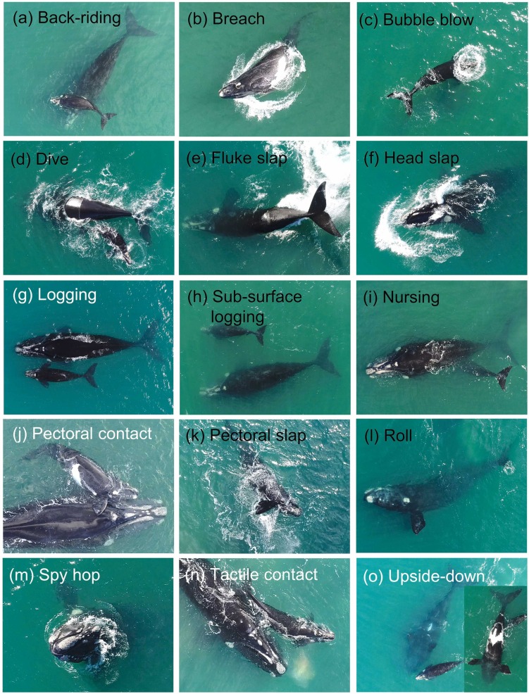
One study focused on humpback mom/calf pairs found a decrease in the proportion of time spent resting and an increase in both respiration rate and swim speed during the exposure (Sprogis et al., 2020). Similarly, a study focused on short-finned pilot whale mom/calf pairs found a decrease in the mom’s resting time and the calf’s nursing time (Arranz et al., 2021). And, Sprogis et al.’s study of Southern right whales found a decrease in resting behavior after the exposure, suggesting that the vessels’ affect lasted past their departure (Sprogis et al., 2023, Image 3). It is interesting that while these studies found changes in different response metrics, a common trend is that all these changes suggest an increase in energy expenditure caused by the disturbance.
However, it is important to note that these studies focused on short term responses. Long term impacts have not been thoroughly estimated yet. These studies provide many valuable insights, not only into the response of whales to whale watching, but also a look at the various methods used. As we prepare for our fieldwork, it’s useful to learn how other researchers have approached similar projects.
I want to note that I don’t write this blog intending to condemn whale watching. I fully appreciate that offering the opportunity to view and interact with these incredible creatures is valuable. After all, it is one of the best parts of my job. But hopefully these disturbance studies can inform better regulations, such as minimum approach distances or maximum engine noise levels.
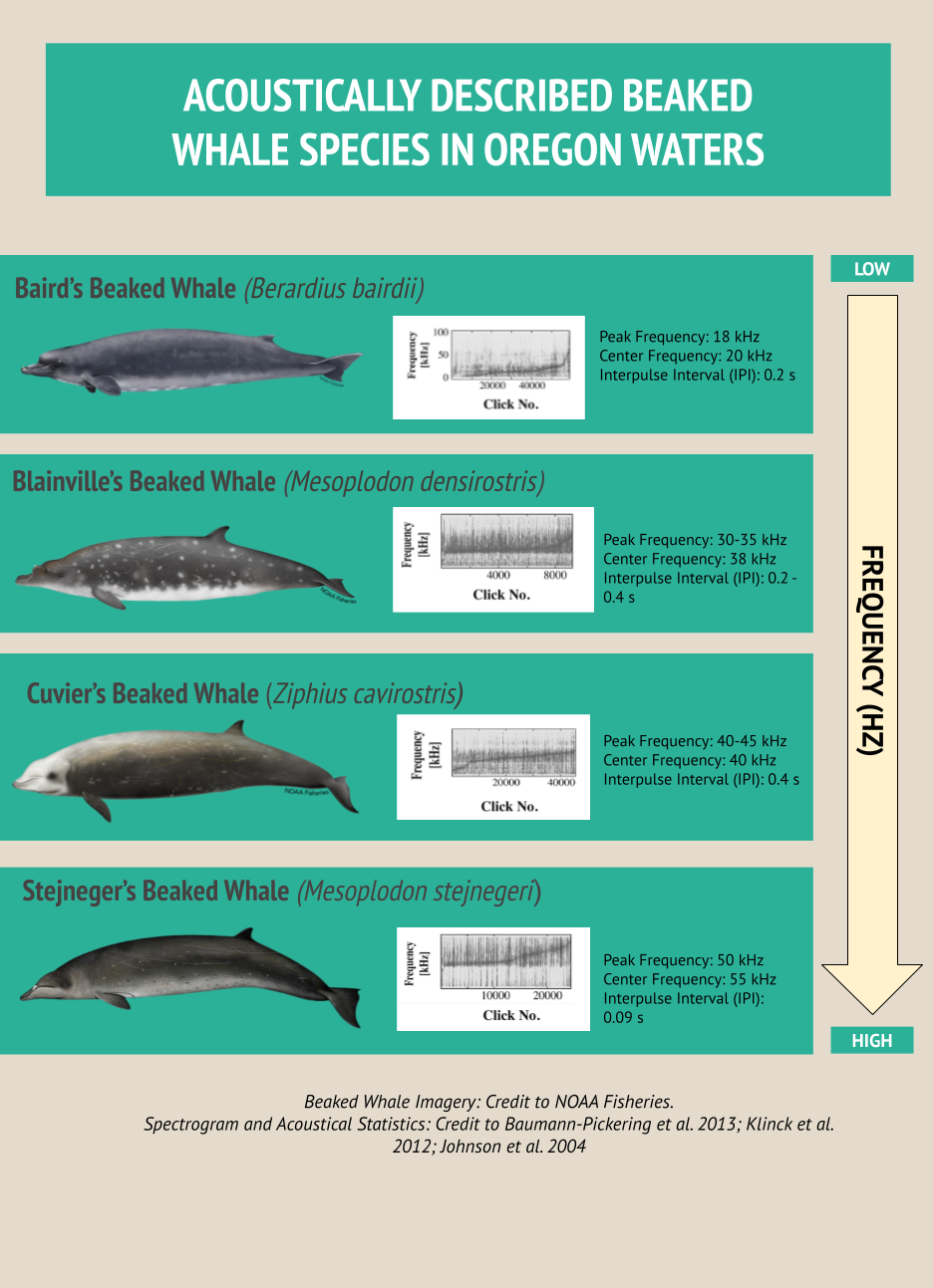
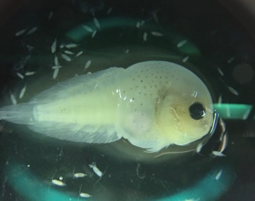
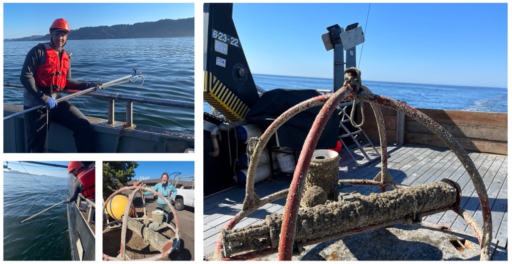
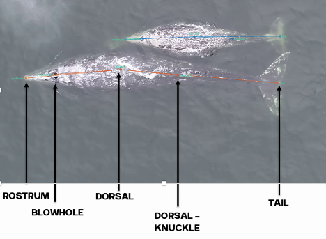
As these studies have done, our first step will be to establish an ethogram of behaviors (our list of defined behaviors that we will identify in the footage) using our pilot data. We can also record respiration and track line data. An additional response that I’m excited to add is the distance between the mom and her calf. Former GEMM Lab NSF REU intern Celest will be rejoining us to process the footage using the AI method she developed last summer (Image 4). As described in her blog, this method tracks a mom and calf pair across the video frames, and allows us to extract the distance between them. We look forward to adding this metric to the list and seeing what we can glean from the results.
While we are just getting started, I am excited to see what we can learn about these whales and how best to study them. Stay tuned for updates from Baja!
Did you enjoy this blog? Want to learn more about marine life, research, and conservation? Subscribe to our blog and get a weekly alert when we make a new post! Just add your name into the subscribe box below!
References
Arranz, P., Glarou, M., & Sprogis, K. R. (2021). Decreased resting and nursing in short-finned pilot whales when exposed to louder petrol engine noise of a hybrid whale-watch vessel. Scientific Reports, 11(1), 21195. https://doi.org/10.1038/s41598-021-00487-0
Lemos, L. S., Haxel, J. H., Olsen, A., Burnett, J. D., Smith, A., Chandler, T. E., Nieukirk, S. L., Larson, S. E., Hunt, K. E., & Torres, L. G. (2022). Effects of vessel traffic and ocean noise on gray whale stress hormones. Scientific Reports, 12(1), Article 1. https://doi.org/10.1038/s41598-022-14510-5
Senigaglia, V., Christiansen, F., Bejder, L., Gendron, D., Lundquist, D., Noren, D., Schaffar, A., Smith, J., Williams, R., Martinez, E., Stockin, K., & Lusseau, D. (2016). Meta-analyses of whale-watching impact studies: Comparisons of cetacean responses to disturbance. Marine Ecology Progress Series, 542, 251–263. https://doi.org/10.3354/meps11497
Sprogis, K. R., Holman, D., Arranz, P., & Christiansen, F. (2023). Effects of whale-watching activities on southern right whales in Encounter Bay, South Australia. Marine Policy, 150, 105525. https://doi.org/10.1016/j.marpol.2023.105525
Sprogis, K. R., Videsen, S., & Madsen, P. T. (2020). Vessel noise levels drive behavioural responses of humpback whales with implications for whale-watching. ELife, 9, e56760. https://doi.org/10.7554/eLife.56760
Sullivan, F. A., & Torres, L. G. (2018). Assessment of vessel disturbance to gray whales to inform sustainable ecotourism. Journal of Wildlife Management, 82(5), 896–905. https://doi.org/10.1002/jwmg.21462