By Elizabeth Kelly, Pacific High School senior, GEMM Lab summer intern
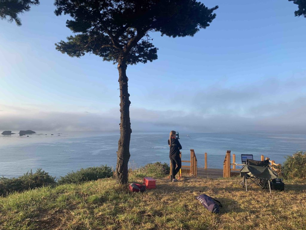
Figure 1. Liz on the cliff. Source: E. Kelly.
The gray whale foraging ecology project with OSU’s GEMM Lab has been nothing short of a dream come true. Going into this internship, I was just a high schooler who had taken zoology my previous school year. With my lack of a formal education in marine biology, let alone gray whales, I was a little daunted at the thought of going to a university field station with college students and actual biologists. When I applied for this internship, I didn’t think I was even going to be accepted for the internship, but I applied with high hopes and a lot of excitement. When I was officially accepted, I wanted to start immediately.
Despite my concerns of the steep learning curves I knew I would have to overcome, I was ready to jump right into the internship. The other interns live at the field station since they do not live locally, but I drive to the field station every morning because I live about 20 minutes away. However, this situation has never made me feel like an outsider. I spend a lot of my time at the field station and it would be hard to not get comfortable there immediately. I don’t feel sad that somebody is cooking some sort of delicious meal every night because even though I don’t live at the station, I sometimes stay for dinners. When I’m there for whatever reason, whether it be while working or eating and hanging out after a day of working or during breaks, I never feel out of my depth socially or even academically even though I am clearly younger and less experienced. The environment and team here, which is made up of scholarly individuals with lots of personality and character, is never judgemental or patronizing; rather it is inviting and the graduate student intern, Noah, and my team leader, Lisa, give off a feeling of mentorship. This has made my internship fun and given me far more of an interest and intent towards pursuing Wildlife Sciences after high school.
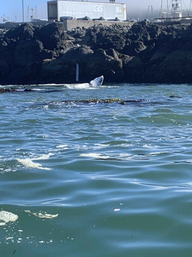
Figure 2. A photo taken by Liz today on the cliff as a whale traveled from Tichenor Cove to Mill Rocks. Source: GEMM Lab.
While there have been tedious parts of the internship with a steep learning curve, including asking many questions about whales, and learning to use different programs, tools and methods, it all pays off and comes in handy when the whole focus of the work comes through town – the famous gray whales. During this field season we have been having low whale sightings for the first 4 weeks (but our sightings are slowly picking up over the last couple days), so the waiting for the grand appearance of a whale can feel eternal. Though, when the red curtains reveal a blow out in the distance headed our way, the feeling of boredom when staring at the ocean is completely forgotten. Suddenly, everyone jumps to action – the theodolite’s position needs to be adjusted as we try to pinpoint where the whale will surface next after its dive.
Figure 3. A zoomed-in photo from the kayak of a gray whale headstanding (a feeding behavior) in Tichenor Cove. Source: E. Kelly.
Recently we have been collecting larger samples of zooplankton when sampling from our research kayak, and the whales have been coming in larger numbers too. Every time I see a whale while I am out on the kayak I am crippled with excitement and adrenaline. There is absolutely nothing like seeing these majestic mammals out and about in their day-to-day lives. I love when I get to see them forage, blow, shark, and even do headstands in the water. When we see them forage in a spot that is not one of our regular zooplankton sampling stations we do some adaptive sampling (sampling at spots where we see whales actively feeding), and so far the whales haven’t lied to me about where the zooplankton is. I’m very curious as to how the whales know where the higher concentrations of zooplankton are, even in low visibility (we have had plenty of that this year too). Nevertheless, they know and aren’t shy about getting what they want.
The only downfall of this internship is that it ends soon. I have thoroughly enjoyed my time with my team and at the field station. This in-the-field experience is one of a kind. Even though I didn’t think I was going to receive this internship, I really wanted it and now that I have had it and am finishing up with it, I am so grateful for the knowledge and experiences I have gained from it and look forward to the opportunities it will further grant me.
By Mattea Holt Colberg, GEMM Lab summer intern, OSU junior
Science is about asking new questions in order to make new discoveries. Starting every investigation with a question, sparked by an observation, is enshrined in the scientific method and pursued by researchers everywhere. Asking questions goes beyond scientific research though; it is the best way to learn new things in any setting.
When I first arrived in Port Orford, I did not know much about gray whales. The extent of my knowledge was that they are large baleen whales that migrate every year and feed on plankton. I did, however, know quite a bit about killer whales. I have been interested in killer whales since I was 5 years old, so I have spent years reading about, watching, and listening to them (my current favorite book about them is Of Orcas and Men, by David Neiwert and I highly recommend it!). I have also had opportunities to research them in the Salish Sea, both on a sailing trip and through the dual-enrollment program Ocean Research College Academy, where I explored how killer whales respond to ambient underwater noise for a small independent project. Knowing more about killer whales than other species has caused killer whales to be the lens through which I approach learning and asking questions about other whales.
Figure 1a. Killer whales traveling in a group in the Salish Sea. Source: ISTOCK.
Figure 1b. A gray whale traveling solo in Tichenor Cove. Source: GEMM Lab.
At first, I was not sure how to apply what I know about killer whales specifically to research on gray whales, since killer whales are toothed whales, while gray whales are baleen whales. There are several differences between toothed whales and baleen whales; toothed whales tend to be more social, occurring in pods or groups, eat larger prey like fish, squid, and seals, and they echolocate. In comparison, baleen whales are less social, eat mostly tiny zooplankton prey, and do not echolocate. Because of these differences, I wanted to learn more about gray whales, so I started asking Lisa questions. Killer whales only sleep with half of their brain at a time, so I asked if gray whales do the same. They do. Killer whales typically travel in stable, long-term matriarchal groups, and I recently learned that gray whales frequently travel alone (though not exclusively). This new knowledge to me led me to ask if gray whales vocalize while traveling. They typically do not. Through asking these questions, and others, I have begun to learn more about gray whales.
Figure 2. Mattea on the tandem research kayak taking a break in between prey sampling. Source: L. Hildebrand.
I am still learning about marine mammal research, and from what I have experienced so far, marine mammal acoustics intrigues me the most. As a child, I developed a general interest in whale vocalizations after hearing recordings of them in museums and aquariums. Then, two years ago, I heard orcas vocalizing in the wild, and I decided I wanted to learn more about their vocalizations as a long-term career goal.
To pursue a career studying marine mammal acoustics, I will need scientific and communication skills that this internship is helping me develop. Sitting on the cliff for hours at a time, sometimes with gray whales swimming in our view-scape and sometimes without, is teaching me the patience and attention needed to review hours of sound recordings with or without vocalizations. Identifying and counting zooplankton most days is teaching me the importance of processing data regularly, so it does not build up or get too confusing, as well as attention to detail and keeping focused. Collecting data from a kayak is teaching me how to assess ocean conditions, keep track of gear, and stay calm when things go wrong. I am also practicing the skill of taking and identifying whale photos, which can be applied to many whale research topics I hope to pursue. Through writing this blog post and discussing the project with Lisa and my fellow interns, I am improving my science communication skills.
Figure 3. Mattea manning the theodolite watching and waiting for a gray whale to show up in our study area. Source: L. Hildebrand.
As an undergraduate student, it can sometimes be difficult to find opportunities to research marine mammals, so I am very grateful for and excited about this internship, both because of the skills it is helping me build and the field work experiences that I enjoy participating in. Another aspect of research this internship is helping me learn about is to ask engaging questions. As I mentioned at the beginning of this post, asking questions is a key element of conducting research. By asking questions about gray whales based on both prior knowledge and new observations, I am practicing this skill, as well as thinking of topics I am curious about and might want to explore in the future. While watching for whales, I have thought of questions such as: How is whale behavior affected by surface conditions? Do gray whales prefer feeding at certain times of the day? Questions like these help me learn about whales, and they keep me excited about research. Thanks to this internship, I can continue working towards my dreams of pursuing similar questions about whales as a career.
Yodel-Ay-Ee-Ooooo! Hello from the Theyodelers, this year’s Port Orford gray whale foraging ecology field team. In case you were wondering, no, we aren’t hobby yodelers and we don’t plan on becoming them. The team name this year actually has to be attributed to a parent of one of my interns. Shout out to Scott Holt who during the first week of the field season asked his daughter Mattea (our OSU undergraduate intern) whether using a theodolite (the instrument we use to track gray whales from our cliff site) is anything like yodeling. The name was an immediate hit with the team and so the team name discussion was closed fairly early on in the season. Now that I have explained our slightly unconventional team name, let me tell you a little about this year’s team and what has been going on down here on the Oregon south coast so far.
As you can tell from the byline, I (Lisa) am back as the project’s team lead in this, the 6th year of the Port Orford gray whale research and internship project. Going into this year’s field season with two years of experience under my belt has made me feel more confident and comfortable with diving straight back into our fine-scale research with a new team of interns. Yet, I am beginning to realize that no matter how much experience I have, there will always be unforeseeable curve balls thrown at me that I can’t anticipate no matter how prepared or experienced I am. However, my knowledge and experience now certainly inform how I tackle these curve balls and hopefully allow my problem-solving to be better and quicker. I am so thrilled that Leigh and I were able to get the field season approved here in Port Orford despite the ongoing pandemic. There were many steps we had to take and protocols to write and get approved, but it was worth the work. It certainly is strange living in a place that is meant to be your home for six weeks but having to wear a face covering everywhere except your own bedroom. However, mask wearing, frequent hand washing, and disinfecting is a very small price to pay to avoid having a lapse in our gray whale data collected here in Port Orford (and minimize transmission). Doing field research amidst COVID has certainly been a big curve ball this year but, so far, I have been able to handle these added challenges pretty well, especially with a lot of help from my team. Speaking of which, time to introduce the other Theyodelers…
Figure 1. Noah watching and waiting for whales on the cliff. When we are outside in the wind and are able to maintain a minimum 6-ft distance, we are able to remove our face coverings. Source: T. McCambridge.
First up, we have Noah Dolinajec. Noah is a fellow graduate student who is currently doing a Master’s in Marine & Lacustrine Science and Management at the Vrije Universiteit Brussel in Brussels, Belgium. While he is attending graduate school in Belgium, Noah is not actually from this European country. In fact, he is a Portlandian! As an Oregonian with a passion for the marine environment, Noah is no stranger to the Oregon coast and has spent quite some time exploring it in the past. Some other things about Noah: before going to college he played semi-professional ice hockey, he is a bit of a birder, and he likes to cook (he and I have been tag-teaming the team cooking this year).
Figure 2. Mattea outside the field station holding local fisher-pup Jim.Source: L. Hildebrand.
Next, we have Mattea Holt Colberg. As I mentioned before, Mattea is the team’s OSU undergraduate intern this year. By participating in a running-start program at her high school where she took two years of college classes, Mattea entered OSU as a junior at just 18 years old! However, she has decided to somewhat extend her undergraduate career at OSU by completing a dual major in Biology and Music. She plays the piano and the violin (which she brought to Port Orford, but we have yet to be serenaded by her). Mattea has previously conducted field research on killer whales in the Salish Sea and I can tell that she is hoping for killer whales to show up in Port Orford (while not entirely ludicrous, the chance of this happening is probably very, very slim).
Figure 3. Liz in the bow of the kayak in Tichenor Cove.Source: L. Hildebrand.
Last but certainly not least, is Liz Kelly, our Pacific High School intern from Port Orford. Liz has lived in several different states across the country (I’m talking Kentucky to Florida) and so I am really excited that she currently lives here in Oregon because she has been an absolute joy to have on the team so far. Liz brings a lot of energy and humor to the team, which we have certainly needed whenever those curve balls come flying. Besides her positivity, Liz brings a lot of determination and perseverance and seeing her work through tough situations here already has made me very proud. I really hope this internship provides Liz with the life, STEM, and communication skills she needs to help her succeed in pursuing her goals of doing wildlife research after college. As you may have read in my last blog, our previous high school interns have had successes in being admitted to various colleges to follow their goals, and I feel confident that Liz will be no different. When she is not here at the field station, she can probably be found taking care of and riding one of her four horses (Millie, Maricja, Miera, and Jeanie).
Now that I have introduced the 2020 field team, here is a short play-by-play of what we have been seeing, or perhaps more aptly, not seeing. Our whale sighting numbers have been pretty low so far and when we do see them, they seem to be foraging a little further away from our study site than I am used to seeing in past years. However, this shift in behavior is not entirely surprising to me since our zooplankton net has been coming up pretty empty at our sampling stations. While there are mysids and amphipods scattered here and there, their numbers are in the low 10s when we do our zooplankton ID lab work in the afternoons. These low counts are also reflected by the low densities I am anecdotally seeing on our GoPro drops (Fig 4).
Figure 4. Comparison of zooplankton density from our GoPro videos. Both images were taken at the same sampling station (Tichenor Cove 8), however the image on the left that contains a lot of little critters is from 2018, whereas the image on the right is from last week. This year our drops have been looking more like the image on the right, though typically with even fewer zooplankton.
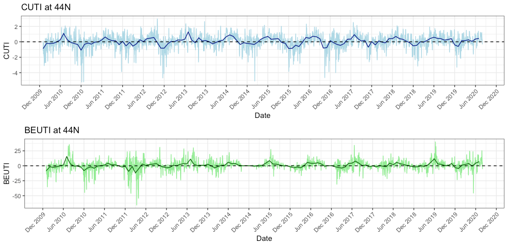
While I am not entirely certain why we are seeing this low prey abundance, I do have some hypotheses. The most likely reason is that this year we experienced some delayed upwelling on our coast. Dawn wrote a great blog about upwelling and wind a few weeks ago and I suggest checking it out to better understand what upwelling is and how it can affect whales (and the whole ecosystem). Typically, we see our peak upwelling occur here in Oregon in May-June. However, if you look at Figure 5 you will see that both the indices remained low at that time this year, whereas in previous years, they were already increasing by May/June.
Figure 5. 10 year time series of the Coastal Upwelling Transport Index (CUTI; top plot) and Biologically Effective Upwelling Transport Index (BEUTI; bottom plot) at 44ºN. CUTI represents the amount of upwelling (positive numbers) or downwelling (negative numbers) while BEUTI estimates the amount of nitrate (i.e. nutrients) upwelled (positive numbers) and downwelled (negative numbers). The light-colored lines representthe CUTI and BEUTI at that point in time while the dark, bold lines represent the long-term average.
A delayed upwelling means that there was likely less nutrients in the water to support little critters like zooplankton to start reproducing and increasing their abundances. Simply put, it means our coastal waters appear to be less productive than they usually are at this time of the year. If there is not much prey around (as we have been finding in our two study sites – Mill Rocks and Tichenor Cove), then it makes sense to me why gray whales are not hanging around since there is not much to feed on. Fortunately, the tail of the trend line in Figure 5 is angling upward, which means that the upwelling finally started in June so hopefully the nutrients, zooplankton and whales will follow soon too. In fact, since I wrote the draft of this blog at the end of last week, we have actually seen an increase in the numbers of mysids in our zooplankton net and on our GoPro videos.
We are almost halfway done with the field season already and I cannot believe how quickly it goes by! During the first two weeks we were busy getting familiar with all of our gear and completing First Aid/CPR and kayak paddle & rescue courses. This week the team started the real data collection. We have had some hiccups (we lost our GoPro stick and our backup GoPro stick, but thankfully have already recovered one of them) but overall, we are off to a pretty good start. Now we just need the upwelling to really kick in, for there to be thick layers of mysids, and for the whales to come in close. Over the next three weeks, you will be hearing from Noah, Mattea and Liz as they share their experiences and viewpoints with all of you!
Clara Bird, Masters Student, OSU Department of Fisheries and Wildlife, Geospatial Ecology of Marine Megafauna Lab
The field season can be quite a hectic time of year. Between long days out on the water, trouble-shooting technology issues, organizing/processing the data as it comes in, and keeping up with our other projects/responsibilities, it can be quite overwhelming and exhausting.
But despite all of that, it’s an incredible and exciting time of year. Outside of the field season, we spend most of our time staring at our computers analyzing the data that we spend a relatively short amount of time collecting. When going through that process it can be easy to lose sight of why we do what we do, and to feel disconnected from the species we are studying. Oftentimes the analysis problems we encounter involve more hours of digging through coding discussion boards than learning about the animals themselves. So, as busy as it is, I find that the field season can be pretty inspiring. I have recently been looking through our most recent drone footage of gray whales and feeling renewed excitement for my thesis.
At the moment, my thesis has four central questions: (1) Are there associations between habitat type and gray whale foraging tactic? (2) Is there evidence of individualization? (3) What is the relationship between behavior and body condition? (4) Do we see evidence of learning in the behavior of mom and calf pairs? As I’ve been organizing my thoughts, what’s become quite clear is how interconnected these questions are. So, I thought I’d take this blog to describe the potential relationships.
Let’s start with the first question: are there associations between habitat types and gray whale foraging tactics? This question is central because it relates foraging behavior to habitat, which is ultimately associated with prey. This relationship is the foundation of all other questions involving foraging tactics because food is necessary for the whales to have the energy and nutrients they need to survive. It’s reasonable to think that the whales are flexible and use different foraging tactics to eat different prey that live in different habitats. But, if different prey types have different nutritional value (this is something that Lisa is studying right now; check out the COZI project to learn more), then not all whales may be getting the same nutrients.
The next question relates to the first question but is not necessarily dependent on it. It’s the question of individualization, a topic Lisa also explored in a past blog. Within our Oregon field sites we have documented a variety of gray whale foraging tactics (Torres et al. 2018; Video 1) but we do not know if all gray whales use all the tactics or if different individuals only use certain tactics. While I think it’s unlikely that one whale only uses one tactic all the time, I think we could see an individual use one tactic more often than the others. I reason that there could be two reasons for this pattern. First, it could be a response to resource availability; certain tactics are more efficient than others, this could be because the tactic involves capturing the more nutritious prey or because the behavior is less energetically demanding. Second, foraging tactics are socially learned as calves from their mothers, and hence individuals use those learned tactics more frequently. This pattern of maternally inherited foraging tactics has been documented in other marine mammals (Mann and Sargeant 2009; Estes et al. 2003). These questions between foraging tactic, habitat and individualization also tie into the remaining two questions.
My third question is about the relationship between behavior and body condition. As I’ve discussed in a previous blog, I am interested in assessing the relative energetic costs and benefits of the different foraging tactics. Is one foraging tactic more cost-effective than another (less energy out per energy in)? Ever since our lab’s cetacean behavioral ecology class, I’ve been thinking about how my work relates to niche partitioning theory (Pianka 1974).This theory states that when there is low prey availability, niche partitioning will increase. Niche partitioning can occur across several different dimensions: for instance, prey type, foraging location, and time of day when active. If gray whales partition across the prey type dimension, then different whales would feed on different kinds of prey. If whales partition resources across the foraging location dimension, individuals would feed in different areas. Lastly, if whales partition resources across the time axis, individuals would feed at different times of day. Using different foraging tactics to feed on different prey would be an example of partitioning across the prey type dimension. If there is a more preferable prey type, then maybe in years of high prey availability, we would see most of the gray whales using the same tactics to feed on the same prey type. However, in years of low prey availability we might expect to see a greater variety of foraging tactics being used. The question then becomes, does any whale end up using the less beneficial foraging tactic? If so, which whales use the less beneficial tactic? Do the same individuals always switch to the less beneficial tactic? Is there a common characteristic among the individuals that switched, like sex, age, size, or reproductive status? Lemos et al. (2020) hypothesized that the decline in body condition observed from 2016 to 2017 might be a carryover effect from low prey availability in 2016. Could it be that the whales that use the less beneficial tactic exhibit poor body condition the following year?
My fourth, and final, question asks if foraging tactics are passed down from moms to their calves. We have some footage of a mom foraging with her calf nearby, and occasionally it looks like the calf could be copying its mother. Reviewing this footage spiked my interest in seeing if there are similarities between the behavior tactics used by moms and those used by their calves after they have been weaned. While this question clearly relates to the question of individualization, it is also related to body condition: what if the foraging tactics used by the mom is influenced by her body condition at the time?
I hope to answer some of these fascinating questions using the data we have collected during our long field days over the past 6 years. In all likelihood, the story that comes together during my thesis research will be different from what I envision now and will likely lead to more questions. That being said, I’m excited to see how the story unfolds and I look forward to sharing the evolving ideas and plot lines with all of you.
References
Estes, J A, M L Riedman, M M Staedler, M T Tinker, and B E Lyon. 2003. “Individual Variation in Prey Selection by Sea Otters: Patterns, Causes and Implications.” Source: Journal of Animal Ecology. Vol. 72.
Mann, Janet, and Brooke Sargeant. 2009. “ Like Mother, like Calf: The Ontogeny of Foraging Traditions in Wild Indian Ocean Bottlenose Dolphins ( Tursiops Sp.) .” In The Biology of Traditions, 236–66. Cambridge University Press. https://doi.org/10.1017/cbo9780511584022.010.
Pianka, Eric R. 1974. “Niche Overlap and Diffuse Competition” 71 (5): 2141–45.
Soledade Lemos, Leila, Jonathan D Burnett, Todd E Chandler, James L Sumich, and Leigh G. Torres. 2020. “Intra‐ and Inter‐annual Variation in Gray Whale Body Condition on a Foraging Ground.” Ecosphere 11 (4). https://doi.org/10.1002/ecs2.3094.
Torres, Leigh G., Sharon L. Nieukirk, Leila Lemos, and Todd E. Chandler. 2018. “Drone up! Quantifying Whale Behavior from a New Perspective Improves Observational Capacity.” Frontiers in Marine Science 5 (SEP). https://doi.org/10.3389/fmars.2018.00319.
What do I mean by impact? There are different ways to measure the impact of science and I bet that the readers of this blog had different ideas pop into their heads when they read the title. My guess is that most ideas were related to the impact factor (IF) of a journal, which acts as a measure of a journal’s impact within its discipline and allows journals to be compared. Recent GEMM Lab graduate and newly minted Dr. Leila Lemos wrote a blog about this topic and I suggest reading it for more detail. In a nutshell though, the higher the IF, the more prestigious and impactful the journal. It is unsurprising that scientists found a way to measure our impact on the broader scientific community quantitatively.
However, IFs are not the impact I was referring to in my title. The impact I am talking about is arguably much harder to measure because you can’t easily put a number on it. I am talking about the impact we have on communities and individuals through outreach and engagement. The GEMM Lab’s Port Orford gray whale ecology project, which I lead, is going into its 6th consecutive year of summer field work this year. Outreach and engagement are two core components of the project that I have become very invested in since I started in 2018. And so, since we are only one week away from the field season commencing (yes, somehow it’s mid-July already…), for this week’s blog I have decided to reflect on what scientific outreach and engagement is, how we have tried to do both in Port Orford, and some of the associated highs and lows.
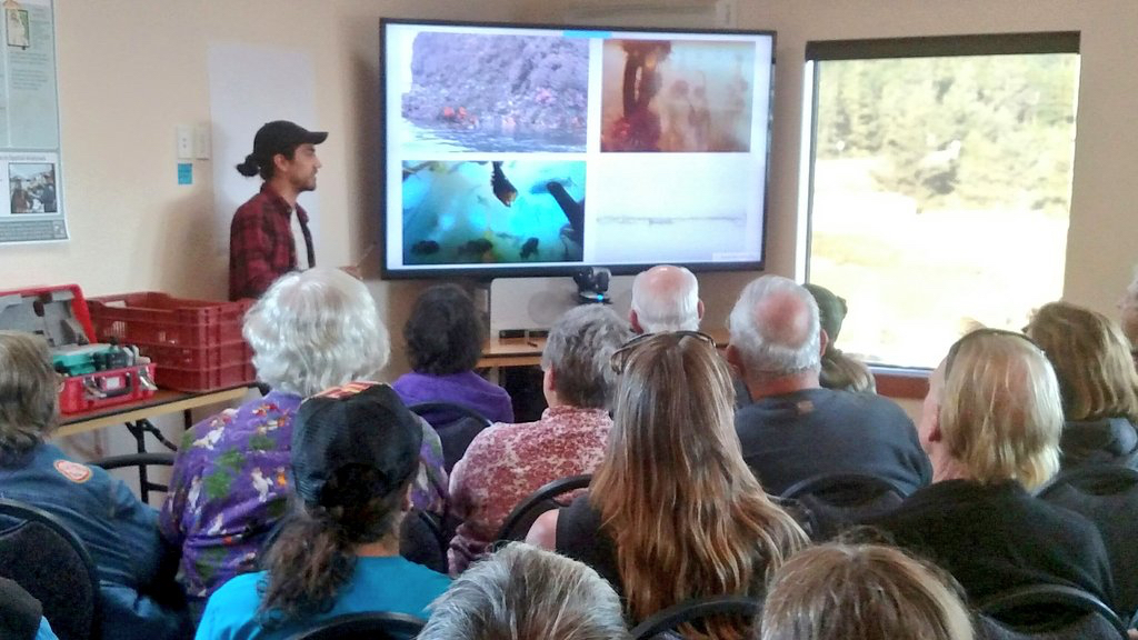
2018 team member Dylan presenting at the Port Orford community presentation. Source: T. Calvanese.
I think almost everyone in the scientific community would agree that outreach and engagement are important and that we should strive to interact frequently with the public to be transparent and build public trust, as well as to enable mutual learning. However, in my opinion, most scientists rarely put in the work needed to actually reach out to, and engage with, the community. Outreach and engagement have become buzzwords that are often thrown around, and with some hand-waving, can create the illusion that scientists are doing solid outreach and engagement work. For some, the words are probably even used interchangeably, which isn’t correct as they mean two different things.
Outreach and engagement should be thought of as occurring on two different ends of a spectrum. Outreach occurs in a one-way direction. Examples of outreach are public seminars delivered by a scientist (like Hatfield’s monthly Science on Tap) or fairs where the public is invited to come and talk to different scientific entities at their respective booths (like Hatfield’s annual Marine Science Day). Outreach is a way for scientists to disseminate their research to the public and often do not warrant the umbrella term engagement, as these “conversations” are not two-way. Engagement is collaborative and refers to intentional interactions where both sides (public and scientist) share and receive. It goes beyond a scientist telling the public about what they have been doing, but also requires the scientist to listen, absorb, and implement what the views from the ‘other side’ are.
2015 team tracking a whale on Graveyard Point above the port of Port Orford. Source: F. Sullivan.
Now that I have (hopefully) clarified the distinction between the two terms, I am going to shift the focus to specifically talk about the Port Orford project. Before I do, I would like to emphasize that I do not think our outreach and engagement is the be-all and end-all. There is definitely room for improvement and growth, but I do believe that we actively work hard to do both and to center these aspects within the project, rather than doing it as an afterthought to tick a box.
In talking about outreach and engagement, I have been using the words ‘public’ and ‘community’. I think these words conjure an image of a big group of people, an entire town, county, state or even nation. While this can be the case, it can also refer to smaller groups of people, even individuals. The outreach we conduct for the Port Orford project certainly occurs at the town-level. At the end of every field season, we give a community presentation where the field team and Leigh present new findings and give a recount of the field season. In the past, various teams have also given talks at the Humbug Mountain Campground and at Redfish Rocks Community Team events. These events, especially the community presentation, have been packed to the brim every year, which shows the community’s interest for the gray whales and our research. In fact, Tom Calvanese, the OSU Port Orford Field Station manager, has shared with me that now in early summer, Port Orford residents ask him when the ‘whale team’ is returning. I believe that our project has perhaps shifted the perception the local community has of scientists a little bit. Although in our first year or two of the project we may have been viewed as nosy outsiders, I feel that now we are almost honorary members within the community.
A packed room at the 2017 Port Orford community presentation. Photo: GEMM Lab.
Our outreach is not just isolated to one or two public talks per field season though. We have been close collaborators with South Coast Tours (SCT), an adventure tour company headed by Dave Lacey, since the start of the project. During the summer, SCT has almost daily kayak and fishing tours (this year, boat tours too!) out of Port Orford. The paddle routes of SCT and our kayak team will typically intersect in Tichenor’s Cove around mid-morning. When this happens, we form a little kayak fleet with the tour and research kayaks and our kayak team gives a short, informal talk about our research. We often pass around samples of zooplankton we just collected and answer questions that many of the paddlers have. These casual interactions are a highlight to the guests on SCT’s tours (Dave’s words, not mine) and they also provide an opportunity for the project’s interns to practice their science communication skills in a ‘low-stakes’ setting.
The nature of our engagement is more at the individual-level. Since the project’s conception in 2015, the team has been composed of some combination of 4-5 students, be it high school, undergraduate or graduate students. Aside from Florence Sullivan and myself as the GEMM Lab graduate student project leads, in total, we have had 16 students participate in the program, of which 4 were high school students (two from Port Orford’s Pacific High School and two from Astoria High School), 11 OSU and Lawrence University undergraduates, and 1 Duke University graduate student. This year we will be adding 3 more to the total tally (1 Pacific High School student, 1 OSU undergrad, and 1 graduate student from the Vrije Universiteit Brussel in Belgium). I am the first to admit that our yearly (and total) numbers of ‘impacted’ students is small. Limitations of funding and also general logistics of coordinating a large group of interns to participate in field work prevent us from having a larger cohort participate in the field season every summer. However, the impact on each of these students is huge.
The 2019 team with Dave Lacey who instructed our kayak paddle & safety course. Photo: L. Hildebrand.
If I had to pick one word to describe the 6-week Port Orford field season, it would be ‘intense’. The word is perfect because it can simultaneously describe something positive and negative, and the Port Orford field season definitely has elements of both. Both as a team and as individuals we experience incredible high points (an example being last year when we saw Port Orford’s favorite whale ‘Buttons’ breach multiple times on several different days), but we also have pretty low points (I’m thinking of a day in 2018 when two of my interns tried incredibly hard to get our GoPro stick dislodged from a rocky crevice for over 1-hour before radioing me to tell me they couldn’t retrieve it). These highs and lows occur on top of the team’s slowly depleting levels of energy as the field season goes on; with every day we get up at 5:30 am and we get a little more exhausted. The work requires a lot of brain power, a lot of muscle, and a lot of teamwork. Like I said, it’s intense and that’s coming from someone who had several years of marine mammal field work experience before running this project for the first time in 2018. The majority of the interns who have participated in our project have had no marine mammal field experience, some have had no field experience at all. It’s double, if not triple, intense for the interns!
I ask a lot of my interns. I am aware of that. It has been a steep learning curve for me since I took on the project in 2018. I’ve had to adjust my expectations and remember not to measure the performance of my interns against my own. I can always give 110% during the field season, even when I’m exhausted, because the stakes are high for me. After all, the data that is being collected feeds straight into my thesis. However, it took me a while to realize that the stakes, and therefore the motivation, aren’t the same for my interns as they are for me. And so, expecting them to perform at the same level I am, is unfair. I believe I have grown a lot since running that first field season. I have taken the feedback from interns to heart and tried to make adjustments accordingly. While those adjustments were hard because it ultimately meant making compromises that affected the amount of data collected, I recognize and respect the need to make those adjustments. I am incredibly grateful to all of the interns, including the ones that participated before my leadership of the project, who really gave it their all to collect the data that I now get to dig into and draw conclusions from.
2016 interns Kelli and Catherine paddling to a kayak sampling station. Photo: F. Sullivan.
But, as I said before, engagement is not one-sided, and I am not the only one who benefits from having interns participate in the project. The interns themselves learn a wealth of skills that are valuable for the future. Some of these skills are very STEM (Science, Technology, Engineering & Mathematics) specific (e.g. identifying zooplankton with a microscope, tracking whales with a theodolite), but a lot of them are transferrable to non-STEM futures (e.g. attention to detail and concentration required for identifying zooplankton, team work, effective communication). Our reach may be small with this project but the impact that participating in our internship has on each intern is a big one. Three of our four high school interns have gone on to start college. One plans to major in Marine Studies (in part a result of participating in this internship) while another decided to go to college to study Biology because of this internship. Several of the undergraduate students that participated in the 2015, 2016, 2017 & 2018 field seasons have gone on to start Master’s degrees at graduate schools around the country (3 of which have already graduated from their programs). A 2015 intern now teaches middle school in Washington and a 2016 intern is working with Oceans Initiative on their southern resident killer whale project this summer. Leigh, Florence and I have written many letters of recommendations for our interns, and these letters were not written out of duty, but out of conviction.
I love working closely with students and watching them grow. For the last two years, my proudest moment has always been watching my interns present our research at the annual community presentation we give at the end of the field season in Port Orford. No matter the amount of lows and struggles I experienced throughout the season, I watch my interns and my face almost hurts because of the huge smile on my face. The interns truly undergo a transformation where at the start of the season they are shy or feel inadequate and awkward when talking to the public about gray whales and the methods we employ to study them. But on that final day, there is so much confidence and eloquence with which the interns talk about their internship, that they are oftentimes even comfortable enough to crack jokes and share personal stories with the audience. As I said before, engagement of this nature is hard to measure and put a number on. Our statistic (engaging with 16 students) makes it sound like a small impact, but when you dig into what these engagements have meant for each student, the impact is enormous.
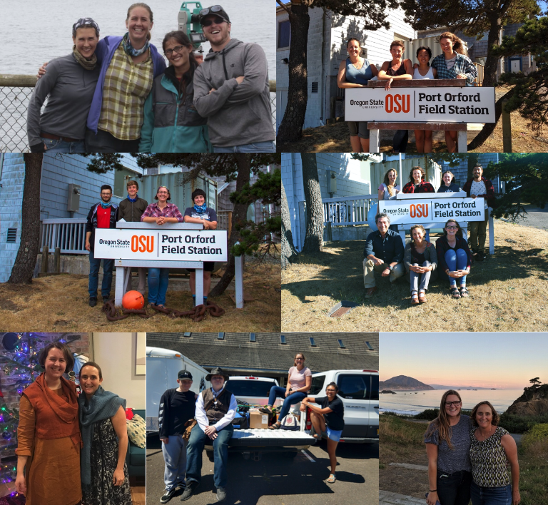
All of the past PO gray whale ecology teams, from left to right: 2015 (Sarah, Florence, Cricket, Justin), 2016 (Florence, Kelli, Catherine, Cathryn), 2017 (Nathan, Quince, Florence, Morgan), 2018 (Haley, Robyn, Hayleigh, Dylan, Lisa), and 2019 (Anthony, Donovan, Lisa, Mia). Bottom left: Florence and Leigh; bottom right: Lisa and Leigh.
I treasure my 6 weeks in Port Orford. Even though they are intense and there are new challenges every year, they bring me a lot of happiness. And it’s only in part because I get to see gray whales and kayak on an (almost) daily basis. A large part is because of the bonds I have formed and continue to cultivate with Port Orford locals, the leaps and bounds I know the interns will make, and the fact that the gray whales, completely unknowingly, bring together a small group of students and a community every year.
If you feel like taking a trip down memory lane, below are the links of the blogs written by previous PO interns:
Clara Bird, Masters Student, OSU Department of Fisheries and Wildlife, Geospatial Ecology of Marine Megafauna Lab
A big part of graduate school involves extensive reading to learn about the previous research conducted in the field you are joining and the embedded foundational theories. A firm understanding of this background literature is needed in order to establish where your research fits. Science is a constructive process; to advance our disciplines we must recognize and build upon previous work. Hence, I’ve been reading up on the central topic of my thesis: behavioral ecology. It is equally important to study the methods used in these studies as to understand the findings. As discussed in a previous blog, ethograms are a central component of the methodology for studying behavior. Ethograms are lists of defined behaviors that help us properly and consistently collect data in a standardized approach. It is especially important in a project that spans years to know that the data collected at the beginning was collected in the same way as the data collected at the end of the project.
While ethograms and standardized methods are commonly used within a study, I’ve noticed from reading through studies on cetaceans, a lack of standardization across studies. Not all behaviors that are named the same way have matching definitions, and not all behaviors with similar definitions have matching names. Of all the behaviors, “milling” may be the least standardized.
While milling is not in our ethogram (Leigh believes this term is a “cheat” for when behavior is actually “unknown”), we occasionally use “milling” in the field to describe when the gray whales are swimming around in an area, not foraging, but not in any other primary behavior state (travel, social, or rest). Sometimes we use when we think the whale may be searching, but we aren’t 100% sure yet. A recent conversation during a lab meeting on the confusing nature of the term “milling” inspired me to dig into the literature for this blog. I searched through the papers I’ve saved for my literature review and found 18 papers that used the term milling. It was fascinating to read how variably the term has been defined and used.
When milling was defined in these papers, it was most commonly described as numerous directional changes in movement within a restricted area 1–8. Milling often co-occurred with other behavior states. Five of these eight studies described milling as co-occurring with foraging behavior 3–6,8. In one case, milling was associated with foraging and slow movement 8. While another study described milling as passive, slow, nondirectional movement 9.
Eight studies used the term milling without defining the behavior 10–17. Of these, five described milling as being associated with other behavior states. Three studies described milling as co-occurring with foraging 10,14,16, one said that it co-occurred with social behavior 13, and another described milling as being associated with resting/slow movement 12.
In addition to this variety of definitions and behavior associations, there were also inconsistencies with the placement of “milling” within ethograms. In nine studies, milling was listed as a primary state 1,2,4,7–9,15,17,18. But, in two studies that mentioned milling and used an ethogram, milling was not included in the ethogram 6,14.
Diving into the associations between milling and foraging reveal how varied the use of milling has been within the cetacean literature. For example, two studies simply described milling as occurring near foraging in time 10,16. While another two studies explained that milling was applied in situations where there was evidence of feeding without feeding being directly observed 8,14. Bobkov et al. (2019) described milling as occurring between feeding cycles along with breathing. Lastly, two studies describe milling as a behavior within the foraging primary state 3,5, while another study described feeding as a behavior within milling 4.
It’s all rather confusing, huh? Across these studies, milling has been defined, mentioned without being defined, included in ethograms as a primary state, included in ethograms as a sub-behavior, and excluded from ethograms. Milling has also been associated with multiple primary behavior states (foraging, resting, and socializing). It has been described as both passive 9 and slow 12, and strong 16 and active 5.
It appears that milling is often used to describe behaviors that the observer cannot distinctly classify or describe its function. I have also struggled to define these times when a whale is in between behavior states; I often end up calling it “just being a whale”, which includes time spent breathing at the surface, or just swimming around.
As I’ve said above, Leigh thinks that this term is a “cheat” for when a behavior is actually “unknown”. I think we have trouble equating “milling” with “unknown” because it seems like “unknown” should refer to a behavior where we can’t quite tell what the whale is doing. However, during milling, we can see that the whale is swimming at the surface. But here’s the thing, while we can see what the whale is doing, the function of the behavior is still unknown. Instead of using an indistinct term, we should use a term that better describes the behavior. If it’s swimming at the surface, name the behavior “swimming at the surface”. If we can’t tell what the whale is doing because we can’t quite see what it’s doing, then name the behavior “unknown-partially visible”. Instead of using vague terminology, we should use clear names for behaviors and embrace using the term “unknown”.
I am most certainly not criticizing these studies as they all provided valuable contributions and interesting results. The studies that asked questions about behavioral ecology defined milling. The term was mentioned without being defined in studies focused on other topics. So, defining behaviors mentioned was less important.
With this exploration into the use of “milling” in studies, I am not implying that all behavioral ecologists need to agree on the use of the same behavior terms. However, I have learned clear definitions are critical. This lesson is also important outside of behavioral ecology. Different labs, and different people, use different terms for the same things. As I dig into my thesis, I am keeping a list of terminology I use and how I define those terms, because as I learn more, my terminology evolves and changes. For example, at the beginning of my thesis I used “sub-behavior” to refer to behaviors within the primary state categories. But, now after chatting with Leigh and learning more, I’ve decided to use the term “tactic” instead as these are often processes or events that contribute to the broader behavior state. My running list of terminology helps me remember what I meant when I used a certain word, so that when I read my notes from three months ago, I can know what I meant. Digging into the literature for this blog reminded me of the importance of clearly defining all terminology and never assuming that everyone uses the same term in the same way.
Check out these videos to see some of the behaviors we observe:
References
1. Mallonee, J. S. Behaviour of gray whales (Eschrichtius robustus) summering off the northern California coast, from Patrick’s Point to Crescent City. Can. J. Zool.69, 681–690 (1991).
2. Clarke, J. T., Moore, S. E. & Ljungblad, D. K. Observations on gray whale (Eschrichtius robustus) utilization patterns in the northeastern Chukchi Sea. Can. J. Zool67, (1988).
3. Ingram, S. N., Walshe, L., Johnston, D. & Rogan, E. Habitat partitioning and the influence of benthic topography and oceanography on the distribution of fin and minke whales in the Bay of Fundy, Canada. J. Mar. Biol. Assoc. United Kingdom87, 149–156 (2007).
4. Lomac-MacNair, K. & Smultea, M. A. Blue Whale (Balaenoptera musculus) Behavior and Group Dynamics as Observed from an Aircraft off Southern California. Anim. Behav. Cogn.3, 1–21 (2016).
5. Lusseau, D., Bain, D. E., Williams, R. & Smith, J. C. Vessel traffic disrupts the foraging behavior of southern resident killer whales Orcinus orca. Endanger. Species Res.6, 211–221 (2009).
6. Bobkov, A. V., Vladimirov, V. A. & Vertyankin, V. V. Some features of the bottom activity of gray whales (Eschrichtius robustus) off the northeastern coast of Sakhalin Island. 1, 46–58 (2019).
7. Howe, M. et al. Beluga, Delphinapterus leucas, ethogram: A tool for cook inlet beluga conservation? Mar. Fish. Rev.77, 32–40 (2015).
8. Clarke, J. T., Christman, C. L., Brower, A. A. & Ferguson, M. C. Distribution and Relative Abundance of Marine Mammals in the northeastern Chukchi and western Beaufort Seas, 2012. Annu. Report, OCS Study BOEM117, 96349–98115 (2013).
9. Barendse, J. & Best, P. B. Shore-based observations of seasonality, movements, and group behavior of southern right whales in a nonnursery area on the South African west coast. Mar. Mammal Sci.30, 1358–1382 (2014).
10. Le Boeuf, B. J., M., H. P.-C., R., J. U. & U., B. R. M. and F. O. High gray whale mortality and low recruitment in 1999: Potential causes and implications. (Eschrichtius robustus). J. Cetacean Res. Manag.2, 85–99 (2000).
11. Calambokidis, J. et al. Abundance, range and movements of a feeding aggregation of gray whales (Eschrictius robustus) from California to southeastern Alaska in 1998. J. Cetacean Res. Manag.4, 267–276 (2002).
12. Harvey, J. T. & Mate, B. R. Dive Characteristics and Movements of Radio-Tagged Gray Whales in San Ignacio Lagoon, Baja California Sur, Mexico. in The Gray Whale: Eschrichtius Robustus (eds. Jones, M. Lou, Folkens, P. A., Leatherwood, S. & Swartz, S. L.) 561–575 (Academic Press, 1984).
13. Lagerquist, B. A. et al. Feeding home ranges of pacific coast feeding group gray whales. J. Wildl. Manage.83, 925–937 (2019).
14. Barrett-Lennard, L. G., Matkin, C. O., Durban, J. W., Saulitis, E. L. & Ellifrit, D. Predation on gray whales and prolonged feeding on submerged carcasses by transient killer whales at Unimak Island, Alaska. Mar. Ecol. Prog. Ser.421, 229–241 (2011).
15. Luksenburg, J. A. Prevalence of External Injuries in Small Cetaceans in Aruban Waters, Southern Caribbean. PLoS One9, e88988 (2014).
16. Findlay, K. P. et al. Humpback whale “super-groups” – A novel low-latitude feeding behaviour of Southern Hemisphere humpback whales (Megaptera novaeangliae) in the Benguela Upwelling System. PLoS One12, e0172002 (2017).
17. Villegas-Amtmann, S., Schwarz, L. K., Gailey, G., Sychenko, O. & Costa, D. P. East or west: The energetic cost of being a gray whale and the consequence of losing energy to disturbance. Endanger. Species Res.34, 167–183 (2017).
18. Brower, A. A., Ferguson, M. C., Schonberg, S. V., Jewett, S. C. & Clarke, J. T. Gray whale distribution relative to benthic invertebrate biomass and abundance: Northeastern Chukchi Sea 2009–2012. Deep. Res. Part II Top. Stud. Oceanogr.144, 156–174 (2017).
Knowing what and how much prey a predator feeds on are key components to better understanding and conserving that predator. Prey abundance and availability are frequently predictors for marine predator reproductive success and population dynamics. It is the reason why the GEMM Lab makes a concerted effort to not only track our main taxa of interest (marine mammals) but to simultaneously measure their prey. However, over the last decade or two, there has been increased recognition that prey quality is also highly important in understanding a predator’s ecology (Spitz et al. 2012). Optimal foraging theory is a widely accepted framework that posits that predators should attempt to maximize energy gained and minimize energy spent during a foraging event (Charnov 1976, Krebs 1978, Pyke 1984). Thus, knowledge of how valuable a prey item is in terms of its energetic content is an important part of the equation when applying optimal foraging theory to a predator of interest.
Ideally, the prey species with the highest energetic value would also be the easiest, most ubiquitous and least energetically expensive prey item to capture and consume, such that a predator truly could expend very little energy to get very high energetic rewards. However, it rarely is this straightforward. The caloric content of several marine prey species has been shown to increase with increasing size (e.g. Benoit-Bird 2004; Fig. 1), both length and weight. Yet, increasing size often also means increased mobility and, as a result, ability to evade and escape predation. Furthermore, increasing size also inherently means decreasing abundances – there will always be billions more krill in the ocean than whales based solely on cost of reproduction. Therefore, just based on sheer numbers, there are fewer big prey items, which increases the time between, and decreases the likelihood of, a predator encountering big prey items. So, there are clear trade-offs here. It may take longer to locate and capture a high value prey item, which costs more energy to capture, but the payout could potentially be much bigger. However, if a predator gambles too much, then their net energy expenditure to obtain high value prey may be higher than the net energy gained. Instead, it may be worth pursuing smaller prey items with lower energetic values, where discovery and capture success are higher and more frequent. However, in this case, many, many more pursuits are likely needed, thus costing more energy to meet daily energetic demands.
Figure 1. Increasing caloric content with increasing length (a) and wet weight (b). Figures and caption reproduced from Benoit-Bird 2004.
Is your head spinning as much as mine? Let me try and simplify this complex web of interactions with a tangible example. Bowen et al. (2002) investigated foraging of harbor seals in Nova Scotia to assess prey profitability of different species. By attaching camera systems to the backs of 39 adult male harbor seals, the authors identified sand lance and flounder to be the most targeted prey species. However, there were significant differences in pursuit/handling cost per prey type (kJ/min) with sand lance only requiring 14.8 ± 2.7, whereas flounder required significantly more at 30.3 ± 7.9. Therefore, based solely on energy required to capture prey, the sand lance would seem to be the better option. In fact, to a certain degree, this hypothesis is actually true when we compare the energetic content of the two prey types. Sand lance have a higher energetic value at lengths of 10 and 15 cm (53.6 and 95.8 kJ, respectively) compared to flounder (22.6 and 88.6 kJ, respectively). So, the net gain of a harbor seal foraging on a 15 cm sand lance (assuming that it only takes 1 minute to catch the fish – this is more for explanatory purposes as it likely takes much longer for a harbor seal to capture a fish) would be 81 kJ. This gain is larger than that of a 15 cm flounder (58.3 kJ). However, once we compare these fish at 20 and 25 cm lengths, the flounder actually becomes the more beneficial prey item at 232.6 and 492.3 kJ, respectively, over the sand lance (158.1 and 233.8 kJ). Now, assuming once again that it only takes 1 minute to catch the fish, the harbor seal enjoys a net energetic gain of a whopping 462 kJ when capturing a 25 cm flounder compared to 219 kJ for a sand lance of the same size – that makes the flounder more than twice as profitable!
The Bowen et al. study is an excellent demonstration of the importance of considering the quality of prey items when studying the ecology of marine predators. However, the authors did not assess the relative availability of sand lance and flounder. Ideally, foraging ecology studies aimed at understanding prey choice would try to address both important prey metrics – quality and quantity. This goal is the exact aim of my second Master’s thesis chapter where I am investigating whether prey quality (determined through community composition and caloric content) or prey quantity (measured as relative density) is more important in driving fine-scale gray whale foraging behavior in Port Orford, Oregon (Fig. 2). This question can be simplified by asking does it matter more what prey is in an area, or how much prey there is in an area? Or we can relate it back to the title of this post by asking whether individual gray whales would rather attend a cheap all-you-can-eat buffet or an expensive fine-dining restaurant. I am unfortunately not quite done with my analyses yet (but I’m getting closer!) and therefore am not ready to answer these questions. However, I have done extensive research on this topic and therefore am in a position to briefly mention a few other studies that have investigated these questions for other marine predators.
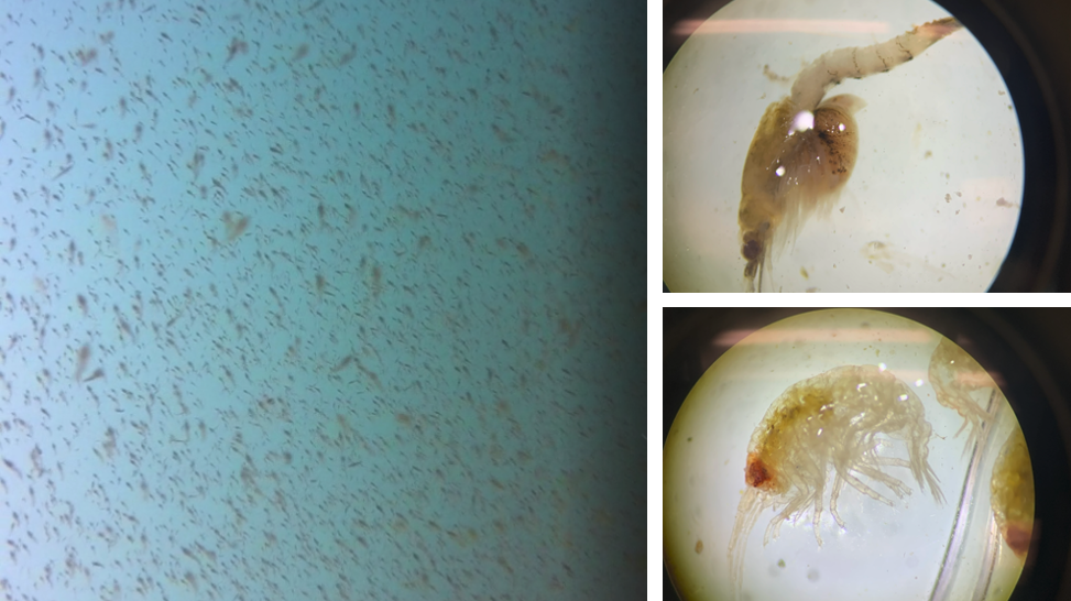
Figure 2. A question of what or how much. Left image: example of the screenshots we take to estimate relative prey density in Port Orford. Right images: two examples of the main prey species we find (top: mysid shrimp Neomysis rayii with a full brood pouch; bottom: amphipod Polycheria osborni).
Ludynia et al. (2010) explored reasons why African penguin (Spehniscus demersus) numbers have declined in Namibia. They found that after the collapse of pelagic fish stocks in the 1970s (including the principal penguin prey item, sardine), African penguins switched to feeding on bearded goby, which are considered a low-energy prey species. Bearded goby are relatively abundant along Namibia’s southern coast and as such, limited prey availability is not the reason for declining African penguin numbers. Therefore, the authors concluded that the low quality of bearded goby (compared to sardine) appears to be the reason for declining population trends of the penguins. This study demonstrates that African penguins do better when eating at a fine-dining restaurant, rather than loading up a whole plate of junk food.
Grémillet et al. (2004) studied the foraging effort and number of successful prey captures per foraging trip (yield) of great cormorants (Phalacrocorax carbo) in Greenland in relation to prey abundance and quality within their foraging areas. The authors radio-tracked 11 great cormorants during a total of 163 foraging trips to estimate foraging effort and yield. The study found that contrary to the authors’ hypothesis, great cormorants foraged in areas of low prey abundance where the average caloric value was also relatively low. Therefore, in this example, it would seem that the predator of interest prioritizes neither high quality nor quantity when foraging.
Haug et al. (2002) investigated the variations in minke whale (Balaenoptera acutorostrata) diet and body condition in response to ecosystem changes in the Barents Sea. The main prey item of minke whales in the Barents Sea is immature herring. However, when recruitment failure and subsequent weak cohorts leads to reduced availability of immature herring, minke whales switched their diet to other prey items such as krill, capelin, and sometimes other gadoid fish species. The authors found a correlation between body condition of minke whales and immature herring abundances, such that minke whales displayed a poor body condition during low immature herring abundances. However, in the years of low immature herring abundance, abundances of krill and capelin were not low. Therefore, similar to the Ludynia et al. (2010) study, it seems that minke whales in the Barents Sea also do better in years when the prey type of highest caloric value is the most abundant. However, decreases in high quality prey has not led to population declines in minke whales in the Barents Sea, indicating that they likely take advantage of high quantities of low quality prey, unlike the African penguins.
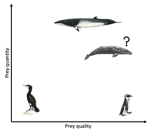
Clearly, the answer as to whether marine predators prefer quality over quantity is not simple and constant. Rather, prey preference varies based on predator needs and ecology, falling anywhere on a broad spectrum from low to high prey quality and low to high prey quantity (Fig. 3). To a certain extent, it probably also is not solely predator choice that determines what they eat but many other factors, such as climate, disturbance, and health. As a result, these preferences and choices will likely be fluid, rather than fixed. While I anticipate that individual gray whales will be flexible foragers, I do hypothesize that when there is a prey patch of a higher energetic value in the area, whales will preferentially consume these patches over areas where there is less energetically rich prey, even if it is more abundant.
Figure 3. A spectrum of prey quantity and quality. Giant cormorants forage on low prey quality & quantity (Grémillet et al. 2004). African penguin populations are declining despite high abundances of low quality prey, suggesting that high prey quality is important for their survival (Ludynia et al. 2010). Body condition of Barents Sea minke whales decreases when high quality prey is less abundant, however their populations have not declined, suggesting they instead exploit high abundances of low quality prey (Haug et al. 2002). What will the gray whales do?
Literature cited
Benoit-Bird, K. J. 2004. Prey caloric value and predator energy needs: foraging predictions for wild spinner dolphins. Marine Biology 145:435-444.
Bowen, W. D., D. Tuley, D. J. Boness, B. M. Bulheier, and G. J. Marshall. 2002. Prey-dependent foraging tactics and prey profitability in a marine mammal. Marine Ecology Progress Series 244:235-245.
Charnov, E. L. 1976. Optimal foraging, the marginal value theorem. Theoretical Population Biology 9(2):129-136.
Grémillet D., G. Kuntz, F. Delbart, M. Mellet, A. Kato, J-P. Robin, P-E. Chaillon, J-P. Gendner, S-H. Lorentsen, and Y. Le Maho. 2004. Linking the foraging performance of a marine predator to local prey abundance. Functional Ecology 18(6):793-801.
Haug, T., U. Lindstrøm, and K. T. Nilssen. 2002. Variations in minke whale (Balaenoptera acutorostrata) diet and body condition in response to ecosystem changes in the Barents Sea. Sarsia 87(6):409-422.
Krebs, J. R. 1978. Optimal foraging: decision rules for predators. Behvaioral Ecology: An Evolutionary Approach, eds. Krebs, J. R., and N. B. Davies. Oxford: Blackwell.
Ludynia, J., J-P. Roux, R. Jones, J. Kemper, and L. G. Underhill. 2010. Surviving off junk: low-energy prey dominates the diet of African penguins Spheniscus demersus at Mercury Island, Namibia, between 1996 and 2009. African Journal of Marine Science 32(3):563-572.
Pyke, G. H. 1984. Optimal foraging theory: a critical review. Annual Reviews of Ecology and Systematics 15:523-575.
Spitz, J., A. W. Trites, V. Becquet, A. Brind’Amour, Y. Cherel, R. Galois, and V. Ridoux. 2012. Cost of living dictates what whales, dolphins and porpoises eat: the importance of prey quality on predator foraging strategies. PLoS ONE 7(11):e50096.
Young, J. K., B. A. Black, J. T. Clarke, S. V. Schonberg, and K. H. Dunton. 2017. Abundance, biomass and caloric content of Chukchi Sea bivalves and association with Pacific walrus (Odobenus rosmarus divergens) relative density and distribution in the northeastern Chukchi Sea. Deep-Sea Research Part II 144:125-141.
Clara Bird, Masters Student, OSU Department of Fisheries and Wildlife, Geospatial Ecology of Marine Megafauna Lab
The GEMM Lab gray whale team is in the midst of preparing for our fifth field season studying the Pacific Coast Foraging Group (PCFG): whales that forage off the coast of Newport, OR, USA each summer. On any given good weather day from June to October, our team is out on the water in a small zodiac looking for gray whales (Figure 1). When we find a gray whale, we try to collect photo ID data, fecal samples, drone data, and behavioral data. We use the drone data to study both the whale’s body condition and their behavior. In a previous blog, I described ethograms and how I would like to use the behavior data from drone videos to classify behaviors, with the ultimate goal of understanding how gray whale behavior varies across space, time, and by individual. However, this explanation of studying whale behavior is actually a bit incomplete. Before we start fieldwork, we first need to decide how to collect that data.
Figure 1. Image of GEMM lab team collecting gray whale UAS data. Image taken under NOAA/NMFS permit #16111
As observers, we are far from omnipresent and there is no way to know what the animals are doing all of the time. In any environment, scientists have to decide when and where to observe their animals and what behaviors they are interested in recording. In many studies, behavior is recorded live by an observer. In those studies, other limitations need to be taken into account, such as human error and observer fatigue. Collecting behavioral data is particularly challenging in the marine environment. Cetaceans spend most of their lives out of sight from humans, their time at the surface is brief, and when they appear together in large groups it can be very difficult to keep track of who is doing what when. Imagine being in a boat trying to keep track of what three different whales are doing without a pre-determined method – the task could quickly become overwhelming and biased. This is why we need a methodology for collecting and classifying behavior. We cannot study behavior without acknowledging these limitations and the potential biases that come with the methods we choose. Different data collection methods are better suited to address different questions.
The use of drones gives us the ability to record cetacean behavior non-invasively, from a perspective that allows greater observation (Figure 2, Torres et al. 2018), and for later review, which is a significant improvement. However, as we prepare to collect more behavior data, we need to study the methods and understand the benefits and disadvantages of each approach so that we capture the information we need without bias. Altmann (1974) provides a thorough overview of behavioral sampling methods.
Figure 2. Diagram illustrating “whale surface time” relative to “whale visible time” data as collected from an unmanned aerial systems (UAS) aircraft flying over a gray whale as it moves sequentially (from right to left) from “headstand” foraging to surfacing. Figure from Torres et al. (2018).
Ad libitum behavioral sampling has no structure and occurs when we find a group of whales and just write down everything they are doing. This method is a good first step, however it comes with bias. Without structure, we cannot be sure that there was an equal probability of detecting each kind of behavior; this problem is called detectability bias. This type of bias is an issue if we are trying to answer questions about how often a behavior occurs, or what percent of time is spent in each behavior state. This is a bias to be especially concerned about when it comes to cetaceans because there are many examples of behaviors with different levels of detectability. An extreme example would be the detectability of breaching versus a behavior that takes place under the surface. A breaching whale is easier to spot and more exciting, which could lead to results suggesting that whales breach more often than they do relative to underwater behaviors. While it’s impossible to eliminate detectability bias, other sampling methods employ decision rules to try and reduce its effect. Many decision rules revolve around time, such as setting a minimum or maximum observation time interval. Other time rules involve recording the behavior state at set intervals of time (e.g., every 5 minutes). Setting observation boundaries helps standardize the methods and the data being collected.
In a structured sampling plan, the first big decision that needs to be addressed is the need to know the duration of behaviors. Point events do not include duration data but can be used to study the frequencies of behaviors. For example, if my research question was “Do whales perform “headstands” in a specific habitat type?”, then I would need point events of headstanding behavior. But, if I wanted to ask, “Do whales spend more time spent headstanding in a specific habitat type than in other habitat types?”, I would need headstanding to be a state event. State events are events with associated duration information and can be used for activity budgets. Activity budgets show how much time an animal spends in each behavior state. Some sampling methods focus on collecting only point events. However, to get the most complete understanding of behavior I think it’s important to collect both. Focal animal follows are another method of collecting more detailed data and is commonly used in cetacean studies.
The explanation of a focal follow method is in the name. We focus on one individual, follow it, and record all of its behaviors. When employing this method, decisions are made about how an individual is chosen and how long it is followed. In some cases, the behavior of this animal is used as a proxy for the behavior of an entire group. I essentially use the focal follow method in my research. While I review drone footage to record behavioral data instead of recording behaviors live in the field, I focus on one individual a time as I go through the videos. To do this I use a software called BORIS (Friard and Gamba 2016) to mark the time of each behavior per individual (Figure 3). If there are three individuals in a video, I’ll review the footage three times to record behaviors once per individual, focusing on each in turn.
Figure 3. Screenshot of BORIS layout.
While the drone footage brings the advantages of time to review and a better view of the whale, we are constrained by the duration of a flight. Focal follows would ideally last longer than the ~15 minutes of battery life per drone flight. Our previously collected footage gives us snapshots of behavior, and this makes it challenging to compare and analyze durations of behaviors. Therefore, I am excited that we are going to try conducting drone focal follows this summer by swapping out drones when power runs low to achieve longer periods of video coverage of whale behavior. I’ll be able to use these data to move from snapshots to analyzing longer clips and better understanding the behavioral ecology of gray whales. As exciting as this opportunity is, it also presents the challenge of method development. So, I now need to develop decision rules and data collection methods to answer the questions that I have been eagerly asking.
Friard, Olivier, and Marco Gamba. 2016. “BORIS: A Free, Versatile Open-Source Event-Logging Software for Video/Audio Coding and Live Observations.” Methods in Ecology and Evolution 7 (11): 1325–30. https://doi.org/10.1111/2041-210X.12584.
Torres, Leigh G., Sharon L. Nieukirk, Leila Lemos, and Todd E. Chandler. 2018. “Drone up! Quantifying Whale Behavior from a New Perspective Improves Observational Capacity.” Frontiers in Marine Science 5 (SEP). https://doi.org/10.3389/fmars.2018.00319.
The last two months have been challenging for everyone across the world. While I have also experienced lows and disappointments during this time, I always try to see the positives and to appreciate the good things every day, even if they are small. One thing that I have been extremely grateful and excited about every week is when the clock strikes 9:58 am every Thursday. At that time, I click a Zoom link and after a few seconds of waiting, I am greeted by the smiling faces of the GEMM Lab. This spring term, our Principal Investigator Dr. Leigh Torres is teaching a reading and conference class entitled ‘Cetacean Behavioral Ecology’. Every week there are 2-3 readings (a mix of book chapters and scientific papers) focused on a particular aspect of behavioral ecology in cetaceans. During the first week we took a deep dive into the foundations of behavioral ecology (much of which is terrestrial-based) and we have now transitioned into applying the theories to more cetacean-centric literature, with a different branch of behavior and ecology addressed each week.
Leigh dedicated four weeks of the class to discussing foraging behavior, which is particularly relevant (and exciting) to me since my Master’s thesis focuses on the fine-scale foraging ecology of gray whales. Trying to understand the foraging behavior of cetaceans is not an easy feat since there are so many variables that influence the decisions made by an individual on where and when to forage, and what to forage on. While we can attempt to measure these variables (e.g., prey, environment, disturbance, competition, an individual’s health), it is almost impossible to quantify all of them at the same time while also tracking the behavior of the individual of interest. Time, money, and unworkable weather conditions are the typical culprits of making such work difficult. However, on top of these barriers is the added complication of scale. We still know so little about the scales at which cetaceans operate on, or, more importantly, the scales at which the aforementioned variables have an effect on and drive the behavior of cetaceans. For instance, does it matter if a predator is 10 km away, or just when it is 1 km away? Is a whale able to sense a patch of prey 100 m away, or just 10 m away? The same questions can be asked in terms of temporal scale too.
What is that gray whale doing in the kelp? Source: F. Sullivan.
As such, cetacean field work will always involve some compromise in data collection between these factors. A project might address cetacean movements across large swaths of the ocean (e.g., the entire U.S. west coast) to locate foraging hotspots, but it would be logistically complicated to simultaneously collect data on prey distribution and abundance, disturbance and competitors across this same scale at the same time. Alternatively, a project could focus on a small, fixed area, making simultaneous measurements of multiple variables more feasible, but this means that only individuals using the study area are studied. My field work in Port Orford falls into the latter category. The project is unique in that we have high-resolution data on prey (zooplankton) and predators (gray whales), and that these datasets have high spatial and temporal overlap (collected at nearly the same time and place). However, once a whale leaves the study area, I do not know where it goes and what it does once it leaves. As I said, it is a game of compromises and trade-offs.
Ironically, the species and systems that we study also live a life of compromises and trade-offs. In one of this week’s readings, Mridula Srinivasan very eloquently starts her chapter entitled ‘Predator/Prey Decisions and the Ecology of Fear’ in Bernd Würsig’s ‘Ethology and Behavioral Ecology of Odontocetes’ with the following two sentences: “Animal behaviors are governed by the intrinsic need to survive and reproduce. Even when sophisticated predators and prey are involved, these tenets of behavioral ecology hold.”. Every day, animals must walk the tightrope of finding and consuming enough food to survive and ensure a level of fitness required to reproduce, while concurrently making sure that they do not fall prey to a predator themselves. Krebs & Davies (2012) very ingeniously use the idea of economic analysis of costs and benefits to understand foraging behavior (but also behavior in general). While foraging, individuals not only have to assess potential risk (Fig. 1) but also decide whether a certain prey patch or item is profitable enough to invest energy into obtaining it (Fig. 2).
Leigh’s class has been great, not only to learn about foundational theories but to then also apply them to each of our study species and systems. It has been exciting to construct hypotheses based on the readings and then dissect them as a group. As an example, Sih’s 1984 paper on the behavioral response race of predators and prey prompted a discussion on responses of predators and prey to one another and how this affects their spatial distributions. Sih posits that since predators target areas with high prey densities, and prey will therefore avoid areas that predators frequent, their responses are in conflict with one another. Resultantly, there will be different outcomes depending on whichever response dominates. If the predator’s response dominates (i.e. predators are able to seek out areas of high prey density before prey can respond), then predators and prey will have positively correlated spatial distributions. However, if the prey responses dominate, then the spatial distributions of the two should be negatively correlated, as predators will essentially always be ‘one step behind’ the prey. Movement is most often the determinant factor to describe the strength of these relationships.
Video 1. Zooplankton closest to the camera will jump or dart away from it. Source: GEMM Lab.
So, let us think about this for gray whales and their zooplankton prey. The latter are relatively immobile. Even though they dart around in the water column (I have seen them ‘jump’ away from the GoPro when we lower it from the kayak on several occasions; Video 1), they do not have the ability to maneuver away fast or far enough to evade a gray whale predator moving much faster. As such, the predator response will most likely always be the strongest since gray whales operate at a scale that is several orders of magnitude greater than the zooplankton. However, the zooplankton may not be as helpless as I have made them seem. Based on our field observations, it seems that zooplankton often aggregate beneath or around kelp. This behavior could potentially be an attempt to evade predators as the kelp and reef crevices may serve as a refuge. So, in areas with a lot of refuges, the prey response may in fact dominate the relationship between gray whales and zooplankton. This example demonstrates the importance of habitat in shaping predator-prey interactions and behavior. However, we have often observed gray whales perform “bubble blasts” in or near kelp (Video 2). We hypothesize that this behavior could be a foraging tactic to tip the see-saw of predator-prey response strength back into their favor. If this is the case, then I would imagine that gray whales must decide whether the energetic benefit of eating zooplankton hidden in kelp refuges outweighs the energy required to pursue them (Fig. 2). On top of all these choices, are the potential risks and threats of boat traffic, fishing gear, noise, and potential killer whale predation (Fig. 1). Bringing us back to the analogy of economic analysis of costs and benefits to predator-prey relationships. I never realized it so clearly before, but gray whales sure do have a lot of decisions to make in a day!
Video 2. Drone footage of a gray whale foraging in kelp and performing a “bubble blast” at 00:40. Footage captured under NMFS permit #21678. Source: GEMM Lab.
Trying to tease apart these nuanced dynamics is not easy when I am unable to simply ask my study subjects (gray whales) why they decided to abandon a patch of zooplankton (Were the zooplankton too hard to obtain because they sought refuge in kelp, or was the patch unprofitable because there were too few or the wrong kind of zooplankton?). Or, why do gray whales in Oregon risk foraging in such nearshore coastal reefs where there is high boat traffic (Does their need for food near the reefs outweigh this risk, or do they not perceive the boats as a risk?). So, instead, we must set up specific hypotheses and use these to construct a thought-out and informed study design to best answer our questions (Mann 2000). For the past few weeks, I have spent a lot of time familiarizing myself with spatial packages and functions in R to start investigating the relationships between zooplankton and kelp hidden in the data we have collected over 4 years, to ultimately relate these patterns to gray whale foraging. I still have a long and steep journey before I reach the peak but once I do, I hope to have answers to some of the questions that the Cetacean Behavioral Ecology class has inspired.
Literature cited
Krebs, J. R., and N. B. Davies. 2012. Economic decisions and the individual in Davies, N. B. et al., eds. An introduction to behavioral ecology. John Wiley & Sons, Oxford.
Mann, J. 2000. Unraveling the dynamics of social life: long-term studies and observational methods in Mann, J., ed. Cetacean societies: field studies of dolphins and whales. University of Chicago Press, Chicago.
Sih, A. 1984. The behavioral response race between predator and prey. The American Naturalist 123:143-150.
Srinivasan, M. 2019. Predator/prey decisions and the ecology of fear in Würsig, B., ed. Ethology and ecology of odontocetes. Springer Nature, Switzerland.
Clara Bird, Masters Student, OSU Department of Fisheries and Wildlife, Geospatial Ecology of Marine Megafauna Lab
Whale blow, the puff of air mixed with moisture that a whale releases when it comes to the surface, is a famously thrilling indicator of the presence of a whale. From shore, spotting whale blow brings the excitement of knowing that there are whales nearby. During boat-based field work, seeing or hearing blow brings the rush of adrenaline meaning that it’s game time. Whale blow can also be used to identify different species of whales, for example gray whale blow is heart shaped (Figure 1). However, whale blow can be used for more than just spotting and identifying whales. We can use the time between blows to study energetics.
Figure 1. Gray whale blow is often heart shaped (when there is very little wind). Source: https://www.lajollalight.com/sdljl-natural-la-jolla-winter-wildlife-2015jan08-story.html
A blow interval is the time between consecutive blows when a whale is at the surface (Stelle, Megill, and Kinzel 2008). These are also known as short breath holds, whereas long breath holds are times between surfacings (Sumich 1983). Sumich (1983) hypothesized that short breath holds lead to efficient rates of oxygen use. The body uses oxygen to create energy, so “efficient rate of oxygen use” means that longer breath holds do not use much more oxygen and subsequently do not produce more energy. Surfacings, during which short blow intervals occur, are often thought of as recovery periods for whales. Think of it this way, when you sprint, immediately afterwards you typically need to take a break to just breathe and recover.
We hypothesize that we can use blow intervals as a measure of how strenuous an activity is; shorter blow intervals may indicate that an activity is more energetically demanding (Wursig, Wells, and Croll 1986). Let’s go back to the sprinting analogy and compare the energetic demands of walking and running. Imagine I asked you to walk for five minutes, stop and measure the time between each breath, and then run for five minutes and do the same; after running, you would likely breathe more heavily and take more breaths with less time between them. This result indicates that running is more demanding, which we already know because we can do other experiments with humans to study metabolic rate and related metrics. In the case of gray whales, we cannot do experiments in the same way, but we can use the same analogy. Several studies have examined how blow intervals differ between travelling and foraging.
Wursig, Wells, and Croll (1986) measured blow interval, surfacing time, and estimated dive depth and duration of gray whales in Alaska from a boat during the foraging season. They found that blow intervals were shorter during feeding. They also found that the number of blows per surfacing increased with increasing depth. Overall these findings suggest that during the foraging season, feeding is more strenuous than other behaviors and that deeper dives may be more physiologically stressful.
Stelle, Megill, and Kinzel (2008) studied gray whales foraging off of British Columbia, Canada. They found shorter blow intervals during foraging, intermediate blow intervals during searching, and longer blow intervals during travelling. Interestingly, within feeding behaviors, they found a difference between whales feeding on mysids (krill-like animals that swim in the water column) and whales feeding benthically on amphipods. They found that whales feeding on mysids made more frequent but shorter dives with short blow intervals at surface, while whales feeding benthically had longer dives with longer blow intervals. They hypothesized that this difference in surfacing pattern is because mysids might scatter when disturbed, so gray whales surface more often to allow the mysids swarm to reform. These studies inspired me to start investigating these same questions with my drone video data.
As I review the drone footage and code the behaviors I also mark the time of each blow. I’ve done some initial video coding and using this data I have started to look into differences in blow intervals. As it turns out, we see a similar difference in blow interval relative to behavior state in our data: whales that are foraging have shorter blow intervals than when traveling (Figure 2). It is encouraging to see that our data shows similar patterns.
Figure 2. Boxplot of mean blow interval per sighting of foraging whales and travelling whales.
Next, I would like to examine how blow intervals differ between foraging tactics. A significant part of my thesis is dedicated to studying specific foraging tactics. The perspective from the drone allows us to identify behaviors in greater detail than studies from shore or boat (Torres et al. 2018), allowing us to dig into the differences between the different foraging behaviors. The purpose of foraging is to gain energy. However, this gain is a net gain. To understand the different energetic “values” of each tactic we need to understand the cost of each behavior, i.e. how much energy is required to perform the behavior. Given previous studies, maybe blow intervals could help us measure this cost or at least compare the energetic demands of the behaviors relative to each other. Furthermore, because different behaviors are likely associated with different prey types (Dunham and Duffus 2001), we also need to understand the different energetic gains of each prey type (this is something that Lisa is studying right now, check out the COZI project to learn more). By understanding both of these components – the gains and costs – we can understand the energetic tradeoffs of the different foraging tactics.
Another interesting component to this energetic balance is a whale’s health and body condition. If a whale is in poor health, can it afford the energetic costs of certain behaviors? If whales in poor body condition engage in different behavior patterns than whales in good body condition, are these patterns explained by the energetic costs of the different foraging behaviors? All together this line of investigation is leading to an understanding of why a whale may choose to use different foraging behaviors in different situations. We may never get the full picture; however, I find it really exciting that something as simple and non-invasive as measuring the time between breaths can contribute such a valuable data stream to this project.
References
Dunham, Jason S., and David A. Duffus. 2001. “Foraging Patterns of Gray Whales in Central Clayoquot Sound, British Columbia, Canada.” Marine Ecology Progress Series 223 (November): 299–310. https://doi.org/10.3354/meps223299.
Stelle, Lei Lani, William M. Megill, and Michelle R. Kinzel. 2008. “Activity Budget and Diving Behavior of Gray Whales (Eschrichtius Robustus) in Feeding Grounds off Coastal British Columbia.” Marine Mammal Science 24 (3): 462–78. https://doi.org/10.1111/j.1748-7692.2008.00205.x.
Sumich, James L. 1983. “Swimming Velocities, Breathing Patterns, and Estimated Costs of Locomotion in Migrating Gray Whales, Eschrichtius Robustus.” Canadian Journal of Zoology 61 (3): 647–52. https://doi.org/10.1139/z83-086.
Torres, Leigh G., Sharon L. Nieukirk, Leila Lemos, and Todd E. Chandler. 2018. “Drone up! Quantifying Whale Behavior from a New Perspective Improves Observational Capacity.” Frontiers in Marine Science 5 (SEP). https://doi.org/10.3389/fmars.2018.00319.
Wursig, B., R. S. Wells, and D. A. Croll. 1986. “Behavior of Gray Whales Summering near St. Lawrence Island, Bering Sea.” Canadian Journal of Zoology 64 (3): 611–21. https://doi.org/10.1139/z86-091.