Fashionably late: New GEMM Lab publication measures lags between wind, upwelling, and blue whale occurrence

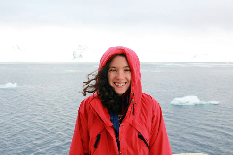
By Dawn Barlow, PhD Candidate, OSU Department of Fisheries and Wildlife, Geospatial Ecology of Marine Megafauna Lab

To understand the complex dynamics of an ecosystem, we need to examine how physical forcing drives biological response, and how organisms interact with their environment and one another. The largest animal on the planet relies on the wind. Throughout the world, blue whales feed areas where winds bring cold water to the surface and spur productivity—a process known as upwelling. In New Zealand’s South Taranaki Bight region (STB), westerly winds instigate a plume of cold, nutrient-rich waters that support aggregations of krill, and ultimately lead to foraging opportunities for blue whales. This pathway, beginning with wind input and culminating in blue whale occurrence, does not take place instantaneously, however. Along each link in this chain of events, there is some lag time.

Figure 1. A blue whale comes up for air in New Zealand’s South Taranaki Bight. Photo: L. Torres.

Our recent paper published in Scientific Reports examines the lags between wind, upwelling, and blue whale occurrence patterns. While marine ecologists have long acknowledged that lag plays a role in what drives species distribution patterns, lags are rarely measured, tested, and incorporated into studies of marine predators such as whales. Understanding lags has the potential to greatly improve our ability to predict when and where animals will be under variable environmental conditions. In our study, we used timeseries analysis to quantify lag between different metrics (wind speed, sea surface temperature, blue whale vocalizations) at different locations. While our methods are developed and implemented for the STB ecosystem, they are transferable to other upwelling systems to inform, assess, and improve predictions of marine predator distributions by incorporating lag into our understanding of dynamic marine ecosystems.

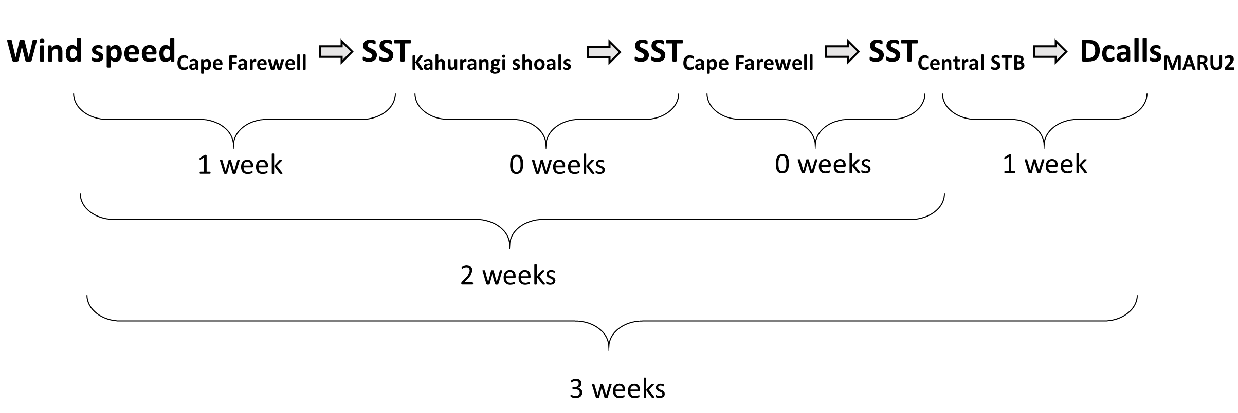
So, what did we find? It all starts with the wind. Wind instigates upwelling over an area off the northwest coast of the South Island of New Zealand called Kahurangi Shoals. This wind forcing spurs upwelling, leading to the formation of a cold water plume that propagates into the STB region, between the North and South Islands, with a lag of 1-2 weeks. Finally, we measured the density of blue whale vocalizations—sounds known as D calls, which are produced in a social context, and associated with foraging behavior—recorded at a hydrophone downstream along the upwelling plume’s path. D call density increased 3 weeks after increased wind speeds near the upwelling source. Furthermore, we looked at the lag time between wind events and aggregations in blue whale sightings. Blue whale aggregations followed wind events with a mean lag of 2.09 ± 0.43 weeks, which fits within our findings from the timeseries analysis. However, lag time between wind and whales is variable. Sometimes it takes many weeks following a wind event for an aggregation to form, other times mere days. The variability in lag can be explained by the amount of prior wind input in the system. If it has recently been windy, the water column is more likely to already be well-mixed and productive, and so whale aggregations will follow wind events with a shorter lag time than if there has been a long period without wind and the water column is stratified.

Figure 2. Top panel: Map of the study region within the South Taranaki Bight (STB) of New Zealand, with location denoted by the white rectangle on inset map in the upper right panel. All spatial sampling locations for sea surface temperature implemented in our timeseries analyses are denoted by the boxes, with the four focal boxes shown in white that represent the typical path of the upwelling plume originating off Kahurangi shoals and moving north and east into the STB. The purple triangle represents the Farewell Spit weather station where wind measurements were acquired. The location of the focal hydrophone (MARU2) where blue whale D calls were recorded is shown by the green star. (Reproduced from Barlow et al. 2021). Bottom panel: Results of the timeseries cross-correlation analyses, illustrating the lag between some of the metrics and locations examined.

This publication forms the second chapter of my PhD dissertation. However, in reality it is the culmination of a team effort. Just as whale aggregations lag wind events, publications lag years of hard work. The GEMM Lab has been studying New Zealand blue whales since Leigh first hypothesized that the STB was an undocumented foraging ground in 2013. I was fortunate enough to join the research effort in 2016, first as a Masters student and now as a PhD Candidate. I remember standing on the flying bridge of R/V Star Keys in New Zealand in 2017, when early in our field season we saw very few blue whales. Leigh and I were discussing this, with some frustration. Exclamations of “This is cold, upwelled water! Where are the whales?!” were followed by musings of “There must be a lag… It has to take some time for the whales to respond.” In summer 2019, Christina Garvey came to the GEMM Lab as an intern through the NSF Research Experience for Undergraduates program. She did an outstanding job of wrangling remote sensing and blue whale sighting data, and together we took on learning and understanding timeseries analysis to quantify lag. In a meeting with my PhD committee last spring where I presented preliminary results, Holger Klinck chimed in with “These results are interesting, but why haven’t you incorporated the acoustic data? That is a whale timeseries right there and would really add to your analysis”. Dimitri Ponirakis expertly computed the detection area of our hydrophone so we could adequately estimate the density of blue whale calls. Piecing everything together, and with advice and feedback from my PhD committee and many others, we now have a compelling and quantitative understanding of the upwelling dynamics in the STB ecosystem, and have thoroughly described the pathway from wind to whales in the region.

Figure 3. Dawn and Leigh on the flying bridge of R/V Star Keys on a windy day in New Zealand during the 2017 field season. Photo: T. Chandler.

Our findings are exciting, and perhaps even more exciting are the implications. Understanding the typical patterns that follow a wind event and how the upwelling plume propagates enables us to anticipate what will happen one, two, or up to three weeks in the future based on current conditions. These spatial and temporal lags between wind, upwelling, productivity, and blue whale foraging opportunities can be harnessed to generate informed forecasts of blue whale distribution in the region. I am thrilled to see this work in print, and equally thrilled to build on these findings to predict blue whale occurrence patterns.

Reference: Barlow, D.R., Klinck, H., Ponirakis, D., Garvey, C., Torres, L.G. Temporal and spatial lags between wind, coastal upwelling, and blue whale occurrence. Sci Rep 11, 6915 (2021). https://doi.org/10.1038/s41598-021-86403-y

The ecologist and the economist: Exploring parallels between disciplines

By Dawn Barlow1 and Johanna Rayl2

1PhD Candidate, Oregon State University Department of Fisheries and Wildlife, Geospatial Ecology of Marine Megafauna Lab

2PhD Student, Northwestern University Department of Economics

The Greek word “oikos” refers to the household and serves as the root of the words ecology and economics. Although perhaps surprising, the common origin reflects a shared set of basic questions and some shared theoretical foundations related to the study of how lifeforms on earth use scarce resources and find equilibrium in their respective “households”. Early ecological and economic theoretical texts drew inspiration from one another in many instances. Paul Samuelson, fondly referred to as “the father of modern economics,” observed in his defining work Foundations of Economic Analysis that the moving equilibrium in a market with supply and demand is “essentially identical with the moving equilibrium of a biological or chemical system undergoing slow change.” Likewise, early theoretical ecologists recognized the strength of drawing on theories previously established in economics (Real et al. 1991). Similar broad questions are central to researchers in both fields; in a large and dynamic system (termed “macro” in economics) scale, ecologists and economists alike work to understand where competitive forces find equilibrium, and an in individual (or micro) scale, they ask how individuals make behavior choices to maximize success given constraints like time, energy, wealth, or physical resources.

The central model economists have in mind when trying to understand human choices involves “constrained optimization”: what decision will maximize a person, family, firm, or other agent’s objectives given their limitations? For example, someone that enjoys relaxing but also seeks a livable income must choose how much time to devote to working versus relaxing, given the constraint of having just 24 hours in the day, and given the wage they receive from working. An economist studying this decision may want to learn about how changes in the wage will affect that person’s choice of working hours, or how much they dislike working relative to relaxing. Along similar lines, early ecologists theorized that organisms could be selected for one of two optimization strategies: minimizing the time spent acquiring a given amount of energy (i.e., calories from food), or maximizing total energy acquisition per unit of time (Real et al. 1991). Foundational work in the field of economics clarified numerous technical details about formulating and solving such optimization problems. Returning to the example of the leisure time decision, economic theory asks: does it matter if we model this decision as maximizing income given wages and limited time, or as minimizing hours spent working given a desired lifetime income?; can we formulate a “utility function” that  describes how well-off someone is with a given income and amount of leisure?; can we solve for the optimal amount of leisure with pen and paper? The toolkit arising from this work serves as a jumping off point for all contemporary economic research, and the kinds of choices understood under this framework is vast, from, where should a child attend school?; to, how should a government allocate its budget across public resources?

Early work in ecology drew from foundational concepts in economics, following the realization that the strategies by which organisms exploit resources most efficiently also involve optimization. This parallel was articulated by MacArthur and Pianka in their foundational 1966 paper Optimal Use of a Patchy Environment, in which they state: “In this paper we undertake to determine in which patches a species would feed and which items would form its diet if the species acted in the most economical fashion. Hopefully, natural selection will often have achieved such optimal allocation of time and energy expenditures.” Subsequently, this idea was refined into what is known in ecology as the marginal value theorem, which states that an animal should remain in a prey patch until the rate of energy gain drops below the expected energy gain in all remaining available patches (Charnov 1976). In other words, if it is more profitable to switch prey patches than to stay, an animal should move on. These optimization models therefore allow ecologists to pose specific evolutionary and behavioral hypotheses, such as examining energy acquisition over time to understand selective forces on foraging behavior.

As the largest animals on the planet, blue whales have massive prey requirements to meet energy demands. However, they must balance their need to feed with costs such as oxygen consumption during breath-holding, the travel time it takes to reach prey patches at depth, the physiological constraints of diving, and the necessary recuperation time at the surface. It has been demonstrated that blue whales forage selectively to optimize this energetic budget. Therefore, blue whales should only feed on krill aggregations when the energetic gain outweighs the cost (Fig. 1), and this pattern has been empirically demonstrated for blue whale populations in the Gulf of St. Lawrence, Canada (Doniol-Valcroze et al. 2011), in the California Current, (Hazen et al. 2015) and in New Zealand (Torres et al. 2020).

Figure 1. Figure reprinted from Hazen et al. 2015, illustrating how a blue whale should theoretically optimize foraging success in two scenarios. Energy gained from feeding is shown by the blue lines, whereas the cost of foraging in terms of declining oxygen stores during a dive is illustrated by the red lines. On the left (panel B), the whale maximizes its energy gain by increasing the number of feeding lunges (shown by black circles) at the expense of declining oxygen stores when prey density is high. On the right (panel C), the whale minimizes oxygen use by reducing the number of feeding lunges when prey density is low.

The notion of the marginal value theorem is likewise at work in countless economic settings. Economic theory predicts that a farmer cultivating two crops would allocate resources into each crop such that the returns to adding more resources into each crop are the same. If not, she should move resources from the less productive crop to the one where marginal gains are larger. A fisherman, according to this notion, continues to fish longer into the season until the marginal value of one additional day at sea equals the marginal cost of their time, effort, and expenses. These predictions are intuitive by the same logic as the blue whale choosing where to forage, and derive from the mathematics of constrained and unconstrained optimization. Reassuringly, empirical work finds evidence of such profit-maximizing behavior in many settings. In a recent working paper, Burlig, Preonas, and Woerman explore how farmers’ water use in California responds to changes in the price of electricity, which effectively makes groundwater irrigation more expensive due to electric pumping. They find that farmers are very responsive to these changes in marginal cost. Farmers achieve this reduction in water use predominantly by switching to less water-intensive crops and fallowing their land (Burlig, Preonas, and Woerman 2020).

Undoubtedly there are fundamental differences between an ecosystem with interacting biotic and abiotic components and the human-economic environment with its many social and political structures. But for certain types of questions, the parallels across the shared optimization problems are striking. The foundational theories discussed here have paved the way for subsequent advances in both disciplines. For example, the field of behavioral ecology explores how competition and cooperation between and within species affects fitness of populations. Reflecting on early seminal work lends some perspective on how an area of research has evolved. Likewise, exploring parallels between disciplines sheds light on common threads, in turn revealing insights into each discipline individually.

References:

Burlig, Fiona, Louis Preonas, and Matt Woerman (2020). Groundwater, energy, and crop choice. Working Paper.

Charnov EL (1976) Optimal foraging: The marginal value theorem. Theoretical Population Biology 9:129–136.

Doniol-Valcroze T, Lesage V, Giard J, Michaud R (2011) Optimal foraging theory predicts diving and feeding strategies of the largest marine predator. Behavioral Ecology 22:880–888.

Hazen EL, Friedlaender AS, Goldbogen JA (2015) Blue whales (Balaenoptera musculus) optimize foraging efficiency by balancing oxygen use and energy gain as a function of prey density. Science Advces 1:e1500469–e1500469.

MacArthur RH, Pianka ER (1966) On optimal use of a patchy environment. The American Naturalist 100:603–609.

Real LA, Levin SA, Brown JH (1991) Part 2: Theoretical advances: the role of theory in the rise of modern ecology. In: Foundations of ecology: classic papers with commentaries.

Samuelson, Paul (1947). Foundations of Economic Analysis. Harvard University Press.

Torres LG, Barlow DR, Chandler TE, Burnett JD (2020) Insight into the kinematics of blue whale surface foraging through drone observations and prey data. PeerJ 8:e8906.

Are there picky eaters in the PCFG?

Clara Bird, PhD Student, OSU Department of Fisheries and Wildlife, Geospatial Ecology of Marine Megafauna Lab

As anyone who has ever been, or raised, a picky eater knows, humans have a wide range of food preferences. The diversity of available cuisines is a testament to the fact that we have individual food preferences. While taste is certainly a primary influence, nutritional benefits and accessibility are other major factors that affect our eating choices. But we are not the only species to have food preferences. In cetacean research, it is common to study the prey types consumed by a population as a whole. Narrowing these prey preferences down to the individual level is rare. While the individual component is challenging to study and to incorporate into population models, it is important to consider what the effects of individual foraging specialization might be.

To understand the role and drivers of individual specialization in population ecology, it is important to first understand the concepts of niche variation and partitioning. An animal’s ecological niche describes its role in the ecosystem it inhabits (Hutchinson, 1957). A niche is multidimensional, with dimensions for different environmental conditions and resources that a species requires. One focus of my research pertains to the dimensions of the niche related to foraging. As discussed in a previous blog, niche partitioning occurs when ecological space is shared between competitors through access to resources varies across different dimensions such as prey type, foraging location, and time of day when foraging takes place. Niche partitioning is usually discussed on the scale of different species coexisting in an ecosystem. Pianka’s theory stating that niche partitioning will increase as prey availability decreases uses competing lizard species as the example (Pianka, 1974). Typically, niche partitioning theory considers inter-specific competition (competition between species), but niche partitioning can take place within a species in response to intra-specific competition (competition between individuals of the same species) through individual niche variation.

A species that consumes a multitude of prey types is considered a generalist while one with a specific prey type is considered a specialist. Gray whales are considered generalists (Nerini, 1984). However, we do not know if each individual gray whale is a generalist or if the generalist population is actually composed of individual specialists with different preferences. One way to test for the presence of individual specialization is to compare the niche width of the population to the niche width of each individual (Figure 1, Bolnick et al., 2003).  For example, if a population eats five different types of prey and each individual consumed those prey types, those individuals would be generalists. However, if each individual only consumed one of the prey types, then those individuals would be specialists within a generalist population.

Figure 1. Figure from Bolnick et al. 2003. The thick curve represents the total niche of the population and the thin curves represent individual niches. Note that in both panels the population has the same total niche. In panel A, the individual curves overlap and are all pretty wide. These curves represent individual generalists that make up a generalist population. In panel B, the thin curves are narrower and do not overlap as much as those in panel A. These curves represent individual specialists that make up a generalist population.

If individual specialization is present in a population the natural follow-up question is why? To answer this, we look for common characteristics between the individuals that are similarly specialized. What do all the individuals that feed on the same prey type have in common? Common characterizations that may be found include age, sex, or distinct morphology (such as different beak or body shapes) (Bolnick et al., 2003).

Woo et al. (2008) studied individual specialization in Brünnich’s guillemot, a generalist sea bird species, using diet and tagging data. They found individual specialization in both diet (prey type) and behavior (dive depth, shape, and flight time). Specialization occurred across multiple timescales but was higher over short-time scales. The authors found that it was more common for an individual to specialize in a prey-type/foraging tactic for a few days than for that specialization to continue across years, although a few individuals were specialists for the full 15-year period of the study. Based on reproductive success of the studies birds, the authors concluded that the generalist and specialist strategies were largely equivalent in terms of fitness and survival. The authors searched for common characteristics in the individuals with similar specialization and they found that the differences between sexes or age classes were so small that neither grouping explained the observed individual specialization. This is an interesting result because it suggests that there is some missing attribute, that of the authors did not examine, that might explain why individual specialists were present in the population.

Hoelzel et al. (1989) studied minke whale foraging specialization by observing the foraging behaviors of 23 minke whales over five years from a small boat. They identified two foraging tactics: lunge feeding and bird-associated feeding. Lunge feeding involved lunging up through the water with an open mouth to engulf a group of fish, while bird-associated feeding took advantage of a group of fish being preyed on by sea birds to attack the fish from below while they were already being attacked from above. They found that nine individuals used lunge feeding, and of those nine, six whales used this tactic exclusively. Five of those six whales were observed in at least two years. Seventeen whales were observed using bird-associated feeding, 14 exclusively. Of those 14, eight were observed in at least two years. Interestingly, like Woo et al. (2008), this study did not find any associations between foraging tactic use and sex, age, or size of whale. Through a comparison of dive durations and feeding rates, they hypothesized that lunge feeding was more energetically costly but resulted in more food, while bird-associated feeding was energetically cheaper but had a lower capture rate. This result means that these two strategies might have the similar energetic payoffs.

Both of these studies are examples of questions that I am excited to ask using our data on the PCFG gray whales feeding off the Oregon coast (especially after doing the research for this blog). We have excellent individual-specific data to address questions of specialization because the field teams for  this project always carefully link observed behaviors with individual whale ID.  Using these data, I am curious to find out if the whales in our study group are individual specialists or generalists (or some combination of the two). I am also interested in relating specific tactics to their energetic costs and benefits in order to assess the payoffs of each foraging tactic. I then hope to combine the results of both analyses to assess the payoffs of each individual whale’s strategy.

Figure 2. Example images of two foraging tactics, side swimming (left) and headstanding (right). Images captured under NOAA/NMFS permit #21678.

Studying individual specialization is important for conservation. Consider the earlier example of a generalist population that consumes five prey items but is composed of individual specialists. If the presence of individual specialization is not accounted for in management plans, then regulations may protect certain prey types or foraging tactics/areas of the whales and not others. Such a management plan could be a dangerous outcome for the whale population because only parts of the population would be protected, while other specialists are at risk, thus potentially losing genetic diversity, cultural behaviors, and ecological resilience in the population as a whole. A plan designed to maximize protection for all the specialists would be better for the population because populations with increased ecological resilience are more likely to persist through periods of rapid environmental change. Furthermore, understanding individual specialization could help us better predict how a population might be affected by environmental change. Environmental change does not affect all prey species in the same way. An individual specialization study could help identify which whales might be most affected by predicted environmental changes. Therefore, in addition to being a fascinating and exciting research question, it is important to test for individual specialization in order to improve management and our overall understanding of the PCFG gray whale population.

References

Bolnick, D. I., Svanbäck, R., Fordyce, J. A., Yang, L. H., Davis, J. M., Hulsey, C. D., & Forister, M. L. (2003). The ecology of individuals: Incidence and implications of individual specialization. American Naturalist, 161(1), 1–28. https://doi.org/10.1086/343878

Hoelzel, A. R., Dorsey, E. M., & Stern, S. J. (1989). The foraging specializations of individual minke whales. Animal Behaviour, 38(5), 786–794. https://doi.org/10.1016/S0003-3472(89)80111-3

Hutchinson, G. E. (1957). Concluding Remarks. Cold Spring Harbor Symposia on Quantitative Biology, 22(0), 415–427. https://doi.org/10.1101/sqb.1957.022.01.039

Nerini, M. (1984). A Review of Gray Whale Feeding Ecology. In The Gray Whale: Eschrichtius Robustus (pp. 423–450). Elsevier Inc. https://doi.org/10.1016/B978-0-08-092372-7.50024-8

Pianka, E. R. (1974). Niche Overlap and Diffuse Competition. 71(5), 2141–2145.

Woo, K. J., Elliott, K. H., Davidson, M., Gaston, A. J., & Davoren, G. K. (2008). Individual specialization in diet by a generalist marine predator reflects specialization in foraging behaviour. Journal of Animal Ecology, 77(6), 1082–1091. https://doi.org/10.1111/j.1365-2656.2008.01429.x

Cascadia 2020: Exploring Oregon via Zoom

By Rachel Kaplan, PhD student, OSU College of Earth, Ocean, and Atmospheric Sciences and Department of Fisheries and Wildlife, Geospatial Ecology of Marine Megafauna Lab

As a newly-minted PhD student, starting graduate school has so far been everything I dreamt — and a bit more. I expected the excitement of meeting my cohort and professors, and starting classes. The apocalyptic drive to campus through a fiery sky as fires burned across Oregon, and the week after spent solely indoors, I did not.

When conditions allow, being in the field is one of my favorite parts of the scientific process!

As I’ve settled into Corvallis, my program, and navigating the roadblocks 2020 keeps throwing our way, I have been so grateful for the warm (virtual) welcome by my lab groups, professors, and fellow students. One of the most impressive displays of flexibility and adaptability so far is the ever-evolving field course I am currently taking.

Called “Cascadia,” this course provides an introduction to the range of geological, physical, ecological, and biogeochemical topics that exist within the Pacific Northwest, and explores the linkages between these areas. The course’s goal is to introduce incoming CEOAS (College of Earth, Ocean, and Atmospheric Sciences) students to the surrounding landscape, and to the ways that human systems interact with that landscape. 

The professors teaching Cascadia — Drs. Frederick Colwell, Emily Shroyer, and George Waldbusser — have done an amazing job adapting the course to unprecedented circumstances. Over the summer, safety measures due to the pandemic required them to move the course to a largely online format, with only three planned day trips (typically the course is a full ten-day road trip around the state). Over the last week, the fires raging around Oregon have forced them to adapt the course repeatedly in real time, postponing field trips based on air quality forecasts and site closures.

During a typical year in the Cascadia course, the incoming students learn while exploring, camping, and hiking their way around a number of sites around Oregon. This year, our classmates are scattered around the country and our explorations have taken place in a Zoom room — but that hasn’t stopped the experience from being great.

Several professors shared their expertise with us through a series of talks that covered the ecology and history of the Willamette River, Pacific Northwest volcanoes, tsunami safety and preparation, and even wildfire ecology. In addition to talks by subject matter experts, each student delved into and presented on a topic of their choice, allowing us to learn from one another about everything from edible plants, to Oregon craft beers, to human movements throughout the Willamette River valley. We also enjoyed gorgeous pictures of Oregon’s mountains, coast, and desert, and received recommendations for trips and hikes that everyone is excited to explore.

As of the time of writing this blog, I’m excited to say that things may look a little different tomorrow — rain and improved air quality are in the forecast, and the Cascadia crew is planning to venture out to the coast for our first field trip! We’ll be learning on-site about the Oregon Coast Range and coastal dynamics, climate, and processes. This will actually be my first time on the Oregon coast, but definitely not my last.

For my PhD research, I will work with Dr. Leigh Torres and Dr. Kim Bernard (CEOAS) to understand how ocean conditions and prey distribution shape where whales are found in Oregon waters. Whale entanglements in Dungeness crab fishing gear have been on the rise since 2014, and we will collaborate with the Oregon Whale Entanglement Working group to look for solutions to this problem. 

A big part of my excitement about this research project lies in the way it intersects natural and human systems, just as we have been exploring through the Cascadia course. I am interested in how marine mammal distribution and behavior intersect with human systems — and how understanding these interactions can inform management and conservation efforts. I am thrilled to be a new member of the GEMM Lab, and to be starting (remote) classes and this research. For now, I’m wishing everyone good air quality and a safe fall!

Update: The Cascadia class did make it the coast! We were even lucky enough to see gray whales here at Depoe Bay.

What makes a good meal for a hungry whale?

By Dawn Barlow, PhD student, OSU Department of Fisheries and Wildlife, Geospatial Ecology of Marine Megafauna Lab

In the vast and dynamic marine environment, food is notoriously patchy and ephemeral [1]. Predators such as marine mammals and seabirds must make a living in this dynamic environment by locating and capturing those prey patches. Baleen whales such as blue and humpback whales have a feeding strategy called “lunge feeding”, whereby they accelerate forward and open their massive jaws, engulf prey-laden water in their buccal pouch that expands like an accordion, and filter the water out through baleen plates so that they are left with a mouthful of food (Fig. 1) [2]. This approach is only efficient if whales can locate and target dense prey patches that compensate for the energetic costs of diving and lunging [3]. Therefore, not only do these large predators need to locate enough food to survive in the expansive and ever-changing ocean, they need to locate food that is dense enough to feed on, otherwise they actually lose more energy by lunging than they gain from the prey they engulf.

Figure 1. Schematic of a humpback whale lunge feeding on a school of fish. Illustration by Alex Boersma.

Why do baleen whales rely on such a costly feeding approach? Interestingly, this tactic emerged after the evolution of schooling behavior of prey such as zooplankton and forage fish (e.g., herring, anchovy, sand lance) [4]. Only because the prey aggregate in dense patches can these large predators take advantage of them by lunge feeding, and by engulfing a whole large patch they efficiently exploit these prey patches. Off the coast of California, where krill aggregations are denser in deeper water, blue whales regularly dive to depths of 100-300 m in order to access the densest krill patches and get the most bang for their buck with every lunge [5]. In New Zealand, we have found that blue whales exploit the dense krill patches near the surface to maximize their energetic gain [6], and have documented a blue whale bypassing smaller krill patches that presumably were not worth the effort to feed on.

By now hopefully I have convinced you of the importance of dense prey patches to large whales looking for a meal. It is not necessarily only a matter of total prey biomass in an area that is important to a whale, it is whether that prey biomass is densely aggregated. What makes for a dense prey patch? Recent work has shown that forage species, namely krill and anchovies, swarm in response to coastal upwelling [7]. While upwelling events do not necessarily change the total biomass of prey available to a whale over a spatial area, they may aggregate prey to a critical density to where feeding by predators becomes worthwhile. Forage species like zooplankton and small fish may school because of enhanced food resources, for predator avoidance, or reproductive grouping. While the exact behavioral reason for the aggregation of prey may still only be partially understood, the existence of these dense patches allows the largest animals on the planet to survive.

Another big question is, how do whales actually find their food? In the vast, seemingly featureless, and ever-changing ocean environment, how does a whale know where to find a meal, and how do they know it will be worthwhile before they take a lunge? In a review paper written by GEMM Lab PI Dr. Leigh Torres, she suggests it is all a matter of scale [8]. On a very large scale, baleen whales likely rely on oceanographic stimuli to home in on areas where prey are more likely to be found. Additionally, recent work has demonstrated that migrating blue whales return to areas where foraging conditions were best in previous years, indicating a reliance on memory [9,10]. On a very fine scale, visual cues may inform how a blue whale chooses to lunge [6,8,11].

What does it matter what a blue whale’s favorite type of meal is? Besides my interest in foundational research in ecology such as predator-prey dynamics, these questions are fundamental to developing effective management approaches for reducing impacts of human activities on whales. In the first chapter of my PhD, I examined how oceanographic features of the water column structure krill aggregations, and how blue whale distribution is influenced by oceanography and krill availability [12]. Currently, I am deep into my second chapter, analyzing the pathway from wind to upwelling to krill to blue whales in order to better understand the links and time lags between each step. Understanding the time lags will allow us to make more informed models to forecast blue whale distribution in my third chapter. Environmental managers in New Zealand plan to establish a protected area to conserve the population of blue whales that I study [13] on their foraging grounds. Understanding where blue whales will be distributed, and consequently how their distribution patterns might shift with environmental conditions or overlap with human activities, comes down the fundamental question I started this blog post with: What makes a good meal for a hungry whale?

References

1.        Hyrenbach KD, Forney KA, Dayton PK. 2000 Marine protected areas and ocean basin management. Aquat. Conserv. Mar. Freshw. Ecosyst. 10, 437–458. (doi:10.1002/1099-0755(200011/12)10:6<437::AID-AQC425>3.0.CO;2-Q)

2.        Goldbogen JA, Cade DE, Calambokidis J, Friedlaender AS, Potvin J, Segre PS, Werth AJ. 2017 How Baleen Whales Feed: The Biomechanics of Engulfment and Filtration. Ann. Rev. Mar. Sci. 9, 367–386. (doi:10.1146/annurev-marine-122414-033905)

3.        Goldbogen JA, Calambokidis J, Oleson E, Potvin J, Pyenson ND, Schorr G, Shadwick RE. 2011 Mechanics, hydrodynamics and energetics of blue whale lunge feeding: efficiency dependence on krill density. J. Exp. Biol. 214, 131–146. (doi:10.1242/jeb.048157)

4.        Cade DE, Carey N, Domenici P, Potvin J, Goldbogen JA. 2020 Predator-informed looming stimulus experiments reveal how large filter feeding whales capture highly maneuverable forage fish. Proc. Natl. Acad. Sci. U. S. A. (doi:10.1073/pnas.1911099116)

5.        Hazen EL, Friedlaender AS, Goldbogen JA. 2015 Blue whales (Balaenoptera musculus) optimize foraging efficiency by balancing oxygen use and energy gain as a function of prey density. Sci. Adv. 1, e1500469–e1500469. (doi:10.1126/sciadv.1500469)

6.        Torres LG, Barlow DR, Chandler TE, Burnett JD. 2020 Insight into the kinematics of blue whale surface foraging through drone observations and prey data. PeerJ (doi:10.7717/peerj.8906)

7.        Benoit-Bird KJ, Waluk CM, Ryan JP. 2019 Forage Species Swarm in Response to Coastal Upwelling. Geophys. Res. Lett. 46, 1537–1546. (doi:10.1029/2018GL081603)

8.        Torres LG. 2017 A sense of scale: Foraging cetaceans’ use of scale-dependent multimodal sensory systems. Mar. Mammal Sci. 33, 1170–1193. (doi:10.1111/mms.12426)

9.        Abrahms B et al. 2019 Memory and resource tracking drive blue whale migrations. Proc. Natl. Acad. Sci. U. S. A. (doi:10.1073/pnas.1819031116)

10.      Szesciorka AR, Ballance LT, Širovi A, Rice A, Ohman MD, Hildebrand JA, Franks PJS. 2020 Timing is everything: Drivers of interannual variability in blue whale migration. Sci. Rep. 10, 1–9. (doi:10.1038/s41598-020-64855-y)

11.      Friedlaender AS, Herbert-Read JE, Hazen EL, Cade DE, Calambokidis J, Southall BL, Stimpert AK, Goldbogen JA. 2017 Context-dependent lateralized feeding strategies in blue whales. Curr. Biol. (doi:10.1016/j.cub.2017.10.023)

12.      Barlow DR, Bernard KS, Escobar-Flores P, Palacios DM, Torres LG. 2020 Links in the trophic chain: Modeling functional relationships between in situ oceanography, krill, and blue whale distribution under different oceanographic regimes. Mar. Ecol. Prog. Ser. (doi:https://doi.org/10.3354/meps13339)

13.      Barlow DR et al. 2018 Documentation of a New Zealand blue whale population based on multiple lines of evidence. Endanger. Species Res. 36, 27–40. (doi:https://doi.org/10.3354/esr00891)

Inference, and the intersection of ecology and statistics

By Dawn Barlow, PhD student, OSU Department of Fisheries and Wildlife, Geospatial Ecology of Marine Megafauna Lab

Recently, I had the opportunity to attend the International Statistical Ecology Conference (ISEC), a biennial meeting of researchers at the interface of ecology and statistics. I am a marine ecologist, fascinated by the interactions between animals and the dynamic ocean environment they inhabit. If you had asked me five years ago whether I thought I would ever consider myself a statistician or a computer programmer, my answer would certainly have been “no”. Now, I find myself studying the ecology of blue whales in New Zealand using a variety of data streams and methodologies, but a central theme for my dissertation is species distribution modeling. Species distribution models (SDMs) are mathematical algorithms that correlate observations of a species with environmental conditions at their observed locations to gain ecological insight and predict spatial distributions of the species (Fig. 1; Elith and Leathwick 2009). I still can’t say I would identify as a statistician, but I have a growing appreciation for the role of statistics to gain inference in ecology.

Figure 1. A schematic of a species distribution model (SDM) illustrating how the relationship between mapped species and environmental data (left) is compared to describe “environmental space” (center), and then map predictions from a model using only environmental predictors (right). Note that inter-site distances in geographic space might be quite different from those in environmental space—a and c are close geographically, but not environmentally. The patterning in the predictions reflects the spatial autocorrelation of the environmental predictors. Figure reproduced from Elith and Leathwick (2009).

Before I continue, let’s take a look at just a few definitions from Merriam-Webster’s dictionary:

Statistics: a branch of mathematics dealing with the collection, analysis, interpretation, and presentation of masses of numerical data

Ecology: a branch of science concerned with the interrelationship of organisms and their environments

Inference: a conclusion or opinion that is formed because of known facts or evidence

Ecological data are notoriously noisy, messy, and complex. Statistical tests are meant to help us understand whether a pattern in the data is different from what we would expect through random chance. When we study how organisms interact with one another and their environment, it is impossible to completely capture all elements of the ecosystem. Therefore, ecology is a field ripe with challenges for statisticians. How do we quantify a meaningful biological signal amidst all the noise? How can we gain inference from ecological data to enhance knowledge, and how can we use that knowledge to make informed predictions? Marine mammals are notoriously difficult to study. They inhabit an environment that is relatively inaccessible and inhospitable to humans, they occur in low numbers, they are highly mobile, and they are rarely visible. All ecological data are difficult and noisy and riddled with small sample sizes, but counting trees presents fewer logistical challenges than counting moving whales in an ever-changing open-ocean setting. Therefore, new methodologies in areas like species distribution modeling are often developed using large, terrestrial datasets and eventually migrate to applications in the marine environment (Robinson et al. 2011).

Many presentations I attended at the conference were geared toward moving beyond correlative SDMs. SDMs were developed to correlate species occurrence patterns with features of the environment they inhabit (e.g. temperature, precipitation, terrain, etc.). However, those relationships do not actually explain the underlying mechanism of why a species is more likely to occur in one environment compared to another. Therefore, ecological statisticians are now using additional information and modeling approaches within SDMs to incorporate information such as species co-occurrence patterns, population demographic information, and physiological constraints. Building SDMs to include such process-explicit information allows us to make steps toward understanding not just when and where a species occurs, but why.

Machine learning is an area that continues to advance and open doors to new applications in ecology. Machine learning approaches differ fundamentally from classical statistics. In statistics, we formulate a hypothesis, select the appropriate model to test that hypothesis (for example, linear regression), then test how well the data fit the model (“Is the relationship linear?”), and test the strength of that inference (“Is the linear pattern different from what we would expect due to random chance?”). Machine learning, on the other hand, does not use a predetermined notion of relationships between variables. Rather, it tries to create an algorithm that fits the patterns in the data. Statistics asks how well the data fit a model, and machine learning asks how well a model fits the data.

Machine learning approaches allow for very complex relationships to be included in models and can be excellent for making predictions. However, sometimes the relationships fitted by a machine learning algorithm are so complex that it is not possible to infer any ecological meaning from them. As one ISEC presenter put it, in machine learning “the computer learns but the scientist does not”. The most important thing when selecting your methodology is to remember your question and your goal. Do you want to understand the mechanism of why an animal is where it is? Or do you not need to understand the driver, but rather want to make the best predictions of where an animal will be? In my case, the answer to that question differs from one of my PhD chapters to the next. We want to understand the functional relationships between oceanography, krill availability, and blue whale distribution (Barlow et al. 2020), and subsequently we want to develop forecasting models that can reliably predict blue whale distribution to inform conservation efforts (Fig. 2).

Figure 2. An example predictive map of where we expect blue whales to be distributed based on environmental conditions. Warmer colors represent areas with a higher probability of blue whale occurrence, and the blue crosses represent locations where blue whales were observed.

ISEC was an excellent opportunity for me to break out of my usual marine mammal-centered bubble and get a taste of what is happening on the leading edge of statistical ecology. I learned about the latest approaches and innovations in species distribution modeling, and in the process I also learned about trees, koalas, birds, and many other organisms from around the world. A fun bonus of attending a methods-focused conference is learning about completely new study species and systems. There are many ways of approaching an ecological question, gaining inference, and making predictions. I look forward to incorporating the knowledge I gained through ISEC into my own research, both in my doctoral work and in applications of new methods to future research projects.

Figure 3. The virtual conference photo of all who attended the biennial International Statistical Ecology Conference. Thank you to the organizers, who made it a truly excellent and engaging conference experience!

References

Barlow, D.R., Bernard, K.S., Escobar-Flores, P., Palacios, D.M., and Torres, L.G. 2020. Links in the trophic chain: Modeling functional relationships between in situ oceanography, krill, and blue whale distribution under different oceanographic regimes. Mar. Ecol. Prog. Ser. doi:https://doi.org/10.3354/meps13339.

Elith, J., and Leathwick, J.R. 2009. Species Distribution Models: Ecological Explanation and Prediction Across Space and Time. Annu. Rev. Ecol. Evol. Syst. 40(1): 677–697. doi:10.1146/annurev.ecolsys.110308.120159.

Robinson, L.M., Elith, J., Hobday, A.J., Pearson, R.G., Kendall, B.E., Possingham, H.P., and Richardson, A.J. 2011. Pushing the limits in marine species distribution modelling: Lessons from the land present challenges and opportunities. doi:10.1111/j.1466-8238.2010.00636.x.

What we know now about New Zealand blue whales

By Dawn Barlow, PhD student, OSU Department of Fisheries and Wildlife, Geospatial Ecology of Marine Megafauna Lab

For my PhD, I am using a variety of data sources and analytical tools to study the ecology and distribution of blue whales in New Zealand. I live on the Oregon Coast, across the world and in another season from the whales I study. I love where I live and I am passionate about my work, but I do sometimes feel removed from the whales and the ecosystem that are the focus of my research.

A pair of blue whales surface in the South Taranaki Bight region of New Zealand. Drone piloted by Todd Chandler during the 2017 field season.

Recently, I have turned my attention to processing acoustic data recorded in our study region in New Zealand between 2016 and 2018. In the fall, I developed detector algorithms to identify possible blue whale vocalizations in the recording period, and now I am going through each of the detections to validate whether it is indeed a blue whale call or not. Looking closely at spectrograms for hours and hours is a change of pace from the analysis and writing I have been doing recently. Namely, I am looking at biological signals – not lines of code and numbers on a screen, but depictions of sounds that blue whales produced. I have to say, it is the “closest” I have felt to these whales in a long time. Scrolling through thousands of spectrograms of blue whale calls leaves room for my mind to wander, and I recently had the realization that those whales have absolutely no idea that on the other side of the Pacific Ocean, there are a few scientists dedicating years of their lives to understand and protect them. Which led me to another realization: we know so much more about blue whales in New Zealand now than we did 10 years ago. In fact, we know so much more than we did even a year ago.

Screenshot of the process of reviewing blue whale D call detections in the acoustic analysis program Raven.

Nine years ago, Dr. Leigh Torres had a cup of coffee with a colleague who recounted observer reports of several blue whales during a seismic survey of the South Taranaki Bight region (STB) of New Zealand. This conversation sparked her curiosity, and led to the formulation of a hypothesis that the STB was in fact an unrecognized feeding ground for blue whales in the southern hemisphere (Torres 2013).

A blue whale surfaces in front of an oil rig in the South Taranaki Bight. Compiling opportunistic sightings like this one was an important step in realizing the importance of the region for blue whales. Photo by Deanna Elvines.

After three field seasons and several years of dedicated work, the hypothesis that the STB region is important for blue whales was validated. By drawing together multiple data streams and lines of evidence, we now know that New Zealand is home to a unique population of blue whales, which are genetically distinct from all other documented populations in the Southern Hemisphere. Furthermore, they use the STB for multiple critical life history functions such as feeding, nursing and calf raising, and they are present there year-round (Barlow et al. 2018).

Once we documented the New Zealand population, we were left with perhaps even more questions than we started with. Where do they feed, and why? Are they feeding and breeding there? Does their distribution change seasonally? What is the health of the population? Are they being impacted by industrial activity and human impacts such as noise in the region? We certainly do not have all the answers, but we have been piecing together an increasingly comprehensive story about these whales and their ecology.

For example, we now know that blue whales in New Zealand average around 19 meters in length, which we calculated by measuring images taken via drones and using an analysis program developed in the GEMM Lab (Burnett et al. 2018). The use of drones has opened up a whole new world for studying health and behavior in whales, and we recently used video footage to better understand the movement and kinematics of how blue whales engulf their krill prey. Furthermore, we know that blue whales may preferentially feed on dense krill aggregations at the surface, and that this surface feeding strategy may be an energetically favorable strategy in this part of the world (Torres et al. 2020).

We have also assessed one aspect of the health of blue whales by describing their skin condition. By analyzing thousands of photographs, we now know that nearly all blue whales in New Zealand bear the scars of cookie cutter shark bites, which they seem more likely to acquire at more northerly latitudes, and that 80% are affected by blister lesions (Barlow et al. 2019). Next, we are beginning to draw together multiple data streams such as body condition and hormone analysis, paired with skin condition, to form a detailed understanding about the health of this population.

Most recently we have produced a study describing how oceanography, prey and blue whales are connected within this region of New Zealand. The STB region is home to a wind-driven upwelling system that drives productivity and leads to aggregations of krill, which in turn provide sustenance for blue whales to feed on. By compiling data on oceanography and water column structure, krill availability, and blue whale distribution, we now have a solid understanding of this trophic pathway: how oceanography structures prey, and how blue whales respond to both prey and oceanography (Barlow et al. 2020). Furthermore, we are beginning to understand how those relationships may look under changing ocean conditions, with global sea temperatures rising and the increasing frequency and intensity of marine heatwaves.

The knowledge we have accumulated better enables managers to make informed decisions for the conservation of these blue whales and the ecosystem they inhabit. To me, there are several take-away messages from the story that continues to unfold about these blue whales. One is the importance of following a hunch, and then gathering the necessary tools and team to explore and tackle challenging questions. An idea that started over a cup of coffee and many years of hard work and dedication have led to a whole new body of knowledge. Another message is that the more questions you ask and the more questions you try to answer, the more questions you are often left with. That is a beautiful truth about scientific inquiry – the questions we ask drive the knowledge we uncover, but that process is never complete because new questions continue to emerge. Finally, it is easy to get swept up in details, outputs, timelines, and minutia, and every now and then it is important to take a step back. I have appreciated taking a step back and musing on the state of our knowledge about these whales, about how much we have learned in less than 10 years, and mostly about how many answers and new questions are still waiting to be uncovered.

A victorious field team celebrates a successful end to the 2017 field season with an at-sea sunset dance party. A good reminder of sunny, salty days on the water and where the data come from!

References

Barlow DR, Bernard KS, Escobar-Flores P, Palacios DM, Torres LG (2020) Links in the trophic chain: Modeling functional relationships between in situ oceanography, krill, and blue whale distribution under different oceanographic regimes. Mar Ecol Prog Ser.

Barlow DR, Pepper AL, Torres LG (2019) Skin Deep: An Assessment of New Zealand Blue Whale Skin Condition. Front Mar Sci.

Barlow DR, Torres LG, Hodge KB, Steel D, Baker CS, Chandler TE, Bott N, Constantine R, Double MC, Gill P, Glasgow D, Hamner RM, Lilley C, Ogle M, Olson PA, Peters C, Stockin KA, Tessaglia-hymes CT, Klinck H (2018) Documentation of a New Zealand blue whale population based on multiple lines of evidence. Endanger Species Res 36:27–40.

Burnett JD, Lemos L, Barlow DR, Wing MG, Chandler TE, Torres LG (2018) Estimating morphometric attributes on baleen whales using small UAS photogrammetry: A case study with blue and gray whales. Mar Mammal Sci.

Torres LG (2013) Evidence for an unrecognised blue whale foraging ground in New Zealand. New Zeal J Mar Freshw Res 47:235–248.

Torres LG, Barlow DR, Chandler TE, Burnett JD (2020) Insight into the kinematics of blue whale surface foraging through drone observations and prey data. PeerJ.

“Do Dolphins Get Hives?”: The Skinny on Allergies in Cetaceans

By: Alexa Kownacki, Ph.D. Student, OSU Department of Fisheries and Wildlife, Geospatial Ecology of Marine Megafauna Lab 

While sitting on my porch and watching the bees pollinate the blooming spring flowers, I intermittently pause to scratch the hives along my shoulders and chest. In the middle of my many Zoom calls, I mute myself and stop my video because a wave of pollen hits my face and I immediately have to sneeze. With this, I’m reminded: Welcome to prime allergy season in the Northern Hemisphere. As I was scratching my chronic idiopathic urticaria (hives caused by an overactive immune system), I asked myself “Do dolphins get hives?” I had no idea. I know most terrestrial mammals can and do—just yesterday, one of the horses in the nearby pasture was suffering from a flare of hives. But, what about aquatic and marine mammals? 

Springtime flowers blooming on the Central California Coast 2017. (Image Source: A. Kownacki)

As with most research on marine mammal health, knowledge is scare and is frequently limited to studies conducted on captive and stranded animals. Additionally, most of the current theories on allergic reactions in marine mammals are based on studies from terrestrial wildlife and humans. Because nearly all research on histamine pathways centers on terrestrial animals, I wanted to see what information exists the presence of skin allergies in marine mammals.  

Allergic reactions trigger a cascade within the body, beginning with the introduction of a foreign body, which for many people is pollen. The allergen binds to antibodies that are produced to fight potentially harmful substances. Once this allergen binds to different types of cells, including mast cells, chemicals like histamines are released. Histamines cause the production of mucus and constriction of blood vessels, and thus are the reason your eyes water, your nose runs, or you start coughing. 

Basic cartoon of an allergic reaction from exposure to the allergen to the reaction from the animal. (Image Source: Scientific Malaysian)

As you probably can tell just by looking at a marine mammal, they have thicker skin and fewer mucus membranes that humans, due to the fact that they live in the water. However, mast cells or mast cell-like cells have been described in most vertebrate lineages including mammals, birds, reptiles, amphibians, and bony fishes (Hellman et al. 2017, Reite and Evenson 2006). Mast cell-like cells have also been described in an early ancestor of the vertebrates, the tunicate, or sea squirt (Wong et al. 2014). Therefore, allergic-reaction cascades that may present as hives, red and itchy eyes or nose in humans, also exist in marine mammals, but perhaps cause different or less visible symptoms.  

Skin conditions in cetaceans are gathering interest within the marine mammal health community. Even our very own Dawn BarlowDr. Leigh Torres, and Acacia Pepper assessed the skin conditions in New Zealand blue whales in their recent publication. Most visible skin lesions or markings on cetaceans are caused by parasites, shark bits, fungal infections, and fishery or boat interactions (Leone et al. 2019, Sweeney and Ridgway 1985). However, there is very little scientific literature about allergic reactions in marine mammals, let alone cetaceans. That being said, I managed to find a few critical pieces of information supporting the theory that marine mammals do in fact have allergies that can produce dermal reactions similar to hives in humans.  

In one study, three captive bottlenose dolphins developed reddened skin, sloughing, macules, and wheals on their ventral surfaces (Monreal-Pawlowsky et al. 2017). The medical staff first noticed this atopic dermatitis in 2005 and observed the process escalate over the next decade. Small biopsy samples from the affected areas on the three dolphins coincided with the appearance of four pollens in the air within the geographic region: Betula, Pistacia, Celtis, and Fagus (Monreal-Pawlowsky et al. 2017). Topical prednisone treatments were applied to the affected areas at various dosages that slowly resolved the skin irritations. Researchers manufactured an allergy vaccine using a combination of the four pollens in hopes that it would prevent further seasonal outbreaks, but it was unsuccessful. In the coming years, the facility intends to adjust the dosages to create a successful vaccine.  

In the three top images, visible skin irritation including redness, macules, wheals, and sloughing are present. In the image below, the above animal was treated with methylprednisolone and the skin irritation subsides. (Monreal-Pawlowsky et al. 2017)

In addition to the above study, there is an unpublished case of suspected allergic reaction to another pollen that produces a pruritic reaction on the ventral areas of dolphins on a seasonal basis (Vicente Arribes, personal communication). Although there are only a few documented cases of environmentally-triggered allergic reactions that are visible on the dermal layer of cetaceans, I believe this evidence makes the case that some cetaceans suffer from allergies much like us. So, next time you’re enjoying the beautiful blooms and annoyingly scratch your eyes, know that you are not alone. 

Image Source: FurEver Family

Citations: 

Barlow DR, Pepper AL and Torres LG (2019) Skin Deep: An Assessment of New Zealand Blue Whale Skin Condition. Front. Mar. Sci. 6:757.doi: 10.3389/fmars.2019.00757 

Hellman LT, Akula S, Thorpe M and Fu Z (2017) Tracing the Origins of IgE, Mast Cells, and Allergies by Studies of Wild Animals. Front. Immunol. 8:1749. doi: 10.3389/fimmu.2017.01749 

Leone AB, Bonanno Ferraro G, Boitani L, Blasi MF. Skin marks in bottlenose dolphins (Tursiops truncatus) interacting with artisanal fishery in the central Mediterranean Sea. PLoS One. 2019;14(2):e0211767. Published 2019 Feb 5. doi:10.1371/journal.pone.0211767 

Monreal-Pawlowsky T, Fernández-Bellon H, Puigdemont A (2017) Suspected Allergic Reaction in Bottlenose Dolphins (Tursiops truncatus). J Vet Sci Ani Husb 5(1): 108. doi: 10.15744/2348-9790.5.108 

Reite OB, Evensen O. Inflammatory cells of teleostean fish: a review focusing on mast cells/eosinophilic granule cells and rodlet cells. Fish Shellfish Immunol (2006) 20:192–208. doi:10.1016/j.fsi.2005.01.012 

Sweeney, J. C., & Ridgway, S. H. (1975). Common diseases of small cetaceans. J. Am. Vet. Med. Assoc167(7), 533-540. 

Wong GW, Zhuo L, Kimata K, Lam BK, Satoh N, Stevens RL. Ancient originof mast cells. Biochem Biophys Res Commun (2014) 451:314–8. doi:10.1016/j.bbrc.2014.07.124 

What are the ecological impacts of gray whale benthic feeding?

Clara Bird, Masters Student, OSU Department of Fisheries and Wildlife, Geospatial Ecology of Marine Megafauna Lab

Happy new year from the GEMM lab! Starting graduate school comes with a lot of learning. From skills, to learning about how much there is to learn, to learning about the system I will be studying in depth for the next few years. This last category has been the most exciting to me because digging into the literature on a system or a species always leads to the unearthing of some fascinating and surprising facts. So, for this blog I will write about one of the aspects of gray whale foraging that intrigues me most: benthic feeding and its impacts.

How do gray whales feed?

Gray whales are a unique species. Unlike other baleen whales, such as humpback and blue whales, gray whales regularly feed off the bottom of the ocean (Nerini, 1984). They roll to one side and swim along the bottom, they then suction up (by depressing their tongue) the sediment and prey, then the sediment and water is filtered out of the baleen. In fact, we use sediment streams, shown in Figure 1, as an indicator of benthic feeding behavior when analyzing drone footage (Torres et al. 2018).

Figure 1. Screenshot of drone video showing sediment streaming from mouth of a whale after benthic feeding. Video taken under NOAA/NMFS permit #21678

Locations of benthic feeding can be identified without directly observing a gray whale actively feeding because of the excavated pits that result from benthic feeding (Nerini 1984). These pits can be detected using side-scan sonar that is commonly used to map the seafloor. Oliver and Slattery (1985) found that the pits typically are from 2-20 m2. In some of the imagery, consecutive neighboring pits are visible, likely created by one whale in series during a feeding event. Figure 2 shows different arrangements of pits.

Figure 2. Different arrangements of pits created by feeding whales (Nerini 1984).

Aside from how fascinating the behavior is, benthic feeding is also interesting because it has a large impact on the environment. Coming from a background of studying baleen whales that primarily feed on krill, I had not really considered the potential impacts of whale foraging other than removing prey from the environment. However, when gray whales feed, they excavate large areas of the benthic substrate that disturb and impact the habitat.

The impacts of benthic feeding

Weitkamp et al. (1992) conducted a study on gray whale benthic foraging on ghost shrimp in Puget Sound, WA, USA. This study, conducted over two years, focused on measuring the impact of benthic foraging by its effect on prey abundance. They found that the standing stock of ghost shrimp within a recently excavated pit was two to five times less than that outside the pit, and that 3100 to 5700 grams of shrimp can be removed per pit. From aerial surveys they estimated that within one season feeding gray whales created between 2700 and 3200 pits. Using these values, they calculated that 55 to 79% of the standing stock of ghost shrimp was removed each season by foraging gray whales. Interestingly, they found that the shrimp biomass within an excavated pit recovered within about two months.

Oliver and Slattery (1985) also found a recovery period of about 2 months per pit in their study on the effect of gray whale benthic feeding on the prey community in the Bering Sea. They sampled prey within and outside feeding excavations, both actual whale pits and man-made, to test the response of the benthic community to the disturbance of a feeding event. They found that after the initial feeding disturbance, the excavated area was rapidly colonized by scavenging lysianassid amphipods, which are small (10 mm) crustaceans that typically eat dead organic material. These amphipods rushed in and attacked the organisms that were injured or dislodged by the whale feeding event, typically small crustaceans and polychaete worms. Within hours of the whale feeding event, these amphipods had dispersed and a different genre of scavenging lysianassid amphipods slowly invaded the excavated pit further and stayed much longer. After a few days or weeks these pits collected and trapped organic debris that attracted more colonists. Indeed, they found that the number of colonists remained elevated within the excavated areas for over two months.

Notably, these results on how the disturbance of gray whale benthic feeding changes sediment composition support the idea that this foraging behavior maintains the sand substrate and therefore helps to maintain balanced levels of benthic dwelling amphipods, their primary source of prey in this study area (Johnson and Nelson, 1984). Gray whales scour the sea floor when they feed and this process leads to the resuspension of lots of sediments and nutrients that would otherwise remain on the seafloor. Therefore, while this feeding may seem like a violent disturbance, it may in fact play a large role in benthic productivity (Johnson and Nelson, 1984; Oliver and Slattery, 1985).

These ecosystem impacts of gray whale benthic feeding I have described above demonstrate the various stages of invaders after a feeding disturbance, and the process of succession. Succession is the ecological process of how a community structure builds and grows. Primary succession is when the structure grows from truly nothing and secondary succession occurs after a disturbance, such as a fire. In secondary succession, there are typically pioneer species that first appear and then give way to other species and a more complex community eventually emerges. Succession is well documented in many terrestrial studies after disturbance events, and the processes of secondary succession is very important to community ecology and resilience.

Since gray whale benthic foraging does not impact an entire habitat all at once, the process is not perfectly comparable to secondary succession in terrestrial systems. Yet, when thinking about the smaller scale, another example of succession in the marine environment takes place at a whale fall. When a whale dies and sinks to the ocean floor, a small ecosystem emerges. Different organisms arrive at different stages to scavenge different parts of the carcass and a food web is created around it.

To me the impacts of gray whale benthic feeding are akin to both terrestrial disturbance events and whale falls. The excavation serves as a disturbance, and through secondary succession the habitat is refreshed via stages of different species colonization until the system eventually returns to the pre-disturbance levels. However, like a whale fall the feeding event leaves behind injured or displaced organisms that scavengers consume; in fact seabirds are known to take advantage of benthic invertebrates that are brought to the surface by a gray whale feeding event (Harrison, 1979). 

So much of our research is focused on questions about how the changing environment impacts our study species and not the other way around. This venture into the literature has provided me with an important reminder to think about flipping the question. I have enjoyed starting 2020 with a reminder of how cool gray whales are, and that while a disturbance can initially be thought of as negative, it may actually bring about important, and positive, change.

References

Nerini, Mary. 1984. “A Review of Gray Whale Feeding Ecology.” In The Gray Whale: Eschrichtius Robustus, 423–50. Elsevier Inc. https://doi.org/10.1016/B978-0-08-092372-7.50024-8.

Oliver, J. S., and P. N. Slattery. 1985. “Destruction and Opportunity on the Sea Floor: Effects of Gray Whale Feeding.” Ecology 66 (6): 1965–75. https://doi.org/10.2307/2937392.

Torres, Leigh G., Sharon L. Nieukirk, Leila Lemos, and Todd E. Chandler. 2018. “Drone up! Quantifying Whale Behavior from a New Perspective Improves Observational Capacity.” Frontiers in Marine Science 5 (SEP). https://doi.org/10.3389/fmars.2018.00319.

Weitkamp, Laurie A, Robert C Wissmar, Charles A Simenstad, Kurt L Fresh, and Jay G Odell. 1992. “Gray Whale Foraging on Ghost Shrimp (Callianassa Californiensis) in Littoral Sand Flats of Puget Sound, USA.” Canadian Journal of Zoology 70 (11): 2275–80. https://doi.org/10.1139/z92-304.

Johnson, Kirk R., and C. Hans Nelson. 1984. “Side-Scan Sonar Assessment of Gray Whale Feeding in the Bering Sea.” Science 225 (4667): 1150–52.

Harrison, Craig S. 1979. “The Association of Marine Birds and Feeding Gray Whales.” The Condor 81 (1): 93. https://doi.org/10.2307/1367866.

The Seascape of Fear: What are the ecological implications of being afraid in the marine environment?

By Dawn Barlow, PhD student, OSU Department of Fisheries and Wildlife, Geospatial Ecology of Marine Megafauna Lab

In the GEMM Lab, our research focuses largely on the ecology of marine top predators. Inherent in our work are often assumptions that our study species—wide-ranging predators including whales, dolphins, otters, or seabirds—will distribute themselves relative to their prey. In order to make a living in the highly patchy and dynamic marine environment, predators must find ways to predictably locate and exploit prey resources.

But what about the prey? How do the prey structure themselves relative to their predators? This question is explored in depth in a paper titled “The Landscape of Fear: Ecological Implications of Being Afraid” (Laundre et al. 2010), which we discussed in our most recent lab meeting. When wolves were re-introduced in Yellowstone, the elk increased their vigilance and altered their grazing patterns. As a result, the plant community was altered to reflect this “landscape of fear” that the elk move through, where their distribution not only reflected opportunities for the elk to eat but also the risk of being eaten.

Translating the landscape of fear concept to the marine environment is tricky, but a fascinating exercise in ecological theory. We grappled with drawing parallels between the example system of wolves, elk, and vegetation and baleen whales, zooplankton, and phytoplankton. Relative to grazing mammals like elk, the cognitive abilities of zooplankton like krill, copepods, and mysid might pale in comparison. How could we possibly measure “fear” or “vigilance” in zooplankton? The swarming behavior of mysid and krill into dense patches is a defense mechanism—the strategy they have evolved to lessen the likelihood that any one of them will be eaten by a predator. I would posit that the diel vertical migration (DVM) of zooplankton is a manifestation of fear, at least on some level. DVM occurs over the course of each day, with plankton in pelagic ecosystems migrating vertically in the water column to avoid predators by hiding at depth during the daylight hours, and then swimming upward to feed on phytoplankton under the cover of darkness. I won’t speculate any further on the intelligence of zooplankton, but the need to survive predation has driven them to evolve this effective evolutionary strategy of hiding in the ocean’s twilight zone, swimming upward to feed only after dark so that they’re less likely to linger in spaces occupied by predators.

Laundre et al. (2010) present a visual representation of the landscape of fear (Fig. 1, reproduced below), where as an animal moves through space (represented as distance in meters or kilometers, for example), they also move through varying levels of predation risk. Environmental gradients (temperature, for example) tend to be much more stable across space in terrestrial ecosystems such as in the Yellowstone example from the paper. I wonder whether the same concept and visual depiction of a landscape of fear could be translated as risk across various environmental gradients, rather than geographic distances? In this proposed illustration, a landscape of fear would vary based on gradients of environmental conditions rather than geographic space. Such a shift in spatial reference —from geographic to environmental space—might make the model more applicable in the dynamic ocean ecosystems that we study.

What about cases when the predators we study become prey? One example we discussed was gray whales migrating from breeding lagoons in Mexico to feeding grounds in the Bering Sea. Mother-calf pairs hug the coastline tightly, by no means taking the most direct route between locations and adding considerable travel distance to their migration. The leading hypothesis is that mother gray whales take the coastal route to minimize the risk that their calves will fall prey to killer whale attacks. Are there other cases where the predators we study operate in a seascape of fear that we do not yet understand? Likely so, and the predators’ own seascape of fear may account for cases when we cannot explain predator distribution simply by their prey and their environment. To take this a step further, it might be beneficial not only to think of predation risk as only the potential to be eaten, but expand our definition to include human disturbance. While humans may not directly prey on marine predators, the disturbance from human activity in the ocean likely creates a layer of fear which animals must navigate, even in the absence of actual predation.

Our lively lab meeting discussion prompted me to look into how the landscape of fear model has been applied to the highly dynamic and intricate marine environment. In a study examining predator-prey dynamics of three species of marine mammals—bottlenose dolphins, harbor seals, and dugongs—Wirsing et al. (2007) found that in all three cases, the study species spent less time in more desirable prey patches or decreased riskier behavior in the presence of predators. Most studies in marine ecology are observational, as we rarely have the opportunity to manipulate our study system for experimental design and hypothesis testing. However, a study of coral reefs in the Florida Keys conducted by Catano et al. (2015) used fabricated predators—decoys of black grouper, a predatory fish—to investigate the influence of fear of predation on the reef system. What they found was that herbivorous fish consumed significantly less and fed at a much faster rate in the presence of this decoy predator. The grouper, even in decoy form, created a “reefscape of fear”, altering patterns in herbivory with potential ramifications for the entire ecosystem.

My takeaway from our discussion and my musings in this week’s blog post is that predator and prey distribution and behavior is highly interconnected. While predators distribute themselves to maximize their ability to find a meal, their prey respond accordingly by balancing finding a meal of their own with minimizing the risk that they will be eaten. Ecology is the study of an ecosystem, which means the questions we ask are complicated and hierarchical, and must be considered from multiple angles, accounting for biological, environmental, and behavioral elements to name a few. These challenges of studying ecosystems are simultaneously what make ecology fascinating, and exciting.

References:

Laundré, J. W., Hernández, L., & Ripple, W. J. (2010). The landscape of fear: ecological implications of being afraid. Open Ecology Journal3, 1-7.

Catano, L. B., Rojas, M. C., Malossi, R. J., Peters, J. R., Heithaus, M. R., Fourqurean, J. W., & Burkepile, D. E. (2016). Reefscapes of fear: predation risk and reef hetero‐geneity interact to shape herbivore foraging behaviour. Journal of Animal Ecology85(1), 146-156.

Wirsing, A. J., Heithaus, M. R., Frid, A., & Dill, L. M. (2008). Seascapes of fear: evaluating sublethal predator effects experienced and generated by marine mammals. Marine Mammal Science24(1), 1-15.