By: Kate Colson, MSc Student, University of British Columbia, Institute for the Oceans and Fisheries, Marine Mammal Research Unit
Models can be extremely useful tools to describe biological systems and answer ecological questions, but they are often tricky to construct. If I have learned anything in my statistics classes, it is the importance of resisting the urge to throw everything but the kitchen sink into a model. However, this is usually much easier said than done, and model construction takes a lot of practice. The principle of simplicity is currently at the forefront of my thesis work, as I try to embody the famous quote by Albert Einstein:
“Everything should be made as simple as possible, but no simpler.”
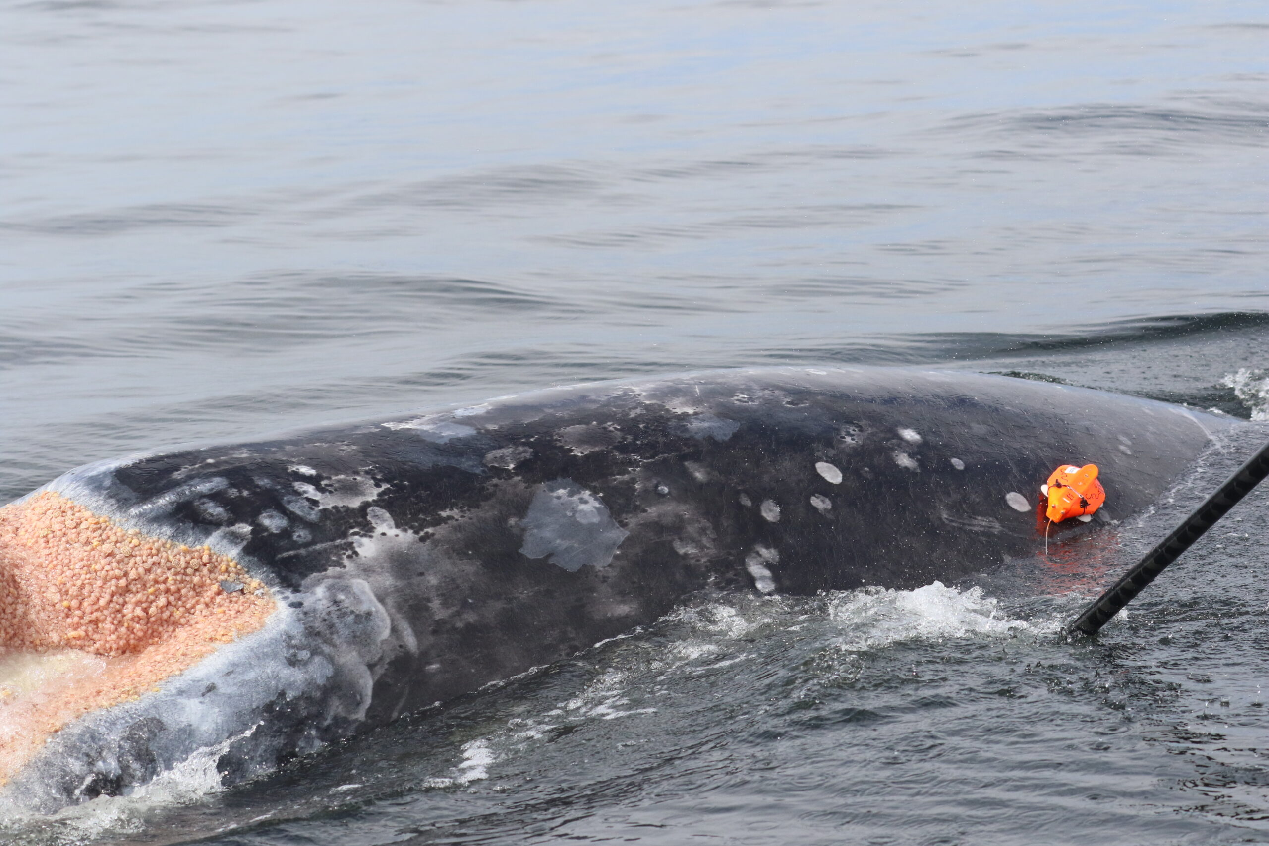
As you might remember from my earlier blog, the goal of my thesis is to use biologging data to define different foraging behaviors of Pacific Coast Feeding Group (PCFG) gray whales, and then calculate the energetic cost of those behaviors. I am defining PCFG foraging behaviors at two scales: (1) dives that represent different behavior states (e.g., travelling vs foraging), and (2) roll events, which are periods during dives where the whale is rolled onto their side, that represent different foraging tactics (e.g., headstanding vs side-swimming).
Initially, I was planning to use a clustering analysis to define these different foraging behaviors at both the dive and roll event scale, as this method has been used to successfully classify different foraging strategies for Galapagos sea lions (Schwarz et al., 2021). In short, this clustering analysis uses summary variables from events of interest to group events based on their similarity. These can be any metric that describes the event such as duration and depth, or body positioning variables like median pitch or roll. The output of the clustering analysis method results in groups of events that can each be used to define a different behavior.
However, while this method works for defining the foraging tactics of PCFG gray whales, my discussions with other scientists have suggested that there is a better method available for defining foraging behavior at the dive scale: Hidden Markov Models (HMMs). HMMs are similar to the clustering method described above in that they use summary variables at discrete time scales to define behavior states, but HMMs take into account the bias inherent to time series data – events that occur closer together in time are more likely to be more similar. This bias of time can confound clustering analyses, making HMMs a better tool for classifying a series of dives into different behavior states.
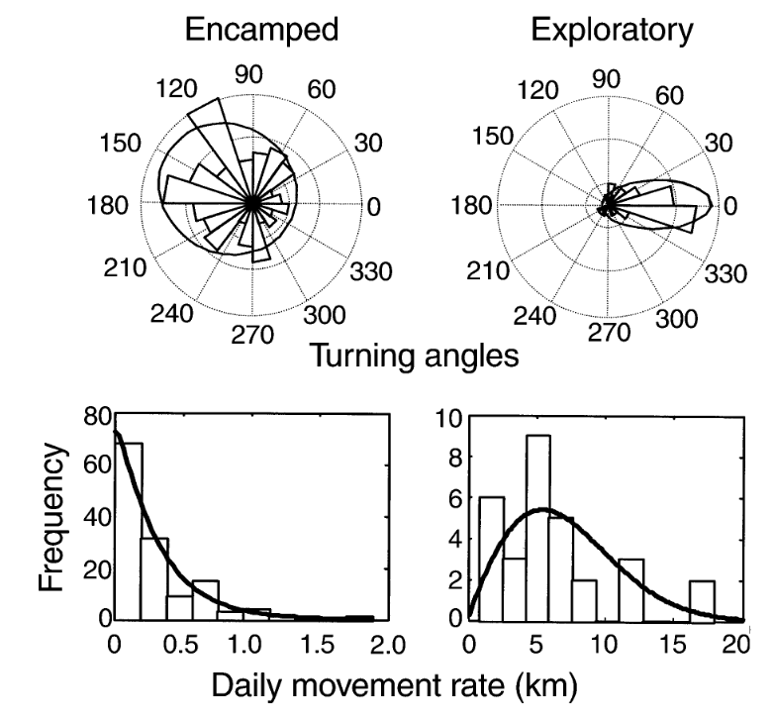
Like many analytical methods, the HMM framework was first proposed in a terrestrial system where it was used to classify the movement of translocated elk (Morales et al., 2004). The initial framework proposed using the step length, or the spatial distance between the animal’s locations at the start of subsequent time intervals, and the corresponding turning angle, to isolate “encamped” from “exploratory” behaviors in each elk’s movement path (Figure 1, from Morales et al., 2004). “Encamped” behaviors are those with short step lengths and high turning angles that show the individual is moving within a small area, and they can be associated with foraging behavior. On the other hand, “exploratory” behaviors are those with long step lengths and low turning angles that show the individual is moving in a relatively straight path and covering a lot of ground, which is likely associated with travelling behavior.
In the two decades following this initial framework proposed by Morales et al. (2004), the use of HMMs in anlaysis has been greatly expanded. One example of this expansion has been the development of mutlivariate HMMs that include additional data streams to supplement the step length and turning angle classification of “encamped” vs “exploratory” states in order to define more behaviors in movement data. For instance, a multivariate HMM was used to determine the impact of acoustic disturbance on blue whales (DeRuiter et al., 2017). In addition to step length and turning angle, dive duration and maximum depth, the duration of time spent at the surface following the dive, the number of feeding lunges in the dive, and the variability of the compass direction the whale was facing during the dive were all used to classify behavior states of the whales. This not only allowed for more behavior states to be identified (three instead of two as determined in the elk model), but also the differences in behavior states between individual animals included in the study, and the differences in the occurrence of behavior states due to changes in environmental noise.
The mutlivariate HMM used by DeRuiter et al. (2017) is a model I would ideally like to emulate with the biologging data from the PCFG gray whales. However, incorporating more variables invites more questions during the model construction process. For example, how many variables should be incorporated in the HMM? How should these variables be modeled? How many behavior states can be identified when including additional variables? These questions illustrate how easy it is to unnecessarily overcomplicate models and violate the principle of simiplicity toted by Albert Einstein, or to be overwhelmed by the complexity of these analytical tools.
Luckily, I can draw on the support of Gray whale Response to Ambient Noise Informed by Technology and Ecology (GRANITE) project collaborators Dr. Leslie New and Dr. Enrico Pirotta to guide my HMM model construction and assist in interpreting the outputs (Figure 2). With their help, I have been learning the importance of always asking if the change I am making to my model is biologically relevent to the PCFG gray whales, and if it will help give me more insight into the whales’ behavior. Even though using complex tools, such as Hidden Markov Models, has a steep learning curve, I know that this approach is not only placing this data analysis at the cutting edge of the field, but helping me practice fundamental skills, like model construction, that will pay off down the line in my career.
Sources
DeRuiter, S. L., Langrock, R., Skirbutas, T., Goldbogen, J. A., Calambokidis, J., Friedlaender, A. S., & Southall, B. L. (2017). A multivariate mixed Hidden Markov Model for blue whale behaviour and responses to sound exposure. Annals of Applied Statistics, 11(1), 362–392. https://doi.org/10.1214/16-AOAS1008
Morales, J. M., Haydon, D. T., Frair, J., Holsinger, K. E., & Fryxell, J. M. (2004). Extracting more out of relocation data: Building movement models as mixtures of random walks. Ecology, 85(9), 2436–2445. https://doi.org/10.1890/03-0269
Schwarz, J. F. L., Mews, S., DeRango, E. J., Langrock, R., Piedrahita, P., Páez-Rosas, D., & Krüger, O. (2021). Individuality counts: A new comprehensive approach to foraging strategies of a tropical marine predator. Oecologia, 195(2), 313–325. https://doi.org/10.1007/s00442-021-04850-w