Supporting marine life conservation as an outsider: Blue whales and earthquakes

By Mateo Estrada Jorge, Oregon State University undergraduate student, GEMM Lab REU Intern

Introduction

My name is Mateo Estrada and this past summer I had the pleasure of working with Dawn Barlow and Dr. Leigh Torres as a National Science Foundation (NSF) Research Experience for Undergraduates (REU) intern. I had the chance to proactively learn about the scientific method in the marine sciences by studying the acoustic behaviors of pygmy blue whales (Balaenoptera musculus brevicauda) that are documented residents of the South Taranaki Bight region in New Zealand (Torres 2013, Barlow et al. 2018). I’ve been interested in conducting scientific research since I began my undergraduate education at Oregon State University in 2015. Having the opportunity to apply the skills I gained through my education in this REU has been a blessing. I’m a physics and computer science major, but more than anything I’m a scientist and my passion has taken me in new, unexpected directions that I’m going to share in this blog post. My message for any students who feel like they haven’t found their path yet is: hang in there, sometimes it takes time for things to take shape. That has been my experience and I’m sure it’s been the experience of many people interested in the sciences. I’m a Physics and Computer Science student, so why am I studying blue whales, and more specifically, how can I be doing marine science research having only taken intro to biology 101?

My background

I decided to apply for the REU in the Spring 2021 because it was a chance to use my programming skills in the marine sciences. I’m also passionate about conservation and protecting the environment in a pragmatic way, so I decided to find a niche where I could put my technical skills to good use. Finally, I wanted to explore a scientific field outside of my area of expertise to grow as a student and to learn from other researchers. I was mostly inspired by anecdotal tales of Physicist Richard Feynman who would venture out of the physics department at Caltech and into other departments to learn about what other scientists were investigating to inspire his own work. This summer, I ventured into the world of marine science, and what I found in my project was fascinating.

Whale watching tour

Figure 1. Me standing on a boat on the Pacific Ocean off Long Beach, CA.

To get into the research mode, I decided to go on a whale watching tour with the Aquarium of the Pacific. The tour was two hours long and the sunburn was worth it because we got to see four blue whales off the Long Beach coast in California. I got to see the famous blue whale blow and their splashes. It was the first time I was on a big boat in the ocean, so naturally I got seasick (Fig 1). But it was exciting to get a chance to see blue whales in action (luckily, I didn’t actually hurl). The marine biologist onboard also gave a quick lecture on the relative size of blue whales and some of their behaviors. She also pointed out that they don’t use Sonar to locate whales as this has been shown to disturb their calling behaviors. Instead, we looked for a blow and splashing. The tour was a wonderful experience and I’m glad I got to see some whales out in nature. This experience also served as a reminder of the beauty of marine life and the responsibility I feel for trying to understand and help conserving it.

Context of blue whale calling

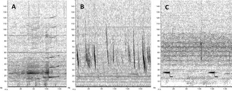
Sound plays a significant role in the marine environment and is a critical mode of communication for many marine animals including baleen whales. Blue whales produce different vocalizations, otherwise known as calls.  Blue whale song is theorized to be produced by males of the species as a form of reproductive behavior, similar to how male peacocks engage females by displaying their elongated upper tail covert feathers in iridescent colors as a courtship mechanism. Then there are “D calls” that are associated with social mechanisms while foraging, and these calls are made by both female and male blue whales (Lewis et al. 2018) (Fig. 2).

Figure 2. Spectrogram of Pygmy blue whale D calls manually (and automatically) selected, frequency 0-150 Hz.

Understanding research on blue whales

The most difficult part about coming into a project as an outsider is catching up. I learned how anthropogenetic (human made) noise affects blue whale communication. For example, it has been showing that Mid Frequency Active Sonar signals employed by the U.S. Navy affect blue whale D calling patterns (Melcón 2012). Furthermore, noise from seismic airguns used for oil and gas exploration has also impact blue whale calling behavior (Di Lorio, 2010). Understanding the environmental context in which the pygmy blue whales live and the anthropogenic pressures they face is essential in marine conservation. Protecting the areas in which they live is important so they can feed, reproduce and thrive effectively. What began as a slowly falling snowflake at the start of a snowstorm turned into a cascading avalanche of knowledge pouring into my mind in just two weeks.
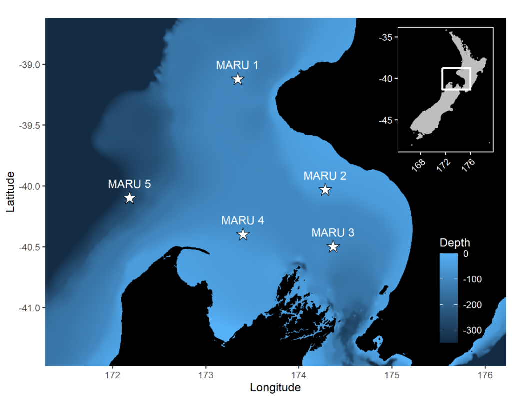
Figure 3. The white stars show the hydrophone locations (n = 5). A bathymetric scale of the depth is also given.

The research question I set out to tackle in my internship was: do blue whales change their calling behavior in response to natural noise events from earthquake activity? To do this, I used acoustic recordings from five hydrophones deployed in the South Taranaki Bight (Fig. 3), paired with an existing dataset of all recorded earthquakes in New Zealand (GeoNet). I identified known earthquakes in our acoustic recordings, and then examined the blue whale D calls during 4 hours before and after each earthquake event to look for any change in the number of calls, call energy, entropy, or bandwidth.

A great mentor and lab team

The days kept passing and blending into each other, as they often do with remote work. I began to feel isolated from the people I was working with and the blue whales I was studying. The zoom calls, group chats, and working alongside other remote interns kept me afloat as I adapted to a work world fully online. Nevertheless, I was happy to continue working on this project because I felt like I was slowly becoming part of the GEMM Lab. I would meet with my mentor Dawn Barlow at least once a week and we would spend time talking about the project and sorting out the difficult details of data processing. She always encouraged my curiosity to ask questions. Even if they were silly questions, she was happy to ponder them because she is a curious scientist like myself.

What we learned

Pygmy blue whales from the South Taranaki Bight region do not change their acoustic behavior in response to earthquake activity. The energy of the earthquake, magnitude, depth, and distance to the origin all had no influence on the number of blue whale D calls, the energy of their calling, the entropy, and the bandwidth. A likely reason for why the blue whales would have no acoustic response to earthquakes (magnitude < 5) is that the STB region is a seismically active region due to the nearby interface of the Australian and Pacific plates. Because of the plate tectonics, the region averages about 20,000 recorded earthquakes per year (GeoNet: Earthquake Statistics). Given that pygmy blue whales are present in the STB region year-round (Barlow et al. 2018), the blue whales may have adapted to tolerate the earthquake activity (Fig 4).
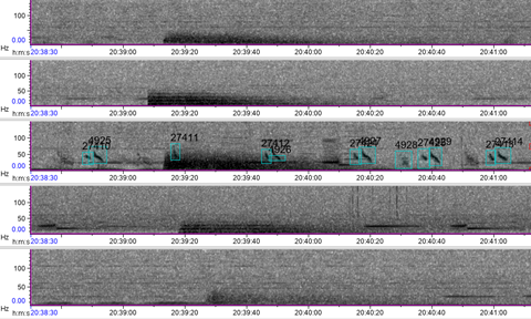
Figure 4. Earthquake signal from MARU (1, 2, 3, 4, 5) and blue whale D calls, Frequency 0-150 Hz.

Looking at the future

I presented my work at the end of my REU internship program, which was a difficult challenge for me because I am often intimidated by public speaking (who isn’t?). Communicating science has always been a big interest of me. I love reading news articles about new breakthroughs and being a small part of that is a huge privilege for me. Finding my own voice and having new insights to contribute to the scientific world has always been my main objective. Now I will get to deliver a poster presentation of my REU work at the Association for the Sciences of Limnology and Oceanography (ASLO) Conference in March 2022. I am both excited and nervous to take on this new adventure of meeting seasoned professionals, communicating my results, and learning about the ocean sciences. I hope to gain new inspirations for my future academic and professional work.

References:

About Earthquake Drums – GeoNet. geonet.Org. Retrieved June 23, 2021, from https://www.geonet.org.nz/about/earthquake/drums

Barlow, D. R., Torres, L. G., Hodge, K. B., Steel, D., Scott Baker, C., Chandler, T. E., Bott, N., Constantine, R., Double, M. C., Gill, P., Glasgow, D., Hamner, R. M., Lilley, C., Ogle, M., Olson, P. A., Peters, C., Stockin, K. A., Tessaglia-Hymes, C. T., & Klinck, H. (2018). Documentation of a New Zealand blue whale population based on multiple lines of evidence. Endangered Species Research, 36, 27–40. https://doi.org/10.3354/esr00891

Di Iorio, L., & Clark, C. W. (2010). Exposure to seismic survey alters blue whale acoustic communication. Biology Letters, 6(3), 334–335. https://doi.org/10.1098/rsbl.2009.0967

Lewis, L. A., Calambokidis, J., Stimpert, A. K., Fahlbusch, J., Friedlaender, A. S., McKenna, M. F., Mesnick, S. L., Oleson, E. M., Southall, B. L., Szesciorka, A. R., & Sirović, A. (2018). Context-dependent variability in blue whale acoustic behaviour. Royal Society Open Science, 5(8). https://doi.org/10.1098/rsos.180241

Melcón, M. L., Cummins, A. J., Kerosky, S. M., Roche, L. K., Wiggins, S. M., & Hildebrand, J. A. (2012). Blue whales respond to anthropogenic noise. PLoS ONE, 7(2), 1–6. https://doi.org/10.1371/journal.pone.0032681

Torres LG. 2013 Evidence for an unrecognised blue whale foraging ground in New Zealand. NZ J. Mar. Freshwater Res. 47, 235–248. (doi:10. 1080/00288330.2013.773919)

Inference, and the intersection of ecology and statistics

By Dawn Barlow, PhD student, OSU Department of Fisheries and Wildlife, Geospatial Ecology of Marine Megafauna Lab

Recently, I had the opportunity to attend the International Statistical Ecology Conference (ISEC), a biennial meeting of researchers at the interface of ecology and statistics. I am a marine ecologist, fascinated by the interactions between animals and the dynamic ocean environment they inhabit. If you had asked me five years ago whether I thought I would ever consider myself a statistician or a computer programmer, my answer would certainly have been “no”. Now, I find myself studying the ecology of blue whales in New Zealand using a variety of data streams and methodologies, but a central theme for my dissertation is species distribution modeling. Species distribution models (SDMs) are mathematical algorithms that correlate observations of a species with environmental conditions at their observed locations to gain ecological insight and predict spatial distributions of the species (Fig. 1; Elith and Leathwick 2009). I still can’t say I would identify as a statistician, but I have a growing appreciation for the role of statistics to gain inference in ecology.

Figure 1. A schematic of a species distribution model (SDM) illustrating how the relationship between mapped species and environmental data (left) is compared to describe “environmental space” (center), and then map predictions from a model using only environmental predictors (right). Note that inter-site distances in geographic space might be quite different from those in environmental space—a and c are close geographically, but not environmentally. The patterning in the predictions reflects the spatial autocorrelation of the environmental predictors. Figure reproduced from Elith and Leathwick (2009).

Before I continue, let’s take a look at just a few definitions from Merriam-Webster’s dictionary:

Statistics: a branch of mathematics dealing with the collection, analysis, interpretation, and presentation of masses of numerical data

Ecology: a branch of science concerned with the interrelationship of organisms and their environments

Inference: a conclusion or opinion that is formed because of known facts or evidence

Ecological data are notoriously noisy, messy, and complex. Statistical tests are meant to help us understand whether a pattern in the data is different from what we would expect through random chance. When we study how organisms interact with one another and their environment, it is impossible to completely capture all elements of the ecosystem. Therefore, ecology is a field ripe with challenges for statisticians. How do we quantify a meaningful biological signal amidst all the noise? How can we gain inference from ecological data to enhance knowledge, and how can we use that knowledge to make informed predictions? Marine mammals are notoriously difficult to study. They inhabit an environment that is relatively inaccessible and inhospitable to humans, they occur in low numbers, they are highly mobile, and they are rarely visible. All ecological data are difficult and noisy and riddled with small sample sizes, but counting trees presents fewer logistical challenges than counting moving whales in an ever-changing open-ocean setting. Therefore, new methodologies in areas like species distribution modeling are often developed using large, terrestrial datasets and eventually migrate to applications in the marine environment (Robinson et al. 2011).

Many presentations I attended at the conference were geared toward moving beyond correlative SDMs. SDMs were developed to correlate species occurrence patterns with features of the environment they inhabit (e.g. temperature, precipitation, terrain, etc.). However, those relationships do not actually explain the underlying mechanism of why a species is more likely to occur in one environment compared to another. Therefore, ecological statisticians are now using additional information and modeling approaches within SDMs to incorporate information such as species co-occurrence patterns, population demographic information, and physiological constraints. Building SDMs to include such process-explicit information allows us to make steps toward understanding not just when and where a species occurs, but why.

Machine learning is an area that continues to advance and open doors to new applications in ecology. Machine learning approaches differ fundamentally from classical statistics. In statistics, we formulate a hypothesis, select the appropriate model to test that hypothesis (for example, linear regression), then test how well the data fit the model (“Is the relationship linear?”), and test the strength of that inference (“Is the linear pattern different from what we would expect due to random chance?”). Machine learning, on the other hand, does not use a predetermined notion of relationships between variables. Rather, it tries to create an algorithm that fits the patterns in the data. Statistics asks how well the data fit a model, and machine learning asks how well a model fits the data.

Machine learning approaches allow for very complex relationships to be included in models and can be excellent for making predictions. However, sometimes the relationships fitted by a machine learning algorithm are so complex that it is not possible to infer any ecological meaning from them. As one ISEC presenter put it, in machine learning “the computer learns but the scientist does not”. The most important thing when selecting your methodology is to remember your question and your goal. Do you want to understand the mechanism of why an animal is where it is? Or do you not need to understand the driver, but rather want to make the best predictions of where an animal will be? In my case, the answer to that question differs from one of my PhD chapters to the next. We want to understand the functional relationships between oceanography, krill availability, and blue whale distribution (Barlow et al. 2020), and subsequently we want to develop forecasting models that can reliably predict blue whale distribution to inform conservation efforts (Fig. 2).

Figure 2. An example predictive map of where we expect blue whales to be distributed based on environmental conditions. Warmer colors represent areas with a higher probability of blue whale occurrence, and the blue crosses represent locations where blue whales were observed.

ISEC was an excellent opportunity for me to break out of my usual marine mammal-centered bubble and get a taste of what is happening on the leading edge of statistical ecology. I learned about the latest approaches and innovations in species distribution modeling, and in the process I also learned about trees, koalas, birds, and many other organisms from around the world. A fun bonus of attending a methods-focused conference is learning about completely new study species and systems. There are many ways of approaching an ecological question, gaining inference, and making predictions. I look forward to incorporating the knowledge I gained through ISEC into my own research, both in my doctoral work and in applications of new methods to future research projects.

Figure 3. The virtual conference photo of all who attended the biennial International Statistical Ecology Conference. Thank you to the organizers, who made it a truly excellent and engaging conference experience!

References

Barlow, D.R., Bernard, K.S., Escobar-Flores, P., Palacios, D.M., and Torres, L.G. 2020. Links in the trophic chain: Modeling functional relationships between in situ oceanography, krill, and blue whale distribution under different oceanographic regimes. Mar. Ecol. Prog. Ser. doi:https://doi.org/10.3354/meps13339.

Elith, J., and Leathwick, J.R. 2009. Species Distribution Models: Ecological Explanation and Prediction Across Space and Time. Annu. Rev. Ecol. Evol. Syst. 40(1): 677–697. doi:10.1146/annurev.ecolsys.110308.120159.

Robinson, L.M., Elith, J., Hobday, A.J., Pearson, R.G., Kendall, B.E., Possingham, H.P., and Richardson, A.J. 2011. Pushing the limits in marine species distribution modelling: Lessons from the land present challenges and opportunities. doi:10.1111/j.1466-8238.2010.00636.x.

It all starts with the wind: The importance of upwelling

By Dawn Barlow, PhD student, OSU Department of Fisheries and Wildlife, Geospatial Ecology of Marine Megafauna Lab

The focus of my PhD research is on the ecology and distribution of blue whales in New Zealand. However, it has been a long time since I’ve seen a blue whale, and much of my time recently has been spent thinking about wind. What does wind matter to a blue whale? It actually matters a whole lot, because the wind drives an important biological process in many coastal oceans called upwelling. Wind blowing along shore, paired with the rotation of the earth, leads to a net movement of surface waters offshore (Fig. 1). As the surface water is pushed away, it is replaced by cold, nutrient-rich water from much deeper. When those nutrients become exposed to sunlight, they provide sustenance for the little planktonic lifeforms in the ocean, which in turn provide food for much larger predators including marine mammals such as blue whales. This “wind-to-whales” trophic pathway was coined by Croll et al. (2005), who demonstrated that off the West Coast of the United States, aggregations of whales could be expected downstream of upwelling centers, in concert with high productivity and abundant krill prey.

Figure 1. Graphic of the upwelling process, illustrating that when the wind blows along shore, surface waters are replaced by deeper water that is cold and nutrient rich. Source: NOAA
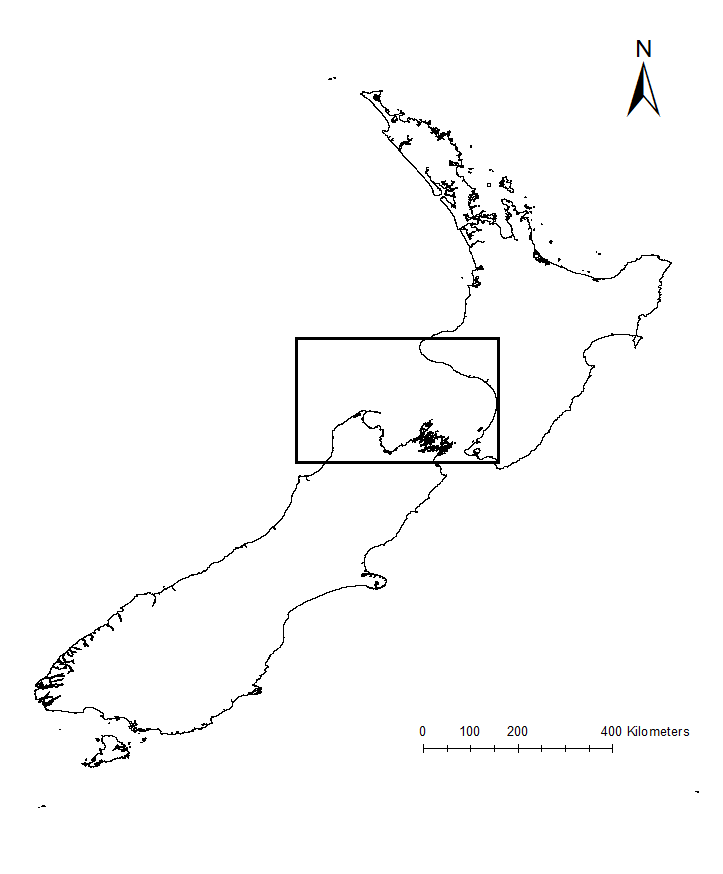
Figure 2. Map of New Zealand, with the South Taranaki Bight region (STB) denoted by the black box.

Much of what is understood today about upwelling comes from decades of research on the California Current ecosystem off the West Coast of the United States. Yet, the focus of my research is on an upwelling system on the other side of the world, in the South Taranaki Bight region (STB) of New Zealand (Fig. 2). In the case of the STB, westerly winds over Kahurangi Shoals lead to decreased sea level nearshore, forcing cold, nutrient rich waters to rise to the surface. The wind, along with the persistence of the Westland Current, then pushes a cold and productive plume of upwelled waters around Cape Farewell and into the STB (Fig. 3; Shirtcliffe et al. 1990).

Figure 3. Satellite image of the cold water plume in the South Taranaki Bight, indicative of upwelling. The origin of the upwelling at Kahurangi Shoals, Cape Farewell, and the typical path of the upwelling plume are denoted.

Through research conducted by the GEMM Lab over the years, we have demonstrated that blue whales utilize the STB region for foraging (Torres 2013, Barlow et al. 2018). Recent research on the oceanography of the STB region has further illuminated the mechanisms of this upwelling system, including the path and persistence of the upwelling plume in the STB across years and seasons (Chiswell et al. 2017, Stevens et al. 2019). However, the wind-to-whales pathway has not yet been described for this part of the world, and that is where the next section of my PhD research comes in. The whole system does not respond instantaneously to wind; the pathway from wind to whales takes time. But how much time is required for each step? How long after a strong wind event can we expect aggregations of feeding blue whales? These are some of the questions I am trying to tackle. For example, we hypothesize that some of the mechanisms and their respective lag times can be sketched out as follows:

Figure 4. The wind-to-whales trophic pathway, and hypothesized lags between steps.

All of these questions involve integrating oceanography, satellite imagery, wind data, and lag times, leading me to delve into many different analytical approaches including time series analysis and predictive modeling. If we are able to understand the lag times along this series of events leading to blue whale feeding opportunities, then we may be able to forecast blue whale occurrence in the STB based on the current wind and upwelling conditions. Forecasting with some amount of lead time could be a very powerful management tool, allowing for protection measures that are dynamic in space and time and therefore more effective in conserving this blue whale population and balancing human impacts.

Figure 5. A blue whale lunges on a patch of krill. The end of the wind-to-whales pathway. Drone piloted by Todd Chandler.

References:

Barlow DR, Torres LG, Hodge KB, Steel D, Baker CS, Chandler TE, Bott N, Constantine R, Double MC, Gill P, Glasgow D, Hamner RM, Lilley C, Ogle M, Olson PA, Peters C, Stockin KA, Tessaglia-hymes CT, Klinck H (2018) Documentation of a New Zealand blue whale population based on multiple lines of evidence. Endanger Species Res 36:27–40.

Chiswell SM, Zeldis JR, Hadfield MG, Pinkerton MH (2017) Wind-driven upwelling and surface chlorophyll blooms in Greater Cook Strait. New Zeal J Mar Freshw Res.

Croll DA, Marinovic B, Benson S, Chavez FP, Black N, Ternullo R, Tershy BR (2005) From wind to whales: Trophic links in a coastal upwelling system. Mar Ecol Prog Ser 289:117–130.

Shirtcliffe TGL, Moore MI, Cole AG, Viner AB, Baldwin R, Chapman B (1990) Dynamics of the Cape Farewell upwelling plume, New Zealand. New Zeal J Mar Freshw Res 24:555–568.

Stevens CL, O’Callaghan JM, Chiswell SM, Hadfield MG (2019) Physical oceanography of New Zealand/Aotearoa shelf seas–a review. New Zeal J Mar Freshw Res.

Torres LG (2013) Evidence for an unrecognised blue whale foraging ground in New Zealand. New Zeal J Mar Freshw Res 47:235–248.

Classifying cetacean behavior

Clara Bird, Masters Student, OSU Department of Fisheries and Wildlife, Geospatial Ecology of Marine Megafauna Lab

The GEMM lab recently completed its fourth field season studying gray whales along the Oregon coast. The 2019 field season was an especially exciting one, we collected rare footage of several interesting gray whale behaviors including GoPro footage of a gray whale feeding on the seafloor, drone footage of a gray whale breaching, and drone footage of surface feeding (check out our recently released highlight video here). For my master’s thesis, I’ll use the drone footage to analyze gray whale behavior and how it varies across space, time, and individual. But before I ask how behavior is related to other variables, I need to understand how to best classify the behaviors.

How do we collect data on behavior?

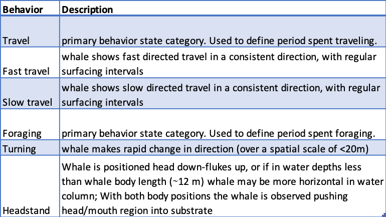
One of the most important tools in behavioral ecology is an ‘ethogram’. An ethogram is a list of defined behaviors that the researcher expects to see based on prior knowledge. It is important because it provides a standardized list of behaviors so the data can be properly analyzed. For example, without an ethogram, someone observing human behavior could say that their subject was walking on one occasion, but then say strolling on a different occasion when they actually meant walking. It is important to pre-determine how behaviors will be recorded so that data classification is consistent throughout the study. Table 1 provides a sample from the ethogram I use to analyze gray whale behavior. The specificity of the behaviors depends on how the data is collected.

Table 1. Sample from gray whale ethogram. Based on ethogram from Torres et al. (2018).

In marine mammal ecology, it is challenging to define specific behaviors because from the traditional viewpoint of a boat, we can only see what the individuals are doing at the surface. The most common method of collecting behavioral data is called a ‘focal follow’. In focal follows an individual, or group, is followed for a set period of time and its behavioral state is recorded at set intervals.  For example, a researcher might decide to follow an animal for an hour and record its behavioral state at each minute (Mann 1999). In some studies, they also recorded the location of the whale at each time point. When we use drones our methods are a little different; we collect behavioral data in the form of continuous 15-minute videos of the whale. While we collect data for a shorter amount of time than a typical focal follow, we can analyze the whole video and record what the whale was doing at each second with the added benefit of being able to review the video to ensure accuracy. Additionally, from the drone’s perspective, we can see what the whales are doing below the surface, which can dramatically improve our ability to identify and describe behaviors (Torres et al. 2018).

Categorizing Behaviors

In our ethogram, the behaviors are already categorized into primary states. Primary states are the broadest behavioral states, and in my study, they are foraging, traveling, socializing, and resting. We categorize the specific behaviors we observe in the drone videos into these categories because they are associated with the function of a behavior. While our categorization is based on prior knowledge and critical evaluation, this process can still be somewhat subjective.  Quantitative methods provide an objective interpretation of the behaviors that can confirm our broad categorization and provide insight into relationships between categories.  These methods include path characterization, cluster analysis, and sequence analysis.

Path characterization classifies behaviors using characteristics of their track line, this method is similar to the RST method that fellow GEMM lab graduate student Lisa Hildebrand described in a recent blog. Mayo and Marx (1990) analyzed the paths of surface foraging North Atlantic Right Whales and were able to classify the paths into primary states; they found that the path of a traveling whale was more linear and then paths of foraging or socializing whales that were more convoluted (Fig 1). I plan to analyze the drone GPS track line as a proxy for the whale’s track line to help distinguish between traveling and foraging in the cases where the 15-minute snapshot does not provide enough context.

Figure 1. Figure from Mayo and Marx (1990) showing different track lines symbolized by behavior category.

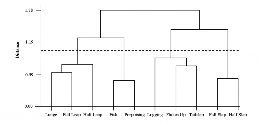
Cluster analysis looks for natural groupings in behavior. For example, Hastie et al. (2004) used cluster analysis to find that there were four natural groupings of bottlenose dolphin surface behaviors (Fig. 2). I am considering using this method to see if there are natural groupings of behaviors within the foraging primary state that might relate to different prey types or habitat. This process is analogous to breaking human foraging down into sub-categories like fishing or farming by looking for different foraging behaviors that typically occur together.

Figure 2. Figure from Hastie et al. (2004) showing the results of a hierarchical cluster analysis.

Lastly, sequence analysis also looks for groupings of behaviors but, unlike cluster analysis, it also uses the order in which behaviors occur. Slooten (1994) used this method to classify Hector’s dolphin surface behaviors and found that there were five classes of behaviors and certain behaviors connected the different categories (Fig. 3). This method is interesting because if there are certain behaviors that are consistently in the same order then that indicates that the order of events is important. What function does a specific sequence of behaviors provide that the behaviors out of that order do not?

Figure 3. Figure from Slooten (1994) showing the results of sequence analysis.

Think about harvesting fruits and vegetables from a garden: the order of how things are done matters and you might use different methods to harvest different kinds of produce. Without knowing what food was being harvested, these methods could detect that there were different harvesting methods for different fruits or veggies. By then studying when and where the different methods were used and by whom, we could gain insight into the different functions and patterns associated with the different behaviors. We might be able to detect that some methods were always used in certain habitat types or that different methods were consistently used at different times of the year.

Behavior classification methods such as these described provide a more refined and detailed analysis of categories that can then be used to identify patterns of gray whale behaviors. While our ultimate goal is to understand how gray whales will be affected by a changing environment, a comprehensive understanding of their current behavior serves as a baseline for that future study.

References

Burnett, J. D., Lemos, L., Barlow, D., Wing, M. G., Chandler, T., & Torres, L. G. (2019). Estimating morphometric attributes of baleen whales with photogrammetry from small UASs: A case study with blue and gray whales. Marine Mammal Science, 35(1), 108–139. https://doi.org/10.1111/mms.12527

Darling, J. D., Keogh, K. E., & Steeves, T. E. (1998). Gray whale (Eschrichtius robustus) habitat utilization and prey species off Vancouver Island, B.C. Marine Mammal Science, 14(4), 692–720. https://doi.org/10.1111/j.1748-7692.1998.tb00757.x

Hastie, G. D., Wilson, B., Wilson, L. J., Parsons, K. M., & Thompson, P. M. (2004). Functional mechanisms underlying cetacean distribution patterns: Hotspots for bottlenose dolphins are linked to foraging. Marine Biology, 144(2), 397–403. https://doi.org/10.1007/s00227-003-1195-4

Mann, J. (1999). Behavioral sampling methods for cetaceans: A review and critique. Marine Mammal Science, 15(1), 102–122. https://doi.org/10.1111/j.1748-7692.1999.tb00784.x

Slooten, E. (1994). Behavior of Hector’s Dolphin: Classifying Behavior by Sequence Analysis. Journal of Mammalogy, 75(4), 956–964. https://doi.org/10.2307/1382477

Torres, L. G., Nieukirk, S. L., Lemos, L., & Chandler, T. E. (2018). Drone up! Quantifying whale behavior from a new perspective improves observational capacity. Frontiers in Marine Science, 5(SEP). https://doi.org/10.3389/fmars.2018.00319

Mayo, C. A., & Marx, M. K. (1990). Surface foraging behaviour of the North Atlantic right whale, Eubalaena glacialis, and associated zooplankton characteristics. Canadian Journal of Zoology, 68(10), 2214–2220. https://doi.org/10.1139/z90-308

Detecting blue whales from acoustic data

By Dawn Barlow, PhD student, OSU Department of Fisheries and Wildlife, Geospatial Ecology of Marine Megafauna Lab

In January of 2016, five underwater recording units were dropped to the seafloor in New Zealand to listen for blue whales (Fig. 1). These hydrophones sat listening for two years, brought to the surface only briefly every six months to swap out batteries and offload the data. Through all seasons and conditions when scientists couldn’t be on the water, they recorded the soundscape, generating a wealth of acoustic data with the potential to greatly expand our knowledge of blue whale ecology

Figure 1. Locations of the five Marine Autonomous Recording Units (MARUs) in the South Taranaki Bight region of New Zealand.

We have established that blue whales are present in New Zealand waters year-round 1. However, many questions remain regarding their distribution across daily, seasonal, and yearly scales. Our two-year acoustic dataset from five hydrophones throughout the STB region is a goldmine of information on blue whale occurrence patterns and the soundscape they inhabit. Having year-round occurrence data will allow us to examine what environmental and anthropogenic factors may influence blue whale distribution patterns. The hydrophones were listening for whales around the clock, every day, while we were on the other side of the world awaiting the recovery of the data to answer our questions.

Before any questions of seasonal distribution or anthropogenic impacts and noise can be addressed, however, we need to know something far more basic: when and where did we record blue whale vocalizations? This may seem like a simple, stepping-stone question, but it is actually quite involved, and the reason I spent the last month working with a team of acousticians at Cornell University’s Center for Conservation Bioacoustics. The expert research group here at Cornell, led by Dr. Holger Klinck, have been instrumental in our New Zealand blue whale research, including developing and building the recording units, hydrophone deployment and recovery, data processing, analysis, and advice. I am thrilled to work with all of them, and had an incredibly productive month of learning about acoustics from the best.

Blue whales produce multiple vocalizations that we are interested in documenting. The New Zealand song (Fig. 2A) is highly stereotyped and unique to the Southwest Pacific Ocean 2,3. Low-frequency downsweeps, or “D calls” (Fig. 2B), are far more variable and produced by blue whale populations around the world 4. Furthermore, Antarctic blue whales produce a highly-stereotyped “Z call” (Fig. 2C) and are known to be present in New Zealand waters occasionally 5.

Figure 2. Spectrograms of (A) the New Zealand blue whale song, (B), D calls, and (C) Antarctic Z calls.

One way to determine when blue whales were vocalizing is for an analyst to manually review the entirety of the two years of sound recordings for each of the five hydrophones by hand to scan for and select individual vocalizations. An alternative approach is to develop a detector algorithm to locate calls in the data based on their stereotypical characteristics. Over the past month I built, tested, and ran detectors for each blue whale call type using what is called a data template detector. This technique uses example signals from the data that the analyst selects as templates. The templates should be clear signals, and representative of the variation in calls contained in the dataset. Then, by comparing pixel characteristics between the template spectrograms and the spectrogram of the recording of interest using certain matching criteria (e.g. threshold for spectrogram correlation, detection frequency range), the algorithm searches for other signals like the templates in the full dataset. For example, in Fig. 3 you can see units of blue whale song I selected as templates for my detector.

Figure 3. Spectrogram of selected sound clips of New Zealand blue whale song, with units used as templates for a detector shown inside the teal boxes.

Testing the performance of a detector algorithm is critical. Therefore, a dataset is needed where calls were identified by an analyst and then used as the “ground truth”, to which the detector results are compared. For my ground truth dataset, I took a subset of 52 days and hand-browsed the spectrograms to identify and log New Zealand blue whale song, D calls, and Antarctic Z calls. In evaluating detector performance, there are three important metrics that need to be weighed: precision (the proportion of detections that are true), recall (the proportion of true calls identified by the detector), and false alarm rate (the number of false positive detections per hour). Ideally, the detector should be optimized to maximize precision and recall and minimize the false positives.

The STB region is highly industrial, and our two-year acoustic dataset contains periods of pervasive seismic airgun noise from oil and gas exploration. Ideally, a detector would be able to identify blue whale vocalizations even in the presence of airgun operations that dominate the soundscape for months. For blue whale song, the detector did quite well! With a precision of 0.91 and recall of 0.93, the detector could pick out song units over airgun noise (Fig. 4). A false alarm rate of 8 false positives per hour is a sacrifice worth making to identify song during seismic operations (and the false positives will be removed in a subsequent step). For D calls, seismic survey activity presented a different challenge. While the detector did well at identifying D calls during airgun operation, the first several detector attempts also logged every single airgun blast as a blue whale vocalization—clearly problematic. Through an iterative process of selecting template signals, and adjusting the number of templates used and the correlation threshold, I was able to come up with a detector which selected D calls and missed most airgun blasts. This success felt like a victory.

Figure 4. An example of spectrograms of simultaneous recordings from the five hydrophones illustrating seismic airgun noise (strong broadband signals that appear as repetitive black, vertical lines) overlapping New Zealand blue whale song. The red boxes are detection events selected by the detector, demonstrating its ability to capture song even during airgun operation.

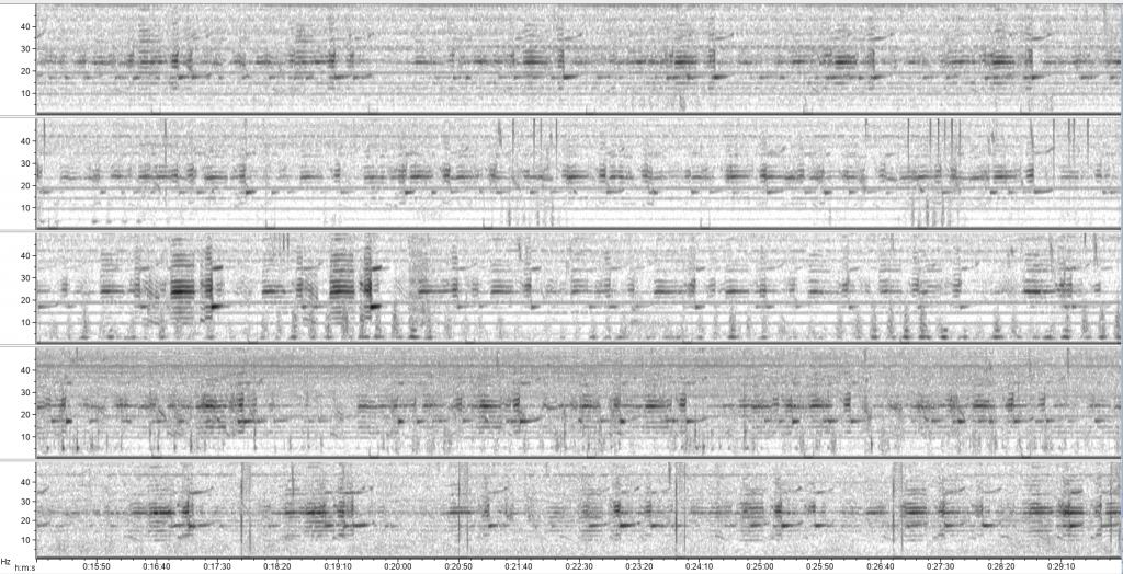
After this detector development and validation process, I ran each detector on the full two-year acoustic dataset for all five recording units. This step was a good exercise in patience as I eagerly awaited the outputs for the many hours they took to run. The next step in the process will be for me to go through and validate each detector event to eliminate any false positives. However, running the detectors on the full dataset has allowed for exciting preliminary examinations of seasonal blue whale acoustic patterns, which need to be refined and expanded upon as the analysis continues. For example, sometimes the New Zealand song dominates the recordings on all hydrophones (Fig. 5), whereas other times of year song is less common. Similarly, there appear to be seasonal patterns in D calls and Antarctic Z calls, with peaks and dips in detections during different times of year.

Figure 5. An example spectrogram of simultaneous recordings from all five hydrophones during a time when New Zealand blue whale song dominated the recordings, with numerous, overlapping calls.

As with many things, the more questions you ask, the more questions you come up with. From preliminary explorations of the acoustic data my head is buzzing with ideas for further analysis and with new questions I hadn’t thought to ask of the data before. My curiosity has been fueled by scrolling through spectrograms, looking, and listening, and I am as excited as ever to continue researching blue whale ecology. I would like to thank the team at the Center for Conservation Bioacoustics for their support and guidance over the past month, and I look forward to digging deeper into the stories being told in the acoustic data!

Figure 6. A pair of blue whales observed in February 2017 in the South Taranaki Bight. Photo: L. Torres.

References

1.          Barlow, D. R. et al. Documentation of a New Zealand blue whale population based on multiple lines of evidence. Endanger. Species Res. 36, 27–40 (2018).

2.          McDonald, M. A., Mesnick, S. L. & Hildebrand, J. A. Biogeographic characterisation of blue whale song worldwide: using song to identify populations. J. Cetacean Res. Manag. 8, 55–65 (2006).

3.          Balcazar, N. E. et al. Calls reveal population structure of blue whales across the Southeast Indian Ocean and the Southwest Pacific Ocean. J. Mammal. 96, 1184–1193 (2015).

4.          Oleson, E. M. et al. Behavioral context of call production by eastern North Pacific blue whales. Mar. Ecol. Prog. Ser. 330, 269–284 (2007).

5.          McDonald, M. A. An acoustic survey of baleen whales off Great Barrier Island, New Zealand. New Zeal. J. Mar. Freshw. Res. 40, 519–529 (2006).


Eyes from Space: Using Remote Sensing as a Tool to Study the Ecology of Blue Whales

By Christina Garvey, University of Maryland, GEMM Lab REU Intern

It is July 8th and it is my 4th week here in Hatfield as an REU intern for Dr. Leigh Torres. My name is Christina Garvey and this summer I am studying the spatial ecology of blue whales in the South Taranaki Bight, New Zealand. Coming from the east coast, Oregon has given me an experience of a lifetime – the rugged shorelines continue to take my breath away and watching sea lions in Yaquina Bay never gets old. However, working on my first research project has by far been the greatest opportunity and I have learned so much in so little time. When Dr. Torres asked me to contribute to this blog I was unsure of how I would write about my work thus far but I am excited to have the opportunity to share the knowledge I have gained with whoever reads this blog post.

The research project that I will be conducting this summer will use remotely sensed environmental data (information collected from satellites) to predict blue whale distribution in the South Taranaki Bight (STB), New Zealand. Those that have read previous blogs about this research may remember that the STB study area is created by a large indentation or “bight” on the southern end of the Northern Island. Based on multiple lines of evidence, Dr. Leigh Torres hypothesized the presence of an unrecognized blue whale foraging ground in the STB (Torres 2013). Dr. Torres and her team have since proved that blue whales frequent this region year-round; however, the STB is also very industrial making this space-use overlap a conservation concern (Barlow et al. 2018). The increasing presence of marine industrial activity in the STB is expected to put more pressure on blue whales in this region, whom are already vulnerable from the effects of past commercial whaling (Barlow et al. 2018) If you want to read more about blue whales in the STB check out previous blog posts that talk all about it!

Figure 1. A blue whale surfaces in front of a floating production storage and offloading vessel servicing the oil rigs in the South Taranaki Bight. Photo by D. Barlow.

Figure 2. South Taranaki Bight, New Zealand, our study site outlined by the red box. Kahurangi Point (black star) is the site of wind-driven upwelling system.

The possibility of the STB as an important foraging ground for a resident population of blue whales poses management concerns as New Zealand will have to balance industrial growth with the protection and conservation of a critically endangered species. As a result of strong public support, there are political plans to implement a marine protected area (MPA) in the STB for the blue whales. The purpose of our research is to provide scientific knowledge and recommendations that will assist the New Zealand government in the creation of an effective MPA.

In order to create an MPA that would help conserve the blue whale population in the STB, we need to gather a deeper understanding of the relationship between blue whales and this marine environment. One way to gain knowledge of the oceanographic and ecological processes of the ocean is through remote sensing by satellites, which provides accessible and easy to use environmental data. In our study we propose remote sensing as a tool that can be used by managers for the design of MPAs (through spatial and temporal boundaries). Satellite imagery can provide information on sea surface temperature (SST), SST anomaly, as well as net primary productivity (NPP) – which are all measurements that can help describe oceanographic upwelling, a phenomena that is believed to be correlated to the presence of blue whales in the STB region.

Figure 3. The stars of the show: blue whales. A photograph captured from the small boat of one animal fluking up to dive down as another whale surfaces close by. (Photo credit: L. Torres)

Past studies in the STB showed evidence of a large upwelling event that occurs off the coast of Kahurangi Point (Fig. 2), on the northwest tip of the South Island (Shirtcliffe et al. 1990). In order to study the relationship of this upwelling to the distribution of blue whales, I plan to extract remotely sensed data (SST, SST anomaly, & NPP) off the coast of Kahurangi and compare it to data gathered from a centrally located site within the STB, which is close to oil rigs and so is of management interest. I will first study how decreases in sea surface temperature at the site of upwelling (Kahurangi) are related to changes in sea surface temperature at this central site in the STB, while accounting for any time differences between each occurrence. I expect that this relationship will be influenced by the wind patterns, and that there will be changes based on the season. I also predict that drops in temperature will be strongly related to increases in primary productivity, since upwelling brings nutrients important for photosynthesis up to the surface. These dips in SST are also expected to be correlated to blue whale occurrence within the bight, since blue whale prey (krill) eat the phytoplankton produced by the productivity.

Figure 4. A blue whale lunges on an aggregation of krill. UAS piloted by Todd Chandler.

To test the relationships I determine between remotely sensed data at different locations in the STB, I plan to use blue whale observations from marine mammal observers during a seismic survey conducted in 2013, as well as sightings recorded from the 2014, 2016, and 2017 field studies led by Dr. Leigh Torres. By studying the statistical relationships between all of these variables I hope to prove that remote sensing can be used as a tool to study and understand blue whale distribution.

I am very excited about this research, especially because the end goal of creating an MPA really gives me purpose. I feel very lucky to be part of a project that could make a positive impact on the world, if only in just a little corner of New Zealand. In the mean time I’ll be here in Hatfield doing the best I can to help make that happen.

References: 

Barlow DR, Torres LG, Hodge KB, Steel D, Baker CS, Chandler TE, Bott N, Constantine R, Double MC, Gill P, Glasgow D, Hamner RM, Lilley C, Ogle M, Olson PA, Peters C, Stockin KA, Tessaglia-hymes CT, Klinck H (2018) Documentation of a New Zealand blue whale population based on multiple lines of evidence. Endanger Species Res 36:27–40.

Shirtcliffe TGL, Moore MI, Cole AG, Viner AB, Baldwin R, Chapman B (1990) Dynamics of the Cape Farewell upwelling plume, New Zealand. New Zeal J Mar Freshw Res 24:555–568.

Torres LG (2013) Evidence for an unrecognised blue whale foraging ground in New Zealand. New Zeal J Mar Freshw Res 47:235–248.

Species distribution modeling: Part statistics, part philosophy, and there is no “right answer”

By Dawn Barlow, PhD student, OSU Department of Fisheries and Wildlife, Geospatial Ecology of Marine Megafauna Lab

Just like that, I have wrapped up year 1 of my PhD in Wildlife Science. For my PhD, I am investigating the ecology and distribution of blue whales in New Zealand across multiple spatial and temporal scales. In a region where blue whales overlap with industrial activity, there is considerable interest from managers to be able to reliably forecast when and where blue whales are most likely to be in the area. In a series of five chapters and utilizing multiple different data sources (dedicated boat surveys, oceanographic data, acoustic recordings, remotely sensed environmental data, opportunistic blue whale sightings information), I will attempt to describe, quantify, and predict where blue whales are found in relation to their environment. Each chapter will evaluate the distribution of blue whales relative to the environment at different scales in space (ranging from 4 km to 25 km resolution) and time (ranging from daily to seasonal resolution). One overarching method I am using throughout my PhD is species distribution modeling. Having just completed my research review with my doctoral committee last week, I’ll share this aspect of my research proposal that I’ve particularly enjoyed reading, writing, and thinking about.

A pair of blue whales surfacing in the South Taranaki Bight region of New Zealand. Drone piloted by Todd Chandler during the 2017 field season.

Species distribution models (SDMs), which are sometimes referred to as habitat models or ecological niche models, are mathematical algorithms that combine observations of a species with environmental conditions at their observed locations, to gain ecological insight and predict spatial distributions of the species (Elith and Leathwick, 2009; Redfern et al., 2006). Any model is just one description of what is occurring in the natural world. Just as there are many ways to describe something with words and many languages to do so, there are many options for modeling frameworks and approaches, with stark and nuanced differences. My labmate and friend Solene Derville has equated the number of choices one has for SDMs to the cracker section in an American grocery store. When navigating all of these choices and considerations, it is important to remember that no model will ever be completely correct—it is our best attempt at describing a complex natural system—and as an analyst we need to do the best that we can with the data available to address the ecological questions at hand. As it turns out, the dividing line between quantitative analysis and philosophy is thin at times. What may seem at first like a purely objective, statistical endeavor requires careful consideration and fundamental decision-making on the part of the analyst.

Ecosystems are multifaceted, complex, and hierarchical. They are comprised of multiple physical and biological components, which operate at multiple scales across space and time. As Dr. Simon Levin stated in at 1989 MacArthur Award lecture on the topic of scale in ecology:

“A good model does not attempt to reproduce every detail of the biological system; the system itself suffices for that purpose as the most detailed model of itself. Rather, the objective of a model should be to ask how much detail can be ignored without producing results that contradict specific sets of observations, on particular scales of interest” (Levin, 1992).

The question of scale is central to ecology. As many biology students learn in their first introductory classes, parsimony is “The principle that the most acceptable explanation of an occurrence, phenomenon, or event is the simplest, involving the fewest entities, assumptions, or changes” (Oxford Dictionary). In other words, the best explanation is the simplest one. One challenge in ecological modeling, including SDMs, is to select spatial and temporal scales as coarse as possible for the most parsimonious—the most straightforward—model, while still being fine enough to capture relevant patterns. Another critical consideration is the scale of the question you are interested in answering. The scale of the analysis must match the scale at which you want to make inferences about the ecology of a species.

Similarly, the issue of complexity is central to distribution modeling. Overly simple models may not be able to adequately describe the relationship between species occurrence and the environment. In contrast, highly complex models may have very high explanatory power, but risk ascribing an ecological pattern to noise in the data (Merow et al., 2014), in other words, finding patterns that aren’t real. Furthermore, highly complex models tend to have poorer predictive capacity than simpler models (Merow et al., 2014). There is a trade-off between descriptive and predictive power in SDMs (Derville et al., 2018). Therefore, a key component in the SDM process is establishing the end goal of the model with respect to the region of interest, scale, explanatory power, predictive capacity, and in many cases management need.

Finally, any model is ultimately limited by the data available and the scale at which it was collected (Elith and Leathwick, 2009; Guillera-Arroita et al., 2015; Redfern et al., 2006). Prior knowledge of what environmental features are important to the species of interest is often limited at the time of the data collection effort, and data collection is constrained by when it is logistically feasible to sample. For example, we collect detailed oceanographic data during the summer months when it is practical to get out on the water, satellite imagery of sea surface temperature might be unavailable during times of cloud cover, and people are more likely to report blue whale sightings in areas where there is more human activity. Therefore, useful SDMs that address both ecological and management needs typically balance the scale of analysis and model complexity with the limitations of the data.

Managers and politicians within the New Zealand government are interested in a tool to predict when and where blue whales are most likely to be, based on sound ecological analysis. This is one of the end-goals of my PhD, but in the meantime, I am grappling with the appropriate scales of analysis, and attempting to balance questions of model complexity, explanatory power, and predictive capacity. There is no single, correct answer, and so my process is in part quantitative analysis, part philosophy, and all with the goal of increased ecological understanding and conservation of a species.

A blue whale breaks the surface. As I grapple with questions of model complexity and scale of analysis, I sometimes need a reminder that behind each data point is a blue whale, and what a privilege it is to study them. Photo by Leigh Torres.

References:

Derville, S., Torres, L. G., Iovan, C., and Garrigue, C. (2018). Finding the right fit: Comparative cetacean distribution models using multiple data sources and statistical approaches. Divers. Distrib. 24, 1657–1673. doi:10.1111/ddi.12782.

Elith, J., and Leathwick, J. R. (2009). Species Distribution Models: Ecological Explanation and Prediction Across Space and Time. Annu. Rev. Ecol. Evol. Syst. 40, 677–697. doi:10.1146/annurev.ecolsys.110308.120159.

Guillera-Arroita, G., Lahoz-Monfort, J. J., Elith, J., Gordon, A., Kujala, H., Lentini, P. E., et al. (2015). Is my species distribution model fit for purpose? Matching data and models to applications. Glob. Ecol. Biogeogr. 24, 276–292. doi:10.1111/geb.12268.

Levin, S. A. (1992). The problem of pattern and scale. Ecology 73, 1943–1967.

Merow, C., Smith, M. J., Edwards, T. C., Guisan, A., Mcmahon, S. M., Normand, S., et al. (2014). What do we gain from simplicity versus complexity in species distribution models? Ecography (Cop.). 37, 1267–1281. doi:10.1111/ecog.00845.

Redfern, J. V., Ferguson, M. C., Becker, E. A., Hyrenbach, K. D., Good, C., Barlow, J., et al. (2006). Techniques for cetacean-habitat modeling. Mar. Ecol. Prog. Ser. 310, 271–295. doi:10.3354/meps310271.

The “demon whale-biter”, and why I am learning about an elusive little shark

By Dawn Barlow, PhD student, OSU Department of Fisheries and Wildlife, Geospatial Ecology of Marine Megafauna Lab

There is an ancient Samoan legend that upon entry into a certain bay in Samoa, tuna would sacrifice pieces of their flesh to the community chief1. This was the explanation given for fish with circular shaped wounds where a plug of flesh had been removed. Similar round wounds are also observed on swordfish2, sharks3, and marine mammals including whales4,5, dolphins6, porpoises7, and pinnipeds8,9. In 1971, Everet C. Jones posited that the probable cause of these crater wounds was a small shark only 42-56 cm in length, Isistius brasiliensis1. The species was nicknamed “demon whale-biter” by Stewart Springer, who subsequently popularized the common name for the species, cookie cutter shark.

Figure 1. A yellowfin tuna with a circular bite, characteristic of a cookie cutter shark (Isistius brasiliensis). Photo: John Soward.

I am currently preparing a manuscript on blue whale skin condition. While this is only tangentially related to my doctoral research, it is an exciting side project that has encouraged me to stretch my comfort zone as an ecologist. This analysis of skin condition is part of a broader health assessment of blue whales in New Zealand, where we will be linking skin lesion severity with stress and reproductive hormone levels as well as body condition. Before I continue, I owe a major shout-out to Acacia Pepper, a senior undergraduate student at Oregon State University who has been working with me for nearly the past year through the Fisheries and Wildlife mentorship program. Acacia’s rigor in researching methodologies led us to develop a comprehensive protocol that can be applied widely to any cetacean photo-identification catalog. This method allows us to quantify prevalence and severity of different marking types in a standardized manner. Her passion for marine mammal science and interest in the subject matter is enough to excite this ecologist into fascination with wound morphology and blister concavity. Next thing you know, we are preparing a paper for publication together with P.I. Dr. Leigh Torres on a comprehensive skin condition assessment of blue whales that includes multiple markings and lesion types, but for the purpose of this blog post, I will share just a “bite-sized” piece of the story.

Figure 2. Jaws of a cookie cutter shark. Photo: George Burgess.

Back to the demon whale-biter. What do we know about cookie cutter sharks? Not a whole lot, it turns out. They are elusive, and are thought to live in deep (>1,000 m), offshore waters. They are considered to be both an ectoparasite and an ambush predator. Their distribution is tropical and sub-tropical. Much of what we know and assume about their distribution comes from the bite wounds they leave on their prey2.

In New Zealand where we study a unique population of blue whales10, the southernmost record of cookie cutter sharks is ~ 39⁰S11. We found that in our dataset of 148 photo-identified blue whales, 96% were affected by cookie cutter shark bites. Furthermore, 38% were categorized as having “severe” cookie cutter bite wounds or scars. The latitude of our blue whale sightings ranges from 29-48⁰S and blue whales are highly mobile, so any of the whales in our dataset could theoretically swim in and out of the known range of cookie cutter sharks. In our skin condition assessment, we also categorized cookie cutter bite “freshness” and phase of healing as follows:

We wanted to know if the freshness of cookie cutter shark bites was related in to the latitude at which the whales were photographed. Of the whales photographed north of 39⁰S (n=46), 76% had phase 1 or 2 cookie cutter shark bites present. In contrast, 57.1% of whales photographed south of 39⁰S (n=133) had phase 1 or 2 cookie cutter shark bites. It therefore appears that in New Zealand, the freshness of cookie cutter shark bites on blue whales is related to the latitude at which the whales were sighted, with fresher bites being more common at more northerly latitudes.

Figure 3. A whale with fresh cookie cutter shark bites, photographed in the Bay of Islands, latitude 35.164⁰S. Photo courtesy of Dr. Catherine Peters.

Figure 4. A whale with mostly healed cookie cutter shark bites, photographed off of Kaikoura, latitude 42.464⁰S. Photo courtesy of Jody Weir.

In the midst of a PhD on distribution modeling and habitat use of blue whales, I find myself reading about Samoan legends of tuna with missing flesh and descriptions of strange circular lesions from whaling records, and writing a paper about blue whale skin condition. Exciting “side projects” like this one emerge from rich datasets and good collaboration.

References

  1. Jones, E. C. Isistius brasiliensis, a squaloid shark, the probable cause of crater wounds on fishes and cetaceans. Fish. Bull. 69, 791–798 (1971).
  2. Papastamatiou, Y. P., Wetherbee, B. M., O’Sullivan, J., Goodmanlowe, G. D. & Lowe, C. G. Foraging ecology of Cookiecutter Sharks (Isistius brasiliensis) on pelagic fishes in Hawaii, inferred from prey bite wounds. Environ. Biol. Fishes 88, 361–368 (2010).
  3. Hoyos-Padilla, M., Papastamatiou, Y. P., O’Sullivan, J. & Lowe, C. G. Observation of an Attack by a Cookiecutter Shark ( Isistius brasiliensis ) on a White Shark ( Carcharodon carcharias ) . Pacific Sci. 67, 129–134 (2013).
  4. Mackintosh, N. A. & Wheeler, J. F. G. Southern blue and fin whales. Discov. Reports 1, 257–540 (1929).
  5. Best, P. B. & Photopoulou, T. Identifying the ‘demon whale-biter’: Patterns of scarring on large whales attributed to a cookie-cutter shark Isistius sp. PLoS One 11, (2016).
  6. Heithaus, M. R. Predator-prey and competitive interactions between sharks (order Selachii) and dolphins (suborder Odontoceti): A review. J. Zool. 253, 53–68 (2001).
  7. Van Utrecht, W. L. Wounds And Scars In The Skin Of The Common Porpoise, Phocaena Phocaena (L.). Mammalia 23, 100–122 (1959).
  8. Gallo‐Reynoso, J. ‐P & Figueroa‐Carranza, A. ‐L. A COOKIECUTTER SHARK WOUND ON A GUADALUPE FUR SEAL MALE. Mar. Mammal Sci. 8, 428–430 (1992).
  9. Le Boeuf, B. J., McCosker, J. E. & Hewitt, J. Crater wounds on northern elephant seals: the cookiecutter shark strikes again. Fish. Bull. 85, 387–392 (1987).
  10. Barlow, D. R. et al. Documentation of a New Zealand blue whale population based on multiple lines of evidence. Endanger. Species Res. 36, 27–40 (2018).
  11. Dwyer, S. L. & Visser, I. N. Cookie cutter shark (Isistius sp.) bites on cetaceans, with particular reference to killer whales (Orca) (Orcinus orca). Aquat. Mamm. 37, 111–138 (2011).

More data, more questions, more projects: There’s always more to learn

By Dawn Barlow, PhD student, OSU Department of Fisheries and Wildlife, Geospatial Ecology of Marine Megafauna Lab 

As you may have read in previous blog posts, my research focuses on the ecology of blue whales in New Zealand. Through my MS research and years of work by a dedicated team, we were able to document and describe a population of around 700 blue whales that are unique to New Zealand, present year-round, and genetically distinct from all other known populations [1]. While this is a very exciting discovery, documenting this population has also unlocked a myriad of further questions about these whales. Can we predict when and where the whales are most likely to be? How does their distribution change seasonally? How often do they overlap with anthropogenic activity? My PhD research will aim to answer these questions through models of blue whale distribution patterns relative to their environment at multiple spatial and temporal scales.

Because time at sea for vessel-based surveys is cost-limited and difficult to come by, it is in any scientist’s best interest to collect as many concurrent streams of data as possible while in the field. When Dr. Leigh Torres designed our blue whale surveys that were conducted in 2014, 2016, and 2017, she really did a miraculous job of maximizing time on the water. With more data, more questions can be asked. These complimentary datasets have led to the pursuit of many “side projects”. I am lucky enough to work on these questions in parallel with what will form the bulk of my PhD, and collaborate with a number of people in the process. In this blog post, I’ll give you some short teasers of these “side projects”!

Surface lunge feeding as a foraging strategy for New Zealand blue whales

Most of what we know about blue whale foraging behavior comes from studies conducted off the coast of Southern California[2,3] using suction cup accelerometer tags. While these studies in the California Current ecosystem have led to insights and breakthroughs in our understanding of these elusive marine predators and their prey, they have also led us to adopt the paradigm that krill patches are denser at depth, and blue whales are most likely to target these deep prey patches when they feed. We have combined our prey data with blue whale behavioral data observed via a drone to investigate blue whale foraging in New Zealand, with a particular emphasis on surface feeding as a strategy. In our recent analyses, we are finding that in New Zealand, lunge feeding at the surface may be more than just “snacking”. Rather, it may be an energetically efficient strategy that blue whales have evolved in the region with unique implications for conservation.

Figure 1. A blue whale lunges on an aggregation of krill. UAS piloted by Todd Chandler.

Combining multiple data streams for a comprehensive health assessment

In the field, we collected photographs, blubber biopsy samples, fecal samples, and conducted unmanned aerial system (UAS, a.k.a. “drone”) flights over blue whales. The blubber and fecal samples can be analyzed for stress and reproductive hormone levels; UAS imagery allows us to quantify a whale’s body condition[4]; and photographs can be used to evaluate skin condition for abnormalities. By pulling together these multiple data streams, this project aims to establish a baseline understanding of the variability in stress and reproductive hormone levels, body condition, and skin condition for the population. Because our study period spans multiple years, we also have the ability to look at temporal patterns and individual changes over time. From our preliminary results, we have evidence for multiple pregnant females from elevated pregnancy and stress hormones, as well as apparent pregnancy from the body condition analysis. Additionally, a large proportion of the population appear to be affected by blistering and cookie cutter shark bites.

Figure 2. An example aerial drone image of a blue whale that will be used to asses body condition, i.e. how healthy or malnourished the whale is. (Drone piloted by Todd Chandler).

Figure 3. Images of blue whale skin condition, affected by A) blistering and B) cookie cutter shark bites.

Comparing body shape and morphology between species

The GEMM Lab uses UAS to quantitatively study behavior[5] and health of large whales. From various projects in different parts of the world we have now assimilated UAS data on blue, gray, and humpback whales. We will measure these images to investigate differences in body shape and morphology among these species. We plan to explore how form follows function across baleen whales, based on their different  life histories, foraging strategies, and ecological roles.

Figure 4 . Aerial images of A) a blue whale in New Zealand’s South Taranaki Bight, B) a gray whale off the coast of Oregon, and C) a humpback whale off the coast of Washington. Drone piloted by Todd Chandler (A and B) and Jason Miranda (C). 

So it goes—my dissertation will contain a series of chapters that build on one another to explore blue whale distribution patterns at increasing scales, as well as a growing number of appendices for these “side projects”. Explorations and collaborations like I’ve described here allow me to broaden my perspectives and diversify my analytical skills, as well as work with many excellent teams of scientists. The more data we collect, the more questions we are able to ask. The more questions we ask, the more we seem to uncover that is yet to be understood. So stay tuned for some exciting forthcoming results from all of these analyses, as well as plenty of new questions, waiting to be posed.

References

  1. Barlow DR et al. 2018 Documentation of a New Zealand blue whale population based on multiple lines of evidence. Endanger. Species Res. 36, 27–40. (doi:https://doi.org/10.3354/esr00891)
  2. Hazen EL, Friedlaender AS, Goldbogen JA. 2015 Blue whales (Balaenoptera musculus) optimize foraging efficiency by balancing oxygen use and energy gain as a function of prey density. Sci. Adv. 1, e1500469–e1500469. (doi:10.1126/sciadv.1500469)
  3. Goldbogen JA, Calambokidis J, Oleson E, Potvin J, Pyenson ND, Schorr G, Shadwick RE. 2011 Mechanics, hydrodynamics and energetics of blue whale lunge feeding: efficiency dependence on krill density. J. Exp. Biol. 214, 131–146. (doi:10.1242/jeb.048157)
  4. Burnett JD, Lemos L, Barlow DR, Wing MG, Chandler TE, Torres LG. 2018 Estimating morphometric attributes on baleen whales using small UAS photogrammetry: A case study with blue and gray whales. Mar. Mammal Sci. (doi:10.1111/mms.12527)
  5. Torres LG, Nieukirk SL, Lemos L, Chandler TE. 2018 Drone Up! Quantifying Whale Behavior From a New Perspective Improves Observational Capacity. Front. Mar. Sci. 5. (doi:10.3389/fmars.2018.00319)

Data Wrangling to Assess Data Availability: A Data Detective at Work

By Alexa Kownacki, Ph.D. Student, OSU Department of Fisheries and Wildlife, Geospatial Ecology of Marine Megafauna Lab

Data wrangling, in my own loose definition, is the necessary combination of both data selection and data collection. Wrangling your data requires accessing then assessing your data. Data collection is just what it sounds like: gathering all data points necessary for your project. Data selection is the process of cleaning and trimming data for final analyses; it is a whole new bag of worms that requires decision-making and critical thinking. During this process of data wrangling, I discovered there are two major avenues to obtain data: 1) you collect it, which frequently requires an exorbitant amount of time in the field, in the lab, and/or behind a computer, or 2) other people have already collected it, and through collaboration you put it to a good use (often a different use then its initial intent). The latter approach may result in the collection of so much data that you must decide which data should be included to answer your hypotheses. This process of data wrangling is the hurdle I am facing at this moment. I feel like I am a data detective.

Data wrangling illustrated by members of the R-programming community. (Image source: R-bloggers.com)

My project focuses on assessing the health conditions of the two ecotypes of bottlenose dolphins between the waters off of Ensenada, Baja California, Mexico to San Francisco, California, USA between 1981-2015. During the government shutdown, much of my data was inaccessible, seeing as it was in possession of my collaborators at federal agencies. However, now that the shutdown is over, my data is flowing in, and my questions are piling up. I can now begin to look at where these animals have been sighted over the past decades, which ecotypes have higher contaminant levels in their blubber, which animals have higher stress levels and if these are related to geospatial location, where animals are more susceptible to human disturbance, if sex plays a role in stress or contaminant load levels, which environmental variables influence stress levels and contaminant levels, and more!

Alexa, alongside collaborators, photographing transiting bottlenose dolphins along the coastline near Santa Barbara, CA in 2015 as part of the data collection process. (Image source: Nick Kellar).

Over the last two weeks, I was emailed three separate Excel spreadsheets representing three datasets, that contain partially overlapping data. If Microsoft Access is foreign to you, I would compare this dilemma to a very confusing exam question of “matching the word with the definition”, except with the words being in different languages from the definitions. If you have used Microsoft Access databases, you probably know the system of querying and matching data in different databases. Well, imagine trying to do this with Excel spreadsheets because the databases are not linked. Now you can see why I need to take a data management course and start using platforms other than Excel to manage my data.

A visual interpretation of trying to combine datasets being like matching the English definition to the Spanish translation. (Image source: Enchanted Learning)

In the first dataset, there are 6,136 sightings of Common bottlenose dolphins (Tursiops truncatus) documented in my study area. Some years have no sightings, some years have fewer than 100 sightings, and other years have over 500 sightings. In another dataset, there are 398 bottlenose dolphin biopsy samples collected between the years of 1992-2016 in a genetics database that can provide the sex of the animal. The final dataset contains records of 774 bottlenose dolphin biopsy samples collected between 1993-2018 that could be tested for hormone and/or contaminant levels. Some of these samples have identification numbers that can be matched to the other dataset. Within these cross-reference matches there are conflicting data in terms of amount of tissue remaining for analyses. Sorting these conflicts out will involve more digging from my end and additional communication with collaborators: data wrangling at its best. Circling back to what I mentioned in the beginning of this post, this data was collected by other people over decades and the collection methods were not standardized for my project. I benefit from years of data collection by other scientists and I am grateful for all of their hard work. However, now my hard work begins.

The cutest part of data wrangling: finding adorable images of bottlenose dolphins, photographed during a coastal survey. (Image source: Alexa Kownacki).

There is also a large amount of data that I downloaded from federally-maintained websites. For example, dolphin sighting data from research cruises are available for public access from the OBIS (Ocean Biogeographic Information System) Sea Map website. It boasts 5,927,551 records from 1,096 data sets containing information on 711 species with the help of 410 collaborators. This website is incredible as it allows you to search through different data criteria and then download the data in a variety of formats and contains an interactive map of the data. You can explore this at your leisure, but I want to point out the sheer amount of data. In my case, the OBIS Sea Map website is only one major platform that contains many sources of data that has already been collected, not specifically for me or my project, but will be utilized. As a follow-up to using data collected by other scientists, it is critical to give credit where credit is due. One of the benefits of using this website, is there is information about how to properly credit the collaborators when downloading data. See below for an example:

Example citation for a dataset (Dataset ID: 1201):

Lockhart, G.G., DiGiovanni Jr., R.A., DePerte, A.M. 2014. Virginia and Maryland Sea Turtle Research and Conservation Initiative Aerial Survey Sightings, May 2011 through July 2013. Downloaded from OBIS-SEAMAP (http://seamap.env.duke.edu/dataset/1201) on xxxx-xx-xx.

Citation for OBIS-SEAMAP:

Halpin, P.N., A.J. Read, E. Fujioka, B.D. Best, B. Donnelly, L.J. Hazen, C. Kot, K. Urian, E. LaBrecque, A. Dimatteo, J. Cleary, C. Good, L.B. Crowder, and K.D. Hyrenbach. 2009. OBIS-SEAMAP: The world data center for marine mammal, sea bird, and sea turtle distributions. Oceanography 22(2):104-115

Another federally-maintained data source that boasts more data than I can quantify is the well-known ERDDAP website. After a few Google searches, I finally discovered that the acronym stands for Environmental Research Division’s Data Access Program. Essentially, this the holy grail of environmental data for marine scientists. I have downloaded so much data from this website that Excel cannot open the csv files. Here is yet another reason why young scientists, like myself, need to transition out of using Excel and into data management systems that are developed to handle large-scale datasets. Everything from daily sea surface temperatures collected on every, one-degree of latitude and longitude line from 1981-2015 over my entire study site to Ekman transport levels taken every six hours on every longitudinal degree line over my study area. I will add some environmental variables in species distribution models to see which account for the largest amount of variability in my data. The next step in data selection begins with statistics. It is important to find if there are highly correlated environmental factors prior to modeling data. Learn more about fitting cetacean data to models here.

The ERDAPP website combined all of the average Sea Surface Temperatures collected daily from 1981-2018 over my study site into a graphical display of monthly composites. (Image Source: ERDDAP)

As you can imagine, this amount of data from many sources and collaborators is equal parts daunting and exhilarating. Before I even begin the process of determining the spatial and temporal spread of dolphin sightings data, I have to identify which data points have sex identified from either hormone levels or genetics, which data points have contaminants levels already quantified, which samples still have tissue available for additional testing, and so on. Once I have cleaned up the datasets, I will import the data into the R programming package. Then I can visualize my data in plots, charts, and graphs; this will help me identify outliers and potential challenges with my data, and, hopefully, start to see answers to my focal questions. Only then, can I dive into the deep and exciting waters of species distribution modeling and more advanced statistical analyses. This is data wrangling and I am the data detective.

What people may think a ‘data detective’ looks like, when, in reality, it is a person sitting at a computer. (Image source: Elder Research)

Like the well-known phrase, “With great power comes great responsibility”, I believe that with great data, comes great responsibility, because data is power. It is up to me as the scientist to decide which data is most powerful at answering my questions.

Data is information. Information is knowledge. Knowledge is power. (Image source: thedatachick.com)