By Cristy Milliken, Thomas More University, GEMM Lab REU Intern
It’s summertime in the GEMM Lab, meaning many visiting students, interns, and technicians working in the lab (12 additional people to be precise!). This influx of new faces in the lab means blog posts by some new people, including me, Cristy Milliken, as I am an NSF REU intern. I am a rising junior at Thomas More University where I am majoring in Biology along with obtaining a double minor in marine biology and environmental science. Prior to this internship I knew little about humpback whales aside from them being baleen whales and large mammals. Safe to say, I know much more about humpbacks after researching them for the SLATE project. SLATE stands for Scar-based Long-term Assessment of Trends in whale Entanglements. The project utilizes photos of humpback whales that have been collected from 2005 to 2023 to develop and refine methods of analyzing scaring rates. These methods of scar analysis will be used to determine the effectiveness of fishing regulations in Oregon. The SLATE project started recently (February 2023) and thus the current stage of the project is focused on analyzing many individual photographs of humpback whales captured in Oregon waters to determine the presence or absence of an entanglement scar.
Finding evidence of a scar on a whale is tricky, and we have encountered a few issues while developing our methodology. There is no universal method to analyze the scarring rate in whales, yet we are building off the methods created and utilized by Annabelle Wall and Jooke Robbins (Wall et al., 2019; Robbins., 2012). Robbins first developed the method of scar analysis using images of humpback whales in the Gulf of Maine. Wall refined the methods by creating set categories that classified every sighting of each individual to determine the likelihood of being entangled in the past. The image scoring methods have some flaws, and the descriptions can be vague, leaving more questions than answers. One specific issue we faced was how best to define when an image is of the dorsal or perpendicular side of a whale’s tailstock because there were photos that were a mix of both body parts as seen in Figure 1. In the end, we chose to classify photos that did not show a clear view of both insertion points of the fluke into the tailstock as a perpendicular tailstock. It is important to make this distinction because the view of a whale’s body part can show very different markings that could change our perspective of the whale’s possible entanglement history. We also have to assess the quality of each image because the quality can hide or show details that could influence our ability to access the whale’s history. The quality of the photos range from being very good to being illegible, which can make scoring a bit difficult. Aside from these issues, I have been making progress and I have been enjoying the work that I am doing knowing could help researchers in the future. This area of research is something that I could possibly pursue in the future because I enjoy working in an area helping with conservation efforts.
Figure 1: Perpendicular tail fluke of a humpback whale. Photo taken by Jenn Tackaberry; Copyright Cascadia Research Collective.
In addition to my research project, I am also expanding my personal connections and boundaries. I have started to feel more comfortable here in Newport, although I do miss my family. Everyone in the GEMM lab, as well as in the MMI in general, was very welcoming and kind so that made things easier to settle in. I have also been learning about other projects occurring since everyone has been showing off all the amazing videos and data being collected.
It’s hard to believe that it’s already been four weeks since I’ve arrived in Oregon. Had anyone told me that after my freshman year of college I would spend an entire summer in Oregon studying humpback whales scarring I would have never believed them and called them crazy. I’ve spent the majority of my life in Ohio thinking that it’d be impossible to study marine biology. But yet I was offered the opportunity to work in the GEMM lab and I will always be thankful for the opportunity.
Confidence has always been a struggle for me, but I wanted to challenge my insecurities, so I put myself out there in my application. Doing so opened up this opportunity and it makes me glad that I took the chance. Internships are a great way to build up confidence while gaining research experience, especially this one. I have met many amazing and kind people here and it has created an amazing atmosphere here at the Hatfield Marine Science Center. So, this is my message to everyone: take the chance and reach out because the opportunity could be an arm’s length away.
References
Robbins, J. (2012). Scar-based Inference Into Gulf of Maine Humpback Whale Entanglement: 2010.
Wall, A. (2019). Temporal and spatial patterns of scarred humpback whales (Megaptera novaeangliae) off the U.S. West Coast. Master thesis, Macquarie University, Sydney, Australia.
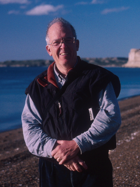
On Saturday, June 10, Dr. Roger Payne passed away. Throughout his remarkable life, he made impactful contributions to the study, understanding, and conservation of whales. His passion, research, and advocacy efforts played a pivotal role in reshaping public perception, and thus promoting the conservation of these giants, profoundly influencing generations of researchers in the field of conservation biology, including myself.
Roger in Patagonia where here found his love for Southern Right Whales. Credit: Dr. Mariano Sironi / ICB.
In 1970, Roger and his first wife Katy Paine began the Southern Right Whale (SRW) Research Program in Patagonia, Argentina, which in 1996 was continued by the Whale Conservation Institute of Argentina (the ICB) , becoming the longest continually running research program on a great whale (based on known individuals) in existence. In this study, Dr. Payne recognized that individual whales can be identified by the unique marks on their heads, establishing an important milestone for photo-ID, a technique that forms the bedrock of whale science.
I am proud to say that I am part of his legacy, as a member of the ICB. With the SRW program, I continued advancing research on SRW through my doctoral dissertation by advancing methods in conservation physiology (see blog post) to understand the underlaying mechanisms affecting young whales’ mortality in Patagonia (see blog post ).
Probably, one of the most remarkable contributions of Dr. Payne to the field and to whale conservation was his groundbreaking discovery of the humpback whale song. In the mid-20th century, the world’s whale populations were intensively killed by commercial whalers, threatening their extinction. In the late 1960s, Payne and his collaborators unveiled the melodic symphonies of humpback whales, marking the start of modern whale biology and catalyzing the global conservationist movement “Save the Whales”. These haunting songs connected humans with these enigmatic animals in an emotional manner, raising public opinion and support for whale conservation that ultimately led to the global moratorium on commercial whaling in 1982.
Listen to this story on NPR featuring Roger Payne’s LP, ‘Songs of the Humpback Whale,’ released in 1970, which played a pivotal role in sparking the global environmental movement “Save the Whales”, helping whale populations on the brink of extinction. Photo: Ocean Alliance.
While he continued to believe that science provides essential information about the necessary changes needed to protect whales, Dr. Payne strongly believe in that the paths to accelerate these changes often involve a combination of activism and creative arts.
“…All of the great movements in human history have been based not on data but on emotion and passion, and a dream of a better society and a better life. For unless people connect emotionally with a problem they won’t connect with the numbers and the data that describe its dimensions…”
“…It seems highly likely that the changes we so desperately need will only come by invoking emotions, and that is something that poets, musicians, writers, playwrights, sculptors, painters, dancers, composers—in fact, creative people of every stripe do well, but that scientists do at their peril. For the real challenge here is to get the world to fall so deeply in love with Nature that we will no longer tolerate the destruction of creation, and will risk our careers and our lives to save all plankton, mosses, ferns, trees, flowers, jellyfish, crinoids, nautiloids, crabs, bees, butterflies, beetles, squid, fishes, frogs, turtles, birds, and mammals—in other words, we will fight to save all of the non-human “Other”…”
Roger Payne’s influence and legacy continue to inspire generations of scientists and conservationists. His work expanded our understanding of whales, deepened our empathy for these creatures, and paved the way for international collaborations aimed at protecting marine life and preserving our oceans. Today, there are many of us who, inspired by Roger, dedicate our lives to research, environmental education, and conservation. And following Roger’s teachings, we constantly ask questions to seek answers that allow us to continue learning about whales in a changing world.
Did you enjoy this blog? Want to learn more about marine life, research, and conservation?
Subscribe to our blog and get a message when we post a new blog. Just add your name and email into the subscribe box below.
By Abby Tomita, undergraduate student, OSU College of Earth, Ocean, and Atmospheric Sciences, research intern in the GEMM and Krill Seeker Labs
This February, during the winter term of my third year at Oregon State, I was presented with a once-in-a-lifetime opportunity. After spending the last year studying the zooplankton krill as part of Project OPAL, I was invited to spend the austral winter season doing research on Antarctic krill (Euphausia superba) under supervision of experts Dr. Kim Bernard and PhD student Rachel Kaplan. Additionally, we were lucky enough to participate in two research cruises along the Western Antarctic Peninsula (WAP).
Figure 1. Sailing into the sunset on the RV Laurence M. Gould.
Unsurprisingly, it is no easy feat getting to the bottom of the world. After an incredibly thorough physical qualification process and two days of air travel from Portland, Oregon, we reached the lovely city of Punta Arenas, Chile. It was such a relief to arrive – but we were only halfway there. The next portion of our trip was the one that I was most anxious about, especially as someone who is prone to seasickness: crossing the Drake Passage. This stretch of the ocean, from the southernmost tip of South America to the Antarctic Peninsula, is notoriously treacherous as water in this area circulates the globe completely unobstructed by land masses. I soon learned the value of scopolamine patches and nausea bracelets, which helped me immensely through this five day journey. From Punta Arenas, we boarded the RV Laurence M. Gould, along with a seal research team from the University of North Carolina Wilmington. They were headed down south to look for crabeater seals to better understand not only their physiology, but also their role in the trophic ecology of the WAP.
The Passage was rough, but not as terrible as I expected. The hype around it made me think I’d be faced with something as menacing as the giant wave from The Perfect Storm, and while the rocking and rolling of the ship was far from pleasant, my nausea aids, as well as the amazing people and vast selection of movies on board made it manageable. Despite being extremely nervous for the Passage, I was also very excited to celebrate my twenty-first birthday during it. It was a memorable, although untraditional birthday experience that was made all the more special by my friends on the ship who took the time to celebrate the day as best as we could.
Figure 2. Taking in the sights of the Neumayer Channel with Kim!
The morning that we reached the Bransfield Strait was something truly unforgettable. Up until that point, I knew our destination was Antarctica, but I couldn’t really wrap my head around it because it was such a distant place and concept to me. I remember walking out onto the starboard side of the second level deck and seeing huge mountains out in the distance. For some reason, I had never considered how massively tall the mountains of the peninsula are, and just the fact that there were mountains down here at all. I joined the others at the bow, where we stood for hours in awe at the first land we had seen in days. Though many of the other scientists and crew members on board had been to this icy continent before, this was my first time, and I was in a state of disbelief. We’d finally made it and it sunk into me that I was in Antarctica, and that I would be here for the next five and half months.
After a day of hiding from strong winds in the Neumayer Channel, we were able to dock at Palmer Station (the smallest of the three US research bases in Antarctica) for our first port call, and seeing Palmer for the first time was just as exciting as seeing the continent. It looked so small at first, especially with the glacier and mountains looming behind it. Once the ship was tied up, orientation began. The station manager came onto the ship to give us an overview of what we could expect on station and the general Palmer etiquette. Next, we were given a tour of the facilities, from the lab spaces and aquarium room, up through the galley/dining area, past the hot tub and sauna, and into the lounge and bar in the GWR (Garage, Warehouse, and Recreation) building. I was surprised at how cozy the station was on the inside. In pictures, the buildings’ exteriors looked similar to the outside of a metal shipping container, but the inside was welcoming and warm. Those of us staying on station then sat through several hours of a more detailed orientation that somehow wore us out despite sitting in comfy recliner sofas the whole time. After sleeping on the rocking ship for about a week, I had some of the best sleep of my life that first night at Palmer Station.
Figure 3. Arriving at the Palmer Station pier in the first morning light.
Our first research cruise started a few days after arriving at Palmer, and just like that, we were off to explore the Southern Ocean. This leg of the trip took us south, down to Marguerite Bay and the region of Alexander Island, for ten days. The views were just spectacular everywhere we went, and it was so humbling to step out onto the deck to see gigantic mountains all around the ship. By day, us “krillers”, as our team is known, camped out on the bridge of the ship with the seal team, where we looked for sea ice floes with lounging crabeater seals. By night we conducted CTD casts, filtered water for chlorophyll, and deployed nets to catch our favorite tiny crustacean critters, along with any other zooplankton in our track. Unfortunately for both our group and the seal team, many areas that we visited were not frequented by krill or crabeater seals, though the seal team did successfully study and tag one seal over the course of the first cruise.
Figure 4. Rachel (right) and I (left) filtering water for chlorophyll on the LMG.
One of the highlights of this leg of the cruise was our Crossing Ceremony, as we’d crossed the Antarctic Circle (approximately 66.5ºS) shortly after leaving Palmer station. Myself and six others were crossing for the first time, so to earn our “Red Noses”, we had to pay tribute to King Neptune and his court. It would not be a Crossing Ceremony without at least some light pranking, so when they brought us out individually to the main deck, I knew something was coming our way.
Figure 5. Taking a celebratory picture with King Neptune’s court…with a surprise after.
The ten days flew by, and when we arrived back on station, we had less than a week to prepare for our next excursion on the LMG, which would be fifteen days. The time back at Palmer went quickly as we organized our lab space and entered data from the first cruise. The ship came back once more and we were off, this time heading north along the Peninsula to the Gerlache Strait. The sights were as breathtaking as ever, and I was excited to be back with my friends from the ship.
Figure 6. Kim (left) and I (right) pour krill we caught into an XACTIC tank.
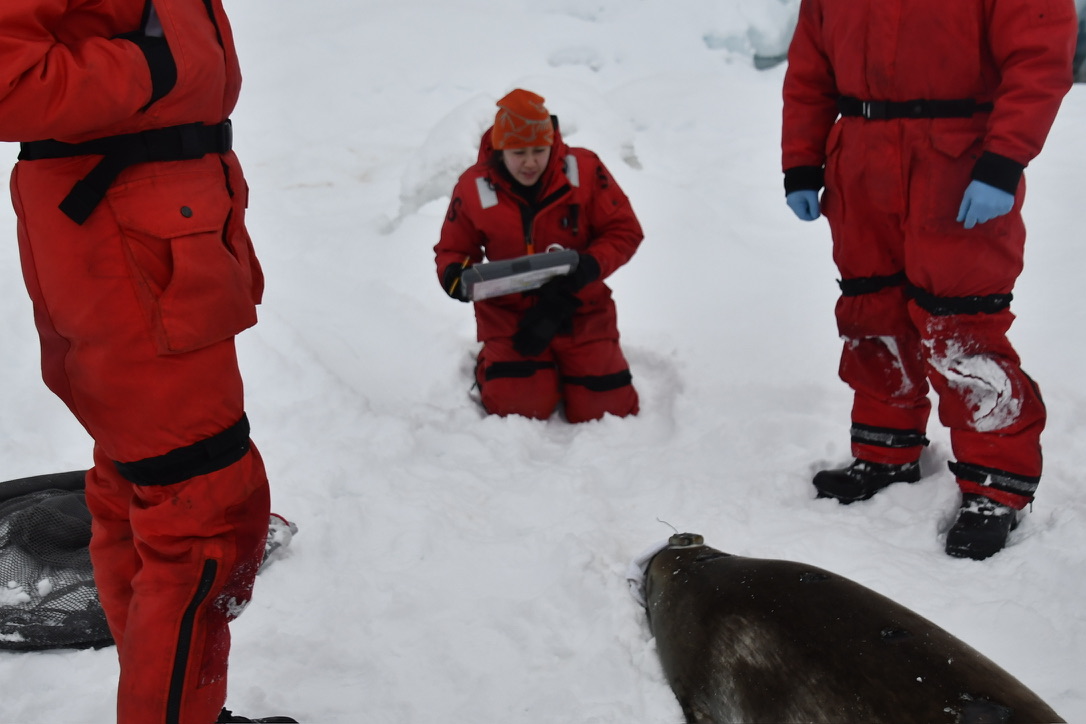
Our first day of transit was through the Lemaire Channel, one of the most stunning areas that we passed through (check out the photo gallery at the end of this post!). We spent the majority of the day on the bow and the deck of the bridge taking in the beautiful towering mountains on either side of the narrow channel and watching for penguins and humpbacks, of which there were many. This voyage segued into an extremely productive night of science for us where we caught thousands of krill that we were able to keep live in tanks on the ship, in preparation for later use for our experiments on station. Our first productive night of science was auspicious for the rest of the cruise as we caught and processed thousands more krill, and the seal team had a much more fruitful experience finding crabeater seals (they found/worked on 8 seals and named them all after fruits!). The highlight of this second cruise for me was getting to accompany the seal team onto an ice floe in the Lemaire Channel to assist them in their work on the crabeater, a female juvenile who they named Mango!
Figure 7. Watching Mango’s nose to calculate and record her breaths per minute (US NMSF Permit #25770).
Returning to Palmer for the final time on the LMG was just as exciting as arriving the first time, especially with the knowledge that we’d have one last night of celebration with our friends from the ship at the Cross Town Dinner – a night to celebrate the solstice with both the Palmer crew and LMG crew. Although the dinner and subsequent party were a blast, I felt a lingering sadness knowing that the majority of the people I spent almost two months with would be heading north, back to their respective homes while Kim, Rachel, and I stayed at Palmer for the next few months. The next day, after saying our goodbyes, the three of us stood on the Palmer pier with tears streaming down our faces, waving frantically at the ship to our friends on the deck. In spite of my sadness, I knew that the coming months would be a thrilling series of new experiences in one of the most magical and special places that I have ever had the pleasure of being in.
Figure 8. The LMG departs Palmer Station for the last time this winter!
By Morgan O’Rourke-Liggett, M.S., Oregon State University, Department of Fisheries, Wildlife, and Conservation Sciences, Geospatial Ecology of Marine Megafauna Lab
It is the end.
I graduated with a Master’s degree.
This journey began 10 years ago when I visited colleges as a high school junior.
Begin with the end in mind.
I knew I would major in science as an undergrad and focus on something more specific as a graduate student. Studying whales required a background in marine biology, which led to my undergraduate degree in oceanography with strong emphasis in fisheries and wildlife, policy, and ecology. My master’s degree was built on that and added specific skills in data collection, management, and analysis.
The last time I wrote a blog, I was sharing the details of the data management and intricacies of my master’s project. Part of what made that project so successful was knowing the end goal: we wanted to know the area surveyed based on visibility and a visual representation of it. This knowledge aided in the development of matrices for environmental conditions, assigning integer variables to text survey notes, and determining what toolboxes and packages would be the most appropriate for analysis.
As a visual learner, I like to sketch out what I am doing or draw it on a whiteboard in a concept board. This approach is something I have always done and was further reinforced as a necessary step in my programming classes early on in my master’s education. My professors would assign a problem that could be solved in programming by making a function or script of code. We were taught to write out what our end goals were and what inputs were available for the problem. From there, filling in what steps were needed would be added. That was a critical step that made writing many difficult Python and R for loops and functions easier to build.
This skill and mentality of “beginning with the end” in mind can also be useful in preparation for data collection. There are eleven common data types that are described with examples in Table 1. Understanding what data type is being collected could save several hours of data management and wrangling during the data analysis phase. From my experience in data analytics, some models yield more accurate results if the character data is manipulated to behave like an integer in R. Additionally, certain packages and toolboxes in R and GIS are only useful for certain data types.
Data Type
Definition
Example
Integer (int)
Numeric data without fractions
-707, 0, 707
Floating point (float) or Double
Numeric data with fractions
707.07, 0.7, 707.00
Character (char)
Single letter, digit, space, punctuation mark, symbol
a, !
String (str or text) or Complex
Sequence of characters, digits, or symbols
Hello, +1-999-666-3333
Boolean (bool) or Logical
True or false values
0 (false), 1 (true)
Enumerated type (enum)
Small set of predefined values that can be text or numerical
rock (0), jezz (1)
Array
List with a number of elements in a specific order
rock (0), jazz (1), blues (2), pop (3)
Data
Date in YYYY-MM-DD fomat
2021-09-28
Time
Time in hh:mm:ss format or a time interval between two events
12:00:59
Datetime
Stores a value of both YYYY-MM-DD hh:mm:ss
2021-09-28 12:00:59
Timestamp
Number of seconds that have elapsed since midnight, 1st January 1970 in UTC
1632855600
Table 1. Table of the eleven most common data types with a short definition and an example of the data type. Table inspired by (Choudhury 2022).
Beginning with the end in mind allows more clarity and strategies to be efficient and achieve your goal. It develops a better understanding of why each stage of data collection and analysis is important; why each stage in a career is important. It provides a road map for what will, undoubtedly, be an incredible learning experience.
Did you enjoy this blog? Want to learn more about marine life, research, and conservation? Subscribe to our blog and get a weekly message when we post a new blog. Just add your name and email into the subscribe box below.
The winds are consistently (and sometimes aggressively) blowing from the north here on the Oregon coast, which can only mean one thing – summer has arrived! Since mid-May, the GRANITE (Gray whale Response to Ambient Noise Informed by Technology and Ecology) team has been looking for good weather windows to survey for gray whales and we have managed to get five great field work days already. In today’s blog post, I am going to share what (and who) we have seen so far.
On our first day of the field season, PI Leigh Torres, postdoc KC Bierlich and myself, were joined by a special guest: Dr. Andy Read. Andy is the director of the Duke University Marine Lab, where he also runs his own lab, which focuses on conservation biology and ecology of marine vertebrates. Andy was visiting the Hatfield Marine Science Center as part of the Lavern Weber Visiting Scientist program and was hosted here by Leigh. For those of you that do not know, Andy was Leigh’s graduate school advisor at Duke where she completed her Master’s and doctoral degrees. It felt very special to have Andy on board our RHIB Ruby for the day and to introduce him to some friends of ours. The first whale we encountered that day was “Pacman”. While we are always excited to re-sight an individual that we know, this sighting was especially mind-blowing given the fact that Leigh had “just” seen Pacman approximately two months earlier in Guerrero Negro, one of the gray whale breeding lagoons in Mexico (read this blog about Leigh and Clara’s pilot project there). Aside from Pacman, we saw five other individuals, all of which we had seen during last year’s field season.
The first day of field work for the 2023 GRANITE field season! From left to right: Leigh Torres, Lisa Hildebrand, Andy Read, and KC Bierlich. Source: L. Torres.
Since that first day on the water, we have conducted field work on four additional days and so far, we have only encountered known individuals in our catalog. This fact is exciting because it highlights the strong site fidelity that Pacific Coast Feeding Group (PCFG) gray whales have to areas within their feeding range. In fact, I am examining the residency and space use of each individual whale we have observed in our GRANITE study for one of my PhD chapters to better understand the level of fidelity individuals have to the central Oregon coast. Furthermore, this site fidelity underpins the unique, replicate data set on individual gray whale health and ecology that the GRANITE project has been able to progressively build over the years. So far during this field season in 2023, we have seen 13 unique individuals, flown the drone over 10 of them and collected four fecal samples from two, which represent critical data points from early on in the feeding season.
Our sightings this year have not only highlighted the high site fidelity of whales to our study area but have also demonstrated the potential for internal recruitment of calves born to “PCFG mothers” into the PCFG. Recruitment to a population can occur in two ways: externally (individuals immigrate into a population from another population) or internally (calves born to females that are part of the population return to, or stay, within their mothers’ population). Three of the whales we have seen so far this year are documented calves from females that are known to consistently use the PCFG range, including our central Oregon coast study area. In fact, we documented one of these calves, “Lunita”, just last year with her mother (see Clara’s recap of the 2022 field season blog for more about Lunita). The average calf survival estimate between 1997-2017 for the PCFG was 0.55 (Calambokidis et al. 2019), though it varied annually and widely (range: 0.34-0.94). Considering that there have been years with calf survival estimates as low as ~30%, it is therefore all the more exciting when we re-sight a documented calf, alive and well!
“Lunita”, an example of successful internal recruitment
We have also been collecting data on the habitat and prey in our study system by deploying our paired GoPro/RBR sensor system. We use the GoPro to monitor the benthic substrate type and relative prey densities in areas where whales are feeding. The RBR sensor collects high-frequency, in-situ dissolved oxygen and temperature data, enabling us to relate environmental metrics to relative prey measurements. Furthermore, we also collect zooplankton samples with a net to assess prey community and quality. On our five field work days this year, we have predominantly collected mysid shrimp, including gravid (a.k.a. pregnant) individuals, however we have also caught some Dungeness and porcelain crab larvae. The GEMM Lab is also continuing our collaboration with Dr. Susanne Brander’s lab at OSU and her PhD student Lauren Kashiwabara, who plan on conducting microplastic lab experiments on wild-caught mysid shrimp. Their plan is to investigate the growth rates of mysid shrimp under different temperature, dissolved oxygen, and microplastic load conditions. However, before they can begin their experiments, they need to successfully culture the mysids in the lab, which is why we collect samples for them to use as their ‘starter culture’. Stay tuned to hear more about this project as it develops!
So, all in all, it has been an incredibly successful start to our field season, marked by the return of many familiar flukes and flanks! We are excited to continue collecting rock solid GRANITE data this summer to increase our efforts to understand gray whale ecology and physiology.
References
Calambokidis, J., Laake, J., and Perez, A. (2019). Updated analyses of abundance and population structure of seasonal gray whales in the Pacific Northwest, 1996-2017. IWC, SC/A17/GW/05 for the Workshop on the Status of North Pacific Gray Whales. La Jolla: IWC.
By Annie Doron, Undergraduate Intern, Oregon State University, GEMM Laboratory
Hey up! My name is Annie Doron, and I am an undergraduate Environmental Science student from the University of Sheffield (UK) on my study year abroad. One of my main motivations for undertaking this year abroad was to gain experience working in a marine megafauna lab. Whales in particular have always captivated my interest, and I have been lucky enough to observe humpback whales in Iceland and The Azores, and even encountered one whilst diving in Australia! For the past 10 months, I have had the unique opportunity to work in the GEMM Lab analyzing Pacific Coast Feeding Group (PCFG) gray whales off the Oregon Coast (Figure 1). I must admit, it has been simply wonderful!
Figure 1. Aerial image of a PCFG gray whale off the Oregon Coast.
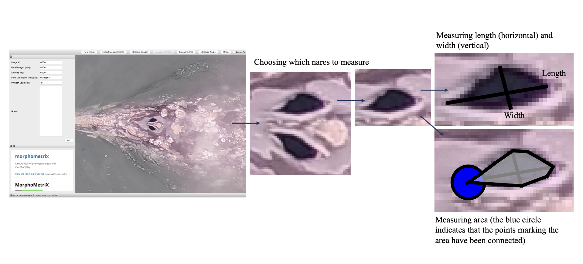
How did I end up getting involved with the GEMM Lab? I was first accepted into Scarlett Arbuckle’s research-based class in fall term 2022, which is centered around partnering with a mentor for a research project. Having explored the various fields of research at HMSC, I contacted Leigh Torres with interest in getting involved in the GEMM Lab and to establish a research project suitable for a totally inexperienced, international, undergraduate student. Thankfully, Leigh forwarded my email to KC Bierlich who offered to be my mentor for the class, and the rest is history! I first began analyzing drone imagery to measure length and body condition of PCFG gray whales, which provided an opportunity to get involved with the lab and gain experience using the photogrammetry software MorphoMetriX (Torres & Bierlich, 2020) (see KC’s blog), which is used to make morphometric measurements of whales. Viewing drone imagery of whales sparked my interest in how they use their blowholes (otherwise called ‘nares’) to replenish their oxygen stores; this led to us establishing a research project for the class where we tested if we could use MorphoMetriX to measure blowholes from drone imagery.
Extending this project into winter and spring terms (via research credits) has enabled me to continue working with Leigh and KC, as well as to collaborate with Clara Bird and Jim Sumich. Thanks to KC, who has patiently guided me through the ins and outs of working on a research project, I now feel more confident handling and manipulating large datasets, analyzing drone footage (i.e., differentiating between behavioral states, recording breathing sequences, detecting when a whale is exhaling vs inhaling, etc.), and speaking in public (although I still get pretty bad stage fright, but I think that is a typical conundrum undergrads face). Whatsmore, applying R – a programming language used for statistical analysis and data visualization, which I have been trying to wrap my head around for years – to my own dataset has helped me greatly enhance my skills using it.
So, what exciting things have we been working on this year? Given that we often cannot simply study a whale from inside a laboratory – due to size-related logistical implications – we must use proxies (i.e., a variable that is representative of an immeasurable variable). Since cetaceans must return to the surface to offload carbon dioxide and replenish their oxygen stores, measuring their breath frequency and magnitude is one way to study a whale’s oxygen consumption, in turn offering insight into its energy expenditure (Williams, 1999). Blowholes are one proxy we can use to study breath magnitude. Blowholes can be utilized in this way by measuring inhalation duration (the amount of time a whale is inhaling, which is based on a calculation developed by Jim Sumich) and blowhole area (the total area of a blowhole) to gauge variations in tidal volume (the amount of air flowing in and out of the lungs).
Measuring inhalation duration and blowhole area is important because a larger blowhole area (i.e., one that is more dilated) and a longer inhalation duration is indicative of higher oxygen intake, which can infer stress. For example, in this population, higher stress levels are associated with increased vessel traffic (Lemos et al., 2022), and skinnier whales have higher stress levels compared to chubby, healthy whales (Lemos, Olsen, et al., 2022). Hence, measuring the variation around blowholes could be utilized to predict challenges whales face from climate change and anthropogenic disturbance, including fishing (Scordino et al., 2017) and whale watching industry threats (Sullivan & Torres, 2018) (see Clara’s blog), as well as to inform effective management strategies. Furthermore, measuring the variables inhalation duration and blowhole area could help to identify whether whales are taking larger breaths associated with certain ‘gross behavior states’, otherwise known as ‘primary states’, which include: travel, forage, rest, social (Torres et al., 2018). This could enable us to assess the energetic costs of different foraging tactics (i.e., head standing, side-swimming, and bubble blasting (Torres et al., 2018), as well as consequences of disturbance events, on an individual and population health perspective.
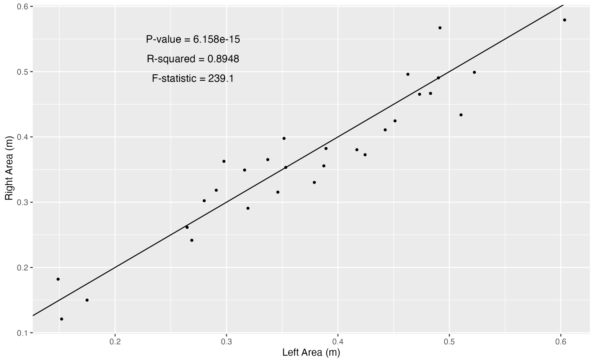
Inhalation duration has been explored in the past by using captive animals. For example, there have been studies on heart rate and breathing of bottlenose dolphins in human care facilities (Blawas et al., 2021; Fahlman et al., 2015). Recently, Nazario et al. (2022) was able to measure inhalation duration and blowhole area using suction-cup video tags. Her study led us to consider if it was possible to measure the parameters and variation around respiration by measuring blowhole area and inhalation duration of PCFGs from drone imagery. We employed MorphoMetriX to study the length, width, and area of a blowhole (Figure 2). Preliminary analyses verified that the areas of the left and right blowholes are very similar (Figure 3); this finding saved us a lot of time because from thereon we only measured either the left or right side. Interestingly, we see some variation in blowhole area within and across individuals (Figure 4). This variation changes within individuals based on primary state. For example, the whales “Glacier”, “Nimbus”, and “Rat” show very little variation whilst traveling but a large amount whilst foraging. Comparatively, “Dice” shows little variation whilst foraging and large variation whilst traveling. Whilst considering cross-individual comparisons, we can see that “Sole”, “Rat”, “Nimbus”, “Heart”, “Glacier”, “Dice”, and “Coal” each exhibit relatively large amounts of variation, yet “Mahalo”, “Luna”, “Harry”, “Hummingbird” and “Batman” exhibit very little. One potential reason for some individuals displaying higher levels of variation than others could be higher levels of exposure to disturbance events that we were unable to measure or evaluate in this study.
Figure 2. How we measured the length, width, and area of a blowhole using MorphoMetriX.
Figure 3. Data driven evidence that the left and the right blowhole areas are very similar.
Figure 4. Variation in blowhole area amongst individual PCFG whales. The hollow circles represent the means, and the color represents the primary state the whale is exhibiting, foraging (purple) vs. traveling (blue), which will be further explored in Clara’s PhD.
Now, we are venturing into June and are at a stage where we (KC, Clara, Jim, Leigh, and I) are preparing to publish a manuscript! What a way to finish such a fantastic year! The transition from a 3-month-long pilot study to a much larger data analysis and eventual preparation for a manuscript has been a monumental learning experience. If anybody had told me a year ago that I would be involved in publishing a body of work – especially one that is so meaningful to me – I would simply not have believed them! We hope this established methodology for measuring blowholes will help other researchers carry out blowhole measurements using drone imagery across different populations and species. Further research is required to explore the differences in inhalation duration and blowhole area between different primary states, specifically across different foraging tactics.
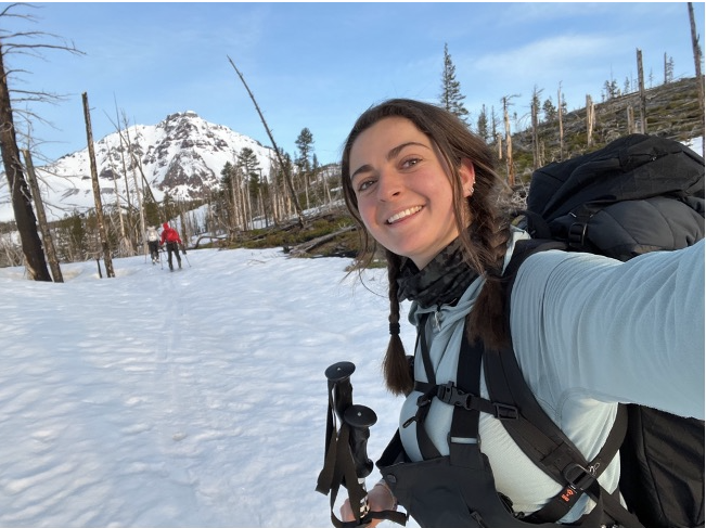
It has been a great privilege working with the GEMM Lab these past months, and I was grateful to be included in their monthly lab meetings, during which members gave updates and we discussed recently published papers. Seeing such an enthusiastic, kind, and empathic group of people working together taught me what working in a supportive lab could look and feel like. In spite of relocating from Corvallis to Bend after my first term, I was happy to be able to continue working remotely for the lab for the remainder of my time (even though I was ~200 miles inland). I thoroughly enjoyed living in Corvallis, highlights of which were scuba diving adventures to the Puget Sound and coastal road trips with friends. The appeal to move arose from Bend’s reputation as an adventure hub – with unlimited opportunities for backcountry ski access – as well as its selection of wildlife ecology courses (with a focus on species specific to central Oregon). I moved into ‘Bunk & Brew’ (Bend’s only hostel, which is more like a big house of friends with occasional hostel guests) on January 1st after returning from spending Christmas with friends in my old home in Banff, Canada. I have since been enjoying this wonderful multifaceted lifestyle; working remotely in the GEMM Lab, attending in-person classes, working part-time at the hostel, as well as skiing volcanoes (Mount Hood, Middle and South Sister (Figure 5) or climbing at Smith Rock during my days off. Inevitably, I do miss the beautiful Oregon coast, and I will always be grateful for this ideal opportunity and hope this year marks the start of my marine megafauna career!
Figure 5. What I get up to when I’m not studying blowholes! (This was taken at 5am on the long approach to Middle and North Sister. North Sister is the peak featured in the backdrop).
References
Blawas, A. M., Nowacek, D. P., Allen, A. S., Rocho-Levine, J., & Fahlman, A. (2021). Respiratory sinus arrhythmia and submersion bradycardia in bottlenose dolphins (Tursiops truncatus). Journal of Experimental Biology, 224(1), jeb234096. https://doi.org/10.1242/jeb.234096
Fahlman, A., Loring, S. H., Levine, G., Rocho-Levine, J., Austin, T., & Brodsky, M. (2015). Lung mechanics and pulmonary function testing in cetaceans. Journal of Experimental Biology, 218(13), 2030–2038. https://doi.org/10.1242/jeb.119149
Lemos, L. S., Haxel, J. H., Olsen, A., Burnett, J. D., Smith, A., Chandler, T. E., Nieukirk, S. L., Larson, S. E., Hunt, K. E., & Torres, L. G. (2022). Effects of vessel traffic and ocean noise on gray whale stress hormones. Scientific Reports, 12(1), 18580. https://doi.org/10.1038/s41598-022-14510-5
Lemos, L. S., Olsen, A., Smith, A., Burnett, J. D., Chandler, T. E., Larson, S., Hunt, K. E., & Torres, L. G. (2022). Stressed and slim or relaxed and chubby? A simultaneous assessment of gray whale body condition and hormone variability. Marine Mammal Science, 38(2), 801–811. https://doi.org/10.1111/mms.12877
Nazario, E. C., Cade, D. E., Bierlich, K. C., Czapanskiy, M. F., Goldbogen, J. A., Kahane-Rapport, S. R., van der Hoop, J. M., San Luis, M. T., & Friedlaender, A. S. (2022). Baleen whale inhalation variability revealed using animal-borne video tags. PeerJ, 10, e13724. https://doi.org/10.7717/peerj.13724
Scordino, J., Carretta, J., Cottrell, P., Greenman, J., Savage, K., & Scordino, J. (2017). Ship Strikes and Entanglements of Gray Whales in the North Pacific Ocean. Cambridge: International Whaling Commission, 1924–2015.
Sullivan, F. A., & Torres, L. G. (2018). Assessment of vessel disturbance to gray whales to inform sustainable ecotourism: Vessel Disturbance to Whales. The Journal of Wildlife Management, 82(5), 896–905. https://doi.org/10.1002/jwmg.21462
Sumich, J. L. (1994). Oxygen extraction in free-swimming gray whale caves. Marine Mammal Science, 10(2), 226–230. https://doi.org/10.1111/j.1748-7692.1994.tb00266.x
Torres, W., & Bierlich, K. (2020). MorphoMetriX: A photogrammetric measurement GUI for morphometric analysis of megafauna. Journal of Open Source Software, 5(45), 1825. https://doi.org/10.21105/joss.01825
Torres, L. G., Nieukirk, S. L., Lemos, L., & Chandler, T. E. (2018). Drone Up! Quantifying Whale Behavior From a New Perspective Improves Observational Capacity. Frontiers in Marine Science, 5, 319. https://doi.org/10.3389/fmars.2018.00319 Williams, T. M. (1999). The evolution of cost efficient swimming in marine mammals: Limits to energetic optimization. Philosophical Transactions of the Royal Society of London. Series B: Biological Sciences, 354(1380), 193–201. https://doi.org/10.1098/rstb.1999.0371
This year, for the 15th consecutive summer, the Hatfield Marine Science Center (HMSC) will be hosting undergraduate interns as part of the NSF-funded Research Experiences for Undergraduate (REU) program. The GEMM Lab will provide research experiences to no less than three REU interns for a 10-week period starting mid-June. Along with Leigh, Dawn, and Allison, I will be a daily “mentor” to one of these students; a role that the HMSC REU program takes very seriously.
I used quotation marks here because although I have been supervising/helping/engaging/leading teams and students for many years, I only really learned this new word, “mentoring”, after moving to the US. In my native language, French, the word “mentor” exists and has the same meaning as in English (i.e. a person who gives a younger or less experiencedpersonhelp and advice over a period of time, especially at work or school; Cambridge Dictionary). However, the verb derived from this noun – “mentoring” – does not exist in French and the word we use instead sounds more like “supervising”. Actually, an advisor to a trainee or intern is often called “maître de stage”, literally meaning “internship master”, which conveys a pretty different message from the title mentor…
Why does that semantic nuance matter? Well, I believe that the words we use are an extension of the way we see the world. Fact is, although I have been an advisor to several students before, I had never received any formal mentoring training up to today and I never put that much thought into what mentoring meant to me. Well, I certainly did not see myself being anyone’s Master! So, what is the difference between mentoring and supervising?
A quick google search gave me a hint… supervision is very much task-oriented, it’s about overseeing a person’s activities and providing instructions and recommendations to ensure that the task is successfully completed. That’s all good and well, but mentoring adds an additional layer of care for the person’s long-term development, in an approach that strives to be more holistic. That approach may seem obvious to many academics today, but unfortunately things don’t always happen that way. Many of us could cite several cases where we have observed students being used as additional work force without much attention given to their wellbeing, learning, and personal development. Who has never seen a real-life professor like that of Phd Comics (Illustration below)? On top of that, mentoring styles, and the academic system as a whole, have long shaped the new generations of scientists to resemble their senior mentors, hence perpetuating inequity in education and a lack of diversity in research carriers.
PhD Comics is probably one of the most hilarious yet highly accurate depictions of the flaws of academic mentoring. Comic reproduced from “Piled Higher and Deeper” by Jorge Cham, www.phdcomics.com.
I discovered that there are a lot of great resources out there to help early-career scientists navigate the waters of mentorship (e.g., Center for Improved Mentored Experiences in Research, OSU guidance for DEI learning). I also really appreciated the fact that the HMSC REU program director, Itchung Cheung, would take the time to meet all future mentors ahead of time, and make sure that they had the tools and resources to be good mentors. He made it clear that a student has many mentoring needs (e.g., role models, emotional support, access to opportunities, professional development…) and that it is not possible for one person to fill all these shoes. As PhD student Rachel Kaplan pointed out “It takes a village to raise a PhD student”! That being said, there are a couple simple rules that everyone should agree on before taking on interns or new students. I will not list all these best practices here but some of main take-away messages for me were the importance of planning, having clear expectations while staying flexible, encouraging interns to take an active role in setting goals and providing critical feedback, and fostering a welcoming environment in which the student can feel a sense of belonging.
Along those lines, I would like to end on a more personal note. Although I never received formal mentorship training, I do believe that I learned some of these skills in the most traditional way; that is by learning by example. And (hopefully!) this process did not turn too badly because I was lucky to have great mentors to look up to. Among other qualities, my mentors always made me feel like I belonged, like what I had to say mattered. Reflecting upon my years as a graduate student, I now realize that this feeling is one of the things that allowed me to love research, with all its setbacks and challenges. My mentors always made me feel like I was among their priorities, whether it be by returning manuscript edits in time or listening to me present all of my latest analysis outputs and coding tribulations. Holistic mentoring is a bit of a jargony word, and although I am still learning the theories underlying that approach, I know that if that’s what I experienced as a mentee, then that’s what I will try to do as a mentor!
To learn more about research experiences for undergraduate at Oregon State University, check out this link.
Recently, I had the opportunity to attend the Effects of Climate Change on the World’s Ocean (ECCWO) conference. This meeting brought together experts from around the world for one week in Bergen, Norway, to gather and share the latest information on how oceans are changing, what is at risk, responses that are underway, and strategies for increasing climate resilience, mitigation, and adaptation. I presented our recent findings from the EMERALD project, which examines gray whale and harbor porpoise distribution in the Northern California Current over the past three decades. Beyond sharing my postdoctoral research widely for the first time and receiving valuable feedback, the ECCWO conference was an incredibly fruitful learning experience. Marine mammals can be notoriously difficult to study, and often the latest methodological approaches or conceptual frameworks take some time to make their way into the marine mammal field. At ECCWO, I was part of discussions at the ground floor of how the scientific community can characterize the impacts of climate change on the ecosystems, species, and communities we study.
One particular theme became increasingly apparent to me throughout the conference: as the oceans warm, what are “anomalous conditions”? There was an interesting dichotomy between presentations focusing on “extreme events,” “no-analog conditions,” or “non-stationary responses,” compared with discussions about the overall trend of increasing temperatures due to climate change. Essentially, the question that kept arising was, what is our frame of reference? When measuring change, how do we define the baseline?
Marine heatwaves have emerged as an increasingly prevalent phenomenon in recent years (see previous GEMM Lab blogs about marine heatwaves here and here). The currently accepted and typically applied definition of a marine heatwave is when water temperatures exceed a seasonal threshold (greater than the 90th percentile) for a given length of time (five consecutive days or longer) (Hobday et al. 2016). These marine heatwaves can have substantial ecosystem-wide impacts including changes in water column structure, primary production, species composition, distribution, and health, and fisheries management such as closures and quota changes (Cavole et al. 2016, Oliver et al. 2018). Through some of our own previous research, we documented that blue whales in Aotearoa New Zealand shifted their distribution (Barlow et al. 2020) and reduced their reproductive effort (Barlow et al. 2023) in response to marine heatwaves. Concerningly, recent projections anticipate an increase in the frequency, intensity, and duration of marine heatwaves under global climate change (Frölicher et al. 2018, Oliver et al. 2018).
However, as the oceans continue to warm, what baseline do we use to define anomalous events like marine heatwaves? Members of the US National Oceanic and Atmospheric Administration (NOAA) Marine Ecosystem Task Force recently put forward a comment article in Nature, proposing revised definitions for marine heatwaves under climate change, so that coastal communities have the clear information they need to adapt (Amaya et al. 2023). The authors posit that while a “fixed baseline” approach, which compares current conditions to an established period in the past and has been commonly used to-date (Hobday et al. 2016), may be useful in scenarios where a species’ physiological limit is concerned (e.g., coral bleaching), this definition does not incorporate the combined effect of overall warming due to climate change. A “shifting baseline” approach to defining marine heatwaves, in contrast, uses a moving window definition for what is considered “normal” conditions. Therefore, this shifting baseline approach would account for long-term warming, while also calculating anomalous conditions relative to the current state of the system.
An overview of two different definitions for marine heatwaves, relative to either fixed or shifting baselines. Reproduced from Amaya et al. 2023.
Why bother with these seemingly nuanced definitions and differences in terminology, such as fixed versus shifting baselines for defining marine heatwave events? The impacts of these events can be extreme, and potentially bear substantial consequences to ecosystems, species, and coastal communities that rely on marine resources. With the fixed baseline definition, we may be headed toward perpetual heatwave conditions (i.e., it’s almost always hotter than it used to be), at which point disentangling the overall warming trends from these short-term extremes becomes nearly impossible. What the shifting baseline definition means in practice, however, is that in the future temperatures would need to be substantially higher than the historical average in order to qualify as a marine heatwave, which could obscure public perception from the concerning reality of warming oceans. Yet, the authors of the Nature comment article claim, “If everything is extremely warm all of the time, then the term ‘extreme’ loses its meaning. The public might become desensitized to the real threat of marine heatwaves, potentially leading to inaction or a lack of preparedness.” Therefore, clear messaging surrounding both long-term warming and short-term anomalous conditions are critically important for adaptation and resource allocation in the face of rapid environmental change.
While the findings presented and discussed at an international climate change conference could be considered quite disheartening, I left the ECCWO conference feeling re-invigorated with hope. Crown Prince Haakon of Norway gave the opening plenary and articulated that “We need wise and concerned scientists in our search for truth”. Later in the week, I was a co-convenor of a session that gathered early-career ocean professionals, where we discussed themes such as how we deal with uncertainty in our own climate change-related ocean research, and importantly, how do we communicate our findings effectively. Throughout the meeting, I had formal and informal discussions about methods and analytical techniques, and also about what connects each of us to the work that we do. Interacting with driven and dedicated researchers across a broad range of disciplines and career stages gave me some renewed hope for a future of ocean science and marine conservation that is constructive, collaborative, and impactful.
Enjoying the ~anomalously~ sunny April weather in Bergen, Norway, during the ECCWO conference.
Now, as I am diving back in to understanding the impacts of environmental conditions on harbor porpoise and gray whale habitat use patterns through the EMERALD project, I am keeping these themes and takeaways from the ECCWO conference in mind. The EMERALD project draws on a dataset that is about as old as I am, which gives me some tangible perspective on how things have things changed in the Northern California Current during my lifetime. We are grappling with what “anomalous” conditions are in this dynamic upwelling system on our doorstep, whether these anomalies are even always bad, and how conditions continue to change in terms of cyclical oscillations, long-term trends, and short-term events. Stay tuned for what we’ll find, as we continue to disentangle these intertwined patterns of change.
Did you enjoy this blog? Want to learn more about marine life, research, and conservation? Subscribe to our blog and get a weekly alert when we make a new post! Just add your name into the subscribe box below!
References
Amaya DJ, Jacox MG, Fewings MR, Saba VS, Stuecker MF, Rykaczewski RR, Ross AC, Stock CA, Capotondi A, Petrik CM, Bograd SJ, Alexander MA, Cheng W, Hermann AJ, Kearney KA, Powell BS (2023) Marine heatwaves need clear definitions so coastal communities can adapt. Nature 616:29–32.
Barlow DR, Bernard KS, Escobar-Flores P, Palacios DM, Torres LG (2020) Links in the trophic chain: Modeling functional relationships between in situ oceanography, krill, and blue whale distribution under different oceanographic regimes. Mar Ecol Prog Ser 642:207–225.
Barlow DR, Klinck H, Ponirakis D, Branch TA, Torres LG (2023) Environmental conditions and marine heatwaves influence blue whale foraging and reproductive effort. Ecol Evol 13:e9770.
Cavole LM, Demko AM, Diner RE, Giddings A, Koester I, Pagniello CMLS, Paulsen ML, Ramirez-Valdez A, Schwenck SM, Yen NK, Zill ME, Franks PJS (2016) Biological impacts of the 2013–2015 warm-water anomaly in the northeast Pacific: Winners, losers, and the future. Oceanography 29:273–285.
Frölicher TL, Fischer EM, Gruber N (2018) Marine heatwaves under global warming. Nature 560.
Hobday AJ, Alexander L V., Perkins SE, Smale DA, Straub SC, Oliver ECJ, Benthuysen JA, Burrows MT, Donat MG, Feng M, Holbrook NJ, Moore PJ, Scannell HA, Sen Gupta A, Wernberg T (2016) A hierarchical approach to defining marine heatwaves. Prog Oceanogr.
Oliver ECJ, Donat MG, Burrows MT, Moore PJ, Smale DA, Alexander L V., Benthuysen JA, Feng M, Sen Gupta A, Hobday AJ, Holbrook NJ, Perkins-Kirkpatrick SE, Scannell HA, Straub SC, Wernberg T (2018) Longer and more frequent marine heatwaves over the past century. Nat Commun 9:1–12.
While I did not mean to start a mini-blog series on individual specialization, here I am with my third blog about individual specialization in as many years. Looking back, these blogs are actually a lovely documentation of my own journey of learning about individual specialization and I hope you’re enjoying being along for the ride.
So, what have we learned so far? In my first blog I described the concept of individual specialization, why it matters, and presented some case studies. In my second blog I discussed the roles of competition and learning as drivers of individual specialization. Let’s review: Individual specialization is when individuals within a population only use a subset of the resources that the full population uses, but different individuals use different subsets. This is important to quantify for two reasons: (1) it affects how we think about conserving and managing a population (Bolnick et al., 2003), and (2) it can affect the relationships between the population and the other species in its community (Bolnick et al., 2011). Common drivers of specialization are competition and learning. Competition can lead to specialization because it reduces the availability of a resource, driving individuals to switch resource use (Pianka, 1974). Learning can also lead to specialization through ‘one-to-one’ learning, where one individual learns from one demonstrator (Sheppard et al., 2018). This individual tends to then use, and eventually teach, that specialized technique.
While understanding these drivers is important, the question of why specific individuals employ specific specializations remains. If learning is not the driver of specialization, then how do individuals end up using their specific subset. Is it random? Or are there underlying patterns? The common sources of variation are related to sex, age, or size (and often these three can be inter-connected) (Dall et al., 2012).
Individual differences related to the sex of the individuals are called sexual dimorphisms. Physical and ecological differences between the sexes are common throughout nature (peacocks for example) and these differences can lead to different specializations. Northern elephant seals provide a fascinating example (Kienle et al., 2022). Northern elephant seal males are the distinctly larger sex as they engage in competitionfor females. Because of their larger body size and energy expenditure during competition, they have much higher energetic requirements than females during the breeding season, meaning that they need to consume more prey. This elevated requirement has led to a difference in foraging behaviors. Males forage near the continental shelf where there is more prey while females forage further offshore in the open ocean. However, the tradeoff of feeding on the continental shelf is an increased predation risk due to overlap with predator habitat, and indeed Kienle et al. found that the mortality rate for foraging trips was 5-6 times higher for males than females. So, while males need to take the risk of foraging in an area with higher predator presence to meet their energetic demands, females can forage in a safer habitat with less prey because their energetic requirements are lower. This study presents an excellent example of how sexual dimorphism can cause individual specialization and the subsequent consequences.
Individual specializations attributed to differences between distinct morphs are called resource polymorphisms. A morph is the physical appearance of an individual; distinct morphs are when there are clearly different kinds of morphs within a population. Morphs can range from color polymorphism (ex. lizards of different colors within the same species) to differences in skull shape and size. A study on the European eel found that differences in skull morphology were related to different foraging strategies (Cucherousset et al., 2011). Eels with larger head widths consumed larger prey types. Interestingly, they found that eels on either end of the head width spectrum (i.e., very narrow or very wide) were more successful (i.e., in better body condition) than eels with intermediate head widths. They suggest that this difference in nutrition success is because the intermediate head width eels were less efficient foragers than eels at the extremes. In this example we see that morphology is related to the ability to feed on a prey type and has consequences for individual health.
Figure 2. from Cucherousset et al., 2011. Small-bodied eels with narrower (a) and broader (b) heads and large-bodied eels with narrower (c) and broader (d) heads. TL (Total Length) and HW (Head Width):TL are shown for each individual
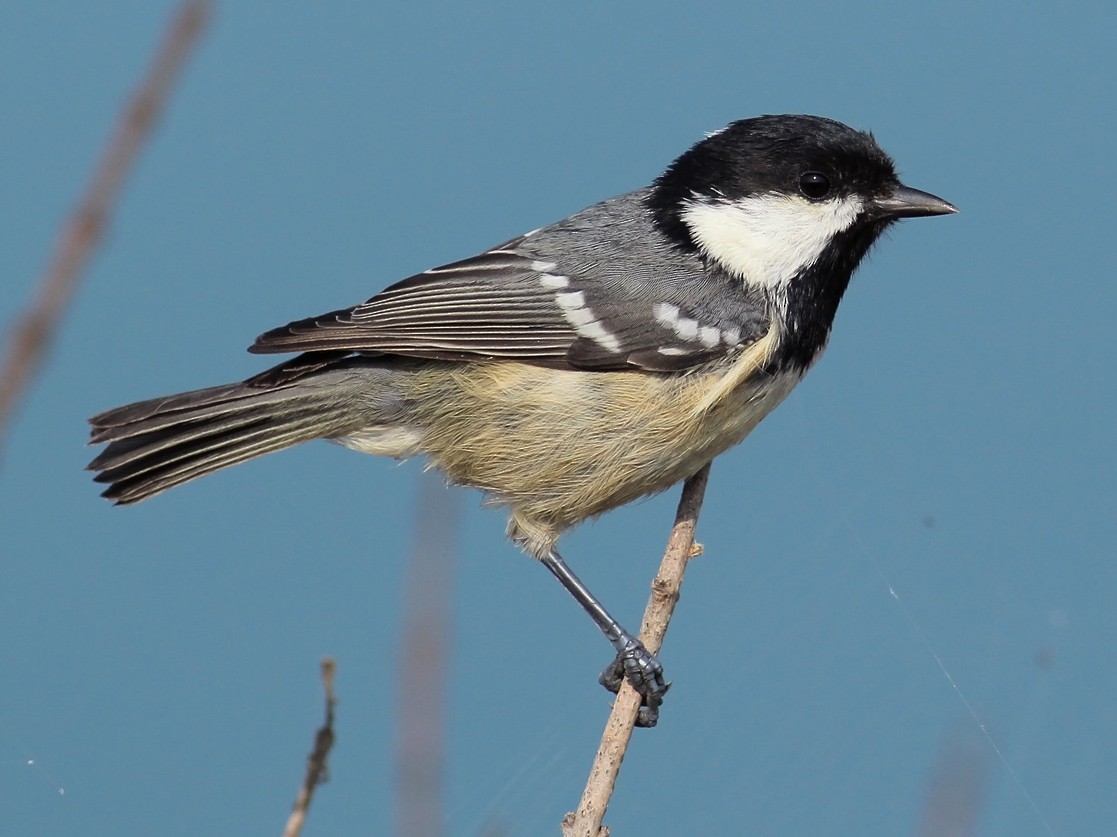
Individual differences related to changes in size, shape, and behavior that occur as an individual grows are called ontogenetic shifts. As you have experienced yourself, there are many changes that occur as an individual grows, and these changes can mean that different age classes have different specializations. Gustafsson (1988) found an ontogenetic shift in where coal tits (a species of bird) fed within a pine tree. Younger birds were more generalists but tended to feed on the outer sections of the tree, while adults foraged on the more profitable, central portion of the tree. He attributes this difference to dominance of adults over juveniles. Gustafsson also found that the larger individuals within each age class also tended to feed closer to the center of the tree. This within age class difference is attributed to a larger body size being better suited for feeding closer to the center of the tree, while smaller body sizes are better suited for hovering and foraging on the outside. Interestingly, this study occurred over multiple years, and Gustafsson documented several juvenile individuals that shifted foraging behavior when they became adults.
These sources of behavioral variation are important to account for because ultimately phenotypic variation can affect not only a population’s niche, but its population size, distribution, evolutionary potential, and vulnerability to environmental change (Wennersten & Forsman, 2012). And it’s important to determine which source(s) of variation are at play to inform best population management practices. Different behaviors between sexes versus age classes have different implications for the population, making it necessary to not only assess if there are differences but also to try and understand their drivers.
This behavioral variability relative to morphs is something that is of particular interest to me, and it is the focus of my first chapter. We’ve documented that the PCFG gray whales in our study region employ a variety of foraging tactics, and I want to know if there is specialization in tactic use and if we can find an underlying source of the variation. I can’t wait to share results with you in the next installment of this individual specialization journey. Stay tuned!
Did you enjoy this blog? Want to learn more about marine life, research, and conservation? Subscribe to our blog and get a weekly alert when we make a new post! Just add your name into the subscribe box below!
References
Bolnick, D. I., Amarasekare, P., Araújo, M. S., Bürger, R., Levine, J. M., Novak, M., Rudolf, V. H. W., Schreiber, S. J., Urban, M. C., & Vasseur, D. A. (2011). Why intraspecific trait variation matters in community ecology. Trends in Ecology & Evolution, 26(4), 183–192. https://doi.org/10.1016/j.tree.2011.01.009
Bolnick, D. I., Svanbäck, R., Fordyce, J. A., Yang, L. H., Davis, J. M., Hulsey, C. D., & Forister, M. L. (2003). The ecology of individuals: Incidence and implications of individual specialization. American Naturalist, 161(1), 1–28. https://doi.org/10.1086/343878
Cucherousset, J., Acou, A., Blanchet, S., Britton, J. R., Beaumont, W. R. C., & Gozlan, R. E. (2011). Fitness consequences of individual specialisation in resource use and trophic morphology in European eels. Oecologia, 167(1), 75–84. https://doi.org/10.1007/s00442-011-1974-4
Dall, S. R. X., Bell, A. M., Bolnick, D. I., & Ratnieks, F. L. W. (2012). An evolutionary ecology of individual differences. Ecology Letters, 15(10), 1189–1198. https://doi.org/10.1111/j.1461-0248.2012.01846.x
De Meyer, J., Belpaire, C., Boeckx, P., Bervoets, L., Covaci, A., Malarvannan, G., De Kegel, B., & Adriaens, D. (2018). Head shape disparity impacts pollutant accumulation in European eel. Environmental Pollution, 240, 378–386. https://doi.org/10.1016/j.envpol.2018.04.128
Gustafsson, L. (1988). Foraging behaviour of individual coal tits, Parus ater, in relation to their age, sex and morphology. Animal Behaviour, 36(3), 696–704. https://doi.org/10.1016/S0003-3472(88)80152-0
Kienle, S. S., Friedlaender, A. S., Crocker, D. E., Mehta, R. S., & Costa, D. P. (2022). Trade-offs between foraging reward and mortality risk drive sex-specific foraging strategies in sexually dimorphic northern elephant seals. Royal Society Open Science, 9(1), 210522. https://doi.org/10.1098/rsos.210522
Pianka, E. R. (1974). Niche Overlap and Diffuse Competition. 71(5), 2141–2145.
Sheppard, C. E., Inger, R., McDonald, R. A., Barker, S., Jackson, A. L., Thompson, F. J., Vitikainen, E. I. K., Cant, M. A., & Marshall, H. H. (2018). Intragroup competition predicts individual foraging specialisation in a group-living mammal. Ecology Letters, 21(5), 665–673. https://doi.org/10.1111/ele.12933
Wennersten, L., & Forsman, A. (2012). Population-level consequences of polymorphism, plasticity and randomized phenotype switching: A review of predictions. Biological Reviews, 87(3), 756–767. https://doi.org/10.1111/j.1469-185X.2012.00231.x
By Charles Nye, graduate student, OSU Department of Fisheries, Wildlife, & Conservation Sciences, Cetacean Conservation and Genomics Laboratory
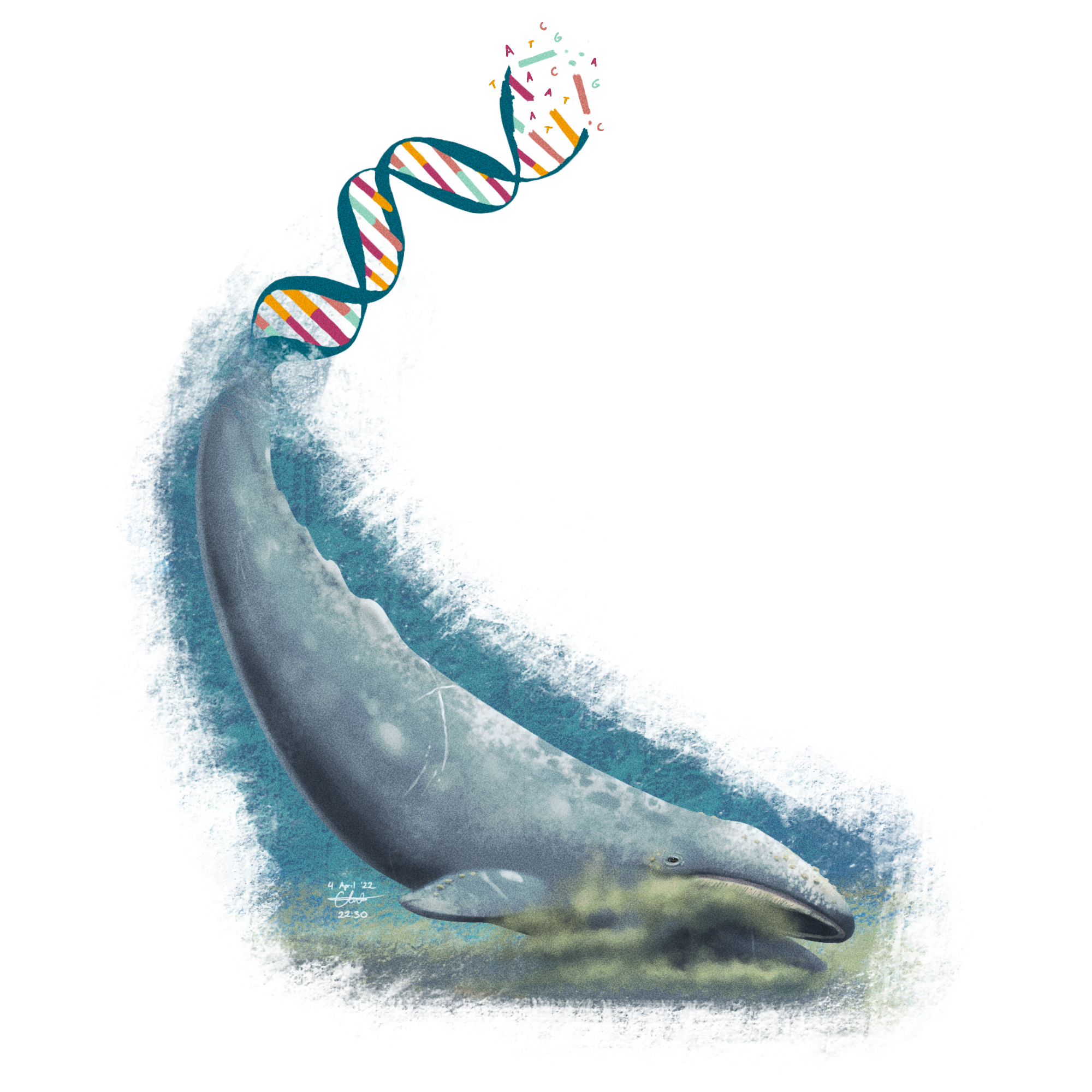
Figure 1: An illustration (by me) of a feeding gray whale whose caudal end transitions into a DNA double helix.
Let’s consider how much stuff organisms shed daily. If you walk down a hallway, you’ll leave a microscopic trail of skin cells, evaporated sweat, and even more material if you so happen to sneeze or cough (as we’ve all learned). The residency of these bits and pieces in a given environment is on the order of days, give or take (Collins et al. 2018). These days, we can extract, amplify, and sequence DNA from leftover organismal material in environments (environmental DNA; eDNA), stomach contents (dietary DNA, dDNA), and other sources (Sousa et al. 2019; Chavez et al. 2021).
You might be familiar with genetic barcoding, where scientists are able to use documented and annotated pieces of a genome to identify a piece of DNA down to a species. Think of these as genetic fingerprints from a crime scene where all (described) species on Earth are prime suspects. With advancements in computing technology, we can barcode many species at the same time—a process known as metabarcoding. In short, you can now do an ecosystem-wide biodiversity survey without even needing to see your species of interest (Ficetola et al. 2008; Chavez et al. 2021).
(Before you ask: yes, people have tried sampling Loch Ness and came up with not a single strand of plesiosaur DNA (University of Otago, 2019).)
I received my crash course on metabarcoding when I was employed at the Monterey Bay Aquarium Research Institute (MBARI), right before grad school. There, I was employed to help refine eDNA survey field and laboratory methods (in addition to some cool robot stuff). Here at OSU, I use metabarcoding to research whale ecology, detection, and even a little bit of forensics work. Cetacean species (or evidence thereof) I’ve worked on include North Atlantic right whales (Eubalaena glacialis), killer whales (Orcinus spp.), and gray whales (Eschrichtius robustus).
Long-time readers of the GEMM Lab Blog are probably quite knowledgeable about the summertime grays—the Pacific Coast Feeding Group (PCFG). All of us here at OSU’s Marine Mammal Institute (MMI) are keenly interested in understanding why these whales hang out in the Pacific Northwest during the summer months and what sets them apart from the rest of the Eastern North Pacific gray whale population. What interests me? Well, I want to double-check what they’re eating—genetically.
“What does my study species eat?” is a straightforward but underappreciated question. It’s also deceptively difficult to address. What if your species live somewhere remote or relatively inaccessible? You can imagine this is a common logistical issue for most research in marine sciences. How many observations do you need to make to account for seasonal or annual changes in prey availability? Do all individuals in your study population eat the same thing? I certainly like to mix and match my diet.
Gray whale foraging ecology has been studied comprehensively over the last several decades, including an in-depth stomach content evaluation by Mary Nerini in 1984 and GEMMer Lisa Hildebrand’s MSc research. PCFG whales seem to prefer shrimpy little creatures called mysids, along with Dungeness crab (Cancer magister) larvae, during their stay in the Pacific Northwest (PNW), most notably the mysid Neomysis rayii (Guerrero 1989; Hildebrand et al. 2021). Indeed, the average energetic values of common suspected prey species in PNW waters rival the caloric richness of Arctic amphipods (Hildebrand et al. 2021). However, despite our wealth of visual foraging observations, metabarcoding may add an additional layer of resolution. For example, the ocean sunfish (Mola mola) was believed to exclusively forage on gelatinous zooplankton, but a metabarcoding approach revealed a much higher diversity of prey items, including other bony fishes and arthropods (Sousa et al. 2016).
Given all this exposition, you may be wondering: “Charles—how do you intend on getting dDNA from gray whales? Are you going to cut them open?”
Figure 2: The battle station, a vacuum pump that I use to filter out all of the particulate matter from a gray whale dDNA sample. The filter is made of polycarbonate track etch material, which melts away in the DNA extraction process—quite handy, indeed!
No. I’m going to extract DNA from their poop.
Well, actually, I’ve been doing that for the last two years. My lab (Cetacean Conservation and Genomics Laboratory, CCGL) and GEMM Lab have been collaborating to make lemonade out of, er…whale poop. An archive of gray whale fecal samples (with ongoing collections every field season) originally collected for hormone analyses presented itself with new life—the genomics kind. In addition to community-level data, we are also able to recover informative DNA from the gray whales, including sex ID from “depositing” individuals, though the recovery rate isn’t perfect.
Because the GEMM Lab/MMI can non-invasively collect multiple samples from the same individuals over time, dDNA metabarcoding is a great way to repeatedly evaluate the diets of the PCFG, just shy of being at the right place at the right time with a GoPro or drone to witness a feeding event. While we can get stomach contents and even usable dDNA from a naturally deceased whale, those data may not be ideal. How representative a stranded whale is of the population is dependent on the cause of death; an emaciated or critically injured individual, for example, is a strong outlier.
Figure 3: Presence/absence of the top 10 most-common taxonomic Families observed in the PCFG gray whale dDNA dataset (n = 20, randomly selected). Filled-in dots indicate at least one genetic read associated with that Family, and empty dots indicate none. Note the prey taxa: mysids (Mysidae), krill (Euphausiidae), and olive snails (Olividae).
Here’s a snapshot of progress to date for this dDNA metabarcoding project. I pulled out twenty random samples from my much larger working dataset (n = 82) for illustrative purposes (and legibility). After some bioinformatic wizardry, we can use a presence/absence approach to get an empirical glimpse at what passes through a PCFG gray whale. While I am able to recover species-level information, using higher-level taxonomic rankings summarizes the dataset in a cleaner fashion (and also, not every identifiable sequence resolves to species).
The title of most commonly observed prey taxa belongs to our friends, the mysids (Mysidae). Surprisingly, crabs and amphipods are not as common in this dataset, instead losing to krill (Euphausiidae) and olive snails (Olividae). The latter has been found in association with gray whale foraging grounds but not documented in a prey study (Jenkinson 2001). We also get an appreciable amount of interference from non-prey taxa, most notably barnacles (Balanidae), with an honorable mention to hydrozoans (Clytiidae, Corynidae). While easy to dismiss as background environmental DNA, as gray whales do forage at the benthos, these taxa were physically present and identifiable in Nerini’s (1984) gray whale stomach content evaluation.
So—can we conclude that barnacles and hydrozoans are an important part of a gray whale’s diet, as much as mysids? From decades of previous observations, we might say…probably not. Gray whales are actively targeting patches of crabby, shrimpy zooplankton things, and even employ novel foraging strategies to do so (Newell & Cowles 2006; Torres et al. 2018). However, the sheer diversity of consumed species does present additional dimensionality to our understanding of gray whale ecology.
The whales are eating these ancillary organisms, whether they intend to or not, and this probably does influence population dynamics, recruitment, and succession in these nearshore benthic habitats. After all, the shallow pits that gray whales leave behind post-feeding provide a commensal trophic link with other predatory taxa, including seabirds and groundfish (Oliver & Slattery 1985). Perhaps the consumption of these collateral species affects gray whale energetics and reflects on their “performance”?
I hope to address all of this and more in some capacity with my published work and graduate chapters. I’m confident to declare that we can document diet composition of PCFG whales using dDNA metabarcoding, but what comes next is where one can get lost in the sea(weeds). How does the diet of individuals compare to one another? What about at differing time points? Age groups? How many calories are in a barnacle? No need to fret—this is where the fun begins!
References
Chavez F, Min M, Pitz K, Truelove N, Baker J, LaScala-Grunewald D, Blum M, Walz K,
Nye C, Djurhuus A, et al. 2021. Observing Life in the Sea Using Environmental
DNA Oceanog. 34(2):102–119. doi:10.5670/oceanog.2021.218.