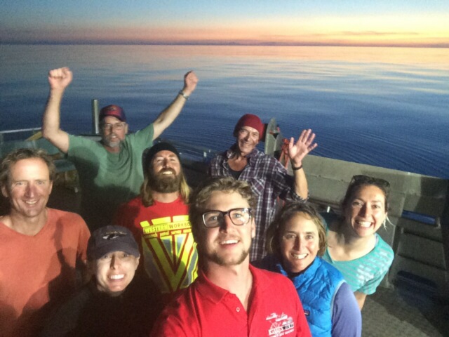
By Grace Hancock, Undergraduate Student at Kalamazoo College MI, GEMM Lab Intern (June 2020 to present)
It feels safe to say that everyone’s plans for the summer of 2020 went through a roller coaster of changes due to the pandemic. Instead of the summer research or travel plans that many undergraduate students, including myself, expected, many of us found ourselves at home, quarantining, and unsure of what to do with our time. Although it was unexpected, all that extra time brought me serendipitously to the virtual doorstep of the GEMM Lab. A few zoom calls and many, many emails later I am now lucky to be a part of the New Zealand Blue Whale photo-ID team. Under Leigh’s and Dawn’s guidance, I picked up the photo identification project where they had left it and am helping to advance this project to its next stage.
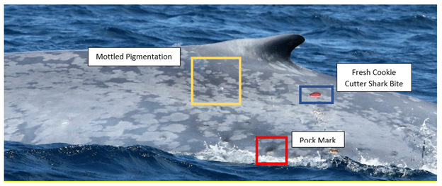
The skin of a blue whale is covered by distinct markings similar to a unique fingerprint. Thus, these whales can have a variety of markings that we use to identify them, including mottled pigmentation, pock marks (often caused by cookie cutter sharks), blisters, and even holes in the dorsal fins and flukes.
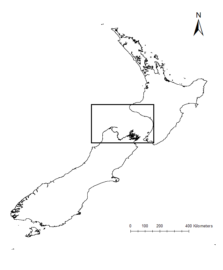
True blue blog fans may remember that in 2016 Dawn began the very difficult work of creating a photo ID catalog of all the blue whales that the GEMM Lab had encountered during field work in the South Taranaki Bight in New Zealand. Since that post, the catalog has grown and become an incredibly useful tool. When I came to the lab, I received a hard drive containing all the work Dawn had done to-date with the catalog, as well as two years of photos from various whale watching trips in the Hauraki Gulf of New Zealand. The goal of my internship was to integrate these photos into the GEMM catalog Dawn had created and, hopefully, identify some matches of whales between the two datasets. If there were any matches – and if I found no matches – we would gain information about whale movement patterns and abundance in New Zealand waters.
Before we could dive into this exciting matching work, there was lots of data organization to be done. Most of the photos I analyzed were provided by the Auckland Whale and Dolphin Safari (AWADS), an eco-tourism company that does regular whale watching trips in the Hauraki Gulf, off the North Island of New Zealand. The photos I worked with were taken by people with no connection to the lab and, because of this, were often filled with pictures of seals, birds, and whatever else caught the whale watcher’s eye. This dataset led to hours of sorting, renaming, and removing photos. Next, I evaluated each photo of a whale to determine photo-quality (focus, angle to the camera, lighting) and then I used the high-quality photos where markings are visible to begin the actual matching of the whales.

Blue whales are inarguably massive organisms. For this reason, it can be hard to know what part of the whale you’re looking at. To match the photos to the catalog, I found the clearest pictures that included the whale’s dorsal fin. For each whale I tried to find a photo from the left side, the right side, and (if possible) an image of its fluke. I could then compare these photos to the ones organized in the catalog developed by Dawn.
The results from my matching work are not complete yet, but there are a few interesting tidbits that I can share with our readers today. From the photos submitted by AWADS, I was able to identify twenty-two unique individual whales. We are in the process of matching these whales to the catalog and, once this is done, we will know how many of these twenty-two are whales we have seen before and how many are new individuals. One of the most exciting matches I made so far is of a whale known in our catalog as individual NZBW072. Part of what made this whale so exciting was the fact that it is the calf of NZBW031 who was spotted eight times from 2010-2017, in the Hauraki Gulf, off Kaikoura, and in the South Taranaki Bight. As it turns out, NZBW072 took after her mother and has been spotted a shocking nine times from 2010 to 2019, all in the Hauraki Gulf region. Many of the whales in our catalog have only been spotted once, so encountering two whales with this kind of sighting track record that also happen to be related is like hitting the jackpot.

Once I finish comparing and matching the rest of these photos, the catalog will be substantially more up-to-date. But that is not where the work stops. More photos of blue whales in New Zealand are frequently being captured, either by whale watchers in the Hauraki Gulf, fellow researchers on the water, keen workers on oil and gas rigs, or the GEMM Lab. Furthermore, the GEMM Lab contributes these catalog photos to the International Whaling Commission (IWC) Southern Hemisphere Blue Whale Catalog, which compiles all photos of blue whales in the Southern Ocean and enables interesting and critical conservation questions to be addressed, like “How many blue whales are there in the Southern Ocean?” Once I complete the matching of these 22 individuals, I will upload and submit them to this IWC collaborative database on behalf of the GEMM Lab. This contribution will expand the global knowledge of these whales and motivates me to continue this important photo ID work. I am so excited to be a part of this effort, through which I have learned important skills like the basics of science communication (through writing this blog post) and attention to detail (from working very closely with the photos I was matching). I know both of these skills, and everything else I have learned from this process, will help me greatly as I begin my career in the next few years. I can tell big things will come from this catalog and I will forever be grateful for the chance I have had to contribute to it.