By Natalie Chazal, PhD student, OSU Department of Fisheries, Wildlife, & Conservation Sciences, Geospatial Ecology of Marine Megafauna Lab
When most people think about monitoring the health of a 40-ton gray whale, they picture blubber thickness, dive patterns, or perhaps growth rates. But what if some of the most telling signs are found not in the whale’s bulk, but right on the surface–embedded in its skin, and even crawling across it?
As part of the GRANITE project, my research focuses on using a long-term photographic dataset (>347,000 photos from 10 years!) to evaluate epidermal indicators of stress and health in Pacific Coast Feeding Group (PCFG) gray whales (Eschrichtius robustus) foraging off the Oregon coast. My central questions ask:
- Can we use features visible on the skin like epidermal diseases, lesion severity, scarring from orcas, boats, and fishing gear, and potentially cyamid loads as biomarkers of physiological stress or nutritional status?
- How do these skin-based indicators correlate with environmental variables, prey availability, fecal hormones, and overall body condition?
By tracking these patterns across individuals and years, my goal is to understand how gray whales are responding to a changing ocean and whether their skin can tell us more about what’s under the surface.
What are cyamids?
Cyamids, more commonly known as “whale lice”, are small crustaceans that live exclusively on marine mammals. Despite their nickname, cyamids are not true lice—they’re actually amphipod ectoparasites, more closely related to beach hoppers than anything you’d find in your hair. For gray whales (Eschrichtius robustus), these tiny passengers are a constant presence throughout their lives.

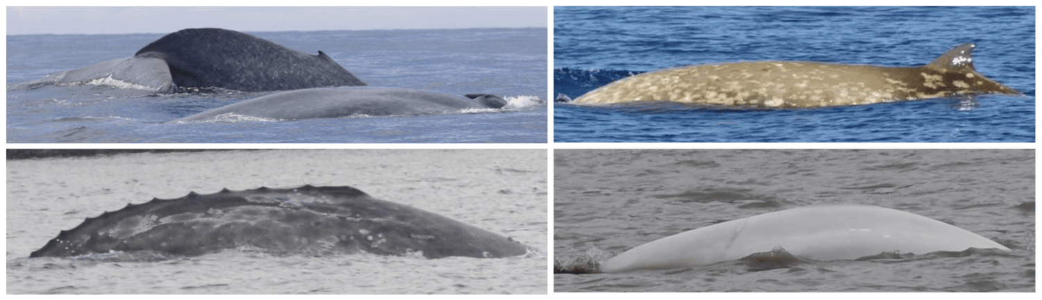
Each whale can host thousands of cyamids at a time, with individuals often clustering in specific areas of the body that provide physical refuge from the currents: around the blowhole, in the crevices of flukes, along the rostrum, genital slits, and especially around wounds or skin irregularities (Figure 1). Unlike barnacles, which attach directly to the skin and remain stationary while they feed on nutrients in the passing water, cyamids grasp onto the whale’s body using claw-like appendages, feeding on sloughed skin and bodily fluids. This relationship is generally not thought to be harmful to the whale, but high cyamid loads can be indicative of poor health, injury, or compromised immune function.
There are several species of cyamids, and many are host-specific—meaning they’ve evolved alongside particular whale species. In gray whales, the most common is Cyamus scammoni, which specializes on gray whales and is rarely found elsewhere. Other species found on gray whales include Cyamus kessleri, and the rarer Cyamus ceti. Cyamids are transmitted primarily from mother to calf, which helps explain their host fidelity, but horizontal transmission (between unrelated individuals) may also occur during close contact which can explain some rare occurrences of cyamids that are found outside of their general host species. In fact, Cyamus ceti was only found once on gray whales in 1861 but is generally thought to be specific to bowhead whales, giving us potential insight into interspecies interactions (bowhead and gray whales can spatially overlap on Arctic foraging grounds).

Because cyamids are permanent residents of the whale’s skin, they offer a unique window into both individual whale life histories and broader ecological trends. Their location, abundance, and distribution can potentially inform us about wound healing, residency duration in foraging areas, and even stress or health status—which makes them an unexpectedly valuable focal point in drone and photograph-based monitoring efforts like in the GRANITE project.
Cyamid Life History
Cyamids are obligate ectoparasites, meaning they spend their entire life on a whale and cannot survive independently in the open ocean. Unlike free-swimming crustaceans, cyamids are permanently attached to the skin or embedded within crevices of the whale’s body, often clinging to roughened areas, scars, embedded barnacles, or calloused skin where they can anchor themselves more securely.
They begin life as tiny juveniles, hatching from eggs carried in the brood pouch of a female cyamid. Rather than undergoing a larval phase in the water column like many marine invertebrates, cyamids develop directly into miniature versions of adults and remain on the whale from birth. This direct development is essential because there’s no safe habitat for a larval cyamid in the open ocean: the host whale is both nursery and home.
Most transmission occurs from mother to calf during the close physical contact of early life. Calves born in the warm lagoons of Baja California, Mexico where gray whales calve and nurse during the winter inherit their cyamid colonies during nursing, rubbing, and swimming alongside their mothers. These early colonizers will multiply as the calf grows and can remain with the whale for years, forming the basis of a persistent, host-specific population.
For Cyamus scammoni specifically (our gray whale specific cyamid), adults will breed in the summer just before the southbound migration. Females will have around 1,000 eggs in their brood pouch, although only about a 60% are fertilized (Leung, 1976). These eggs will hatch in the fall while the gray whales take on their southbound migration but they will stay in the safety of the brood pouch for around 2 to 3 months. The juveniles will be released in the winter, when gray whales arrive in the Baja lagoons where they will then find shelter within the crevices of their host gray whale. Juveniles reach maturity during the northbound migration and will be a full-grown brood upon arrival to summer grounds. While the cycle takes about 8 months to complete, there are juveniles found along the gray whales year-round, leading us to believe that there is likely overlap between broods. For our less abundant Cyamus kessleri, the life cycle is very similar, but the juveniles reach maturity before the gray whales northbound migration to summer feeding grounds. Also, there are around 300 eggs in the Cyamus kessleri brood pouches that have a higher rate of fertilization (75-80%) than Cyamus scammoni (60%) (Leung, 1976)
In short, the life of a cyamid is fully bound to the life of a whale. Every migration, dive, foraging event, and scar the whale experiences becomes part of the cyamid’s environment. By studying them, we gain another lens through which to interpret the health, behavior, and ecology of gray whales on the Oregon Coast.
Uses in Cetacean Health Assessments
As we’ve established, cyamids have unique life histories as ectoparasites and may be valuable indicators in cetacean health assessments across multiple whale species. Because they often congregate around wounds, lesions, and areas of poor skin integrity, their presence and distribution can reveal important clues about a whale’s physical condition, injury history, and immune response. However, studies that have made these connections have variable results.
In species like North Atlantic right whales (Pettis et al. 2004, Pirotta et al. 2023), harbor porpoises (Lehnert et al. 2021), and gray whales (Raverty et al. 2024), researchers have used visual surveys and photographic analysis to quantify cyamid loads in living, stranded, and hunted whales. Researchers can score cyamid presence by identifying attachment sites (e.g. blowhole, scar, dorsal ridge) and estimating the relative coverage by using standardized reference images to maintain consistency. In these studies, whales with heavy cyamid coverage, especially in sensitive regions like the blowhole, mouthline, and genital area, often show signs of poor health or stress, such as emaciation, scarring from entanglement, or chronic skin conditions. Cyamid coverage is sometimes used alongside body condition indices and lesion scoring to build a more complete health profile (Pirotta et al. 2023). There are also studies that show no connections, or even positive connections between body condition and cyamid coverage (Von Duyke et al. 2016).
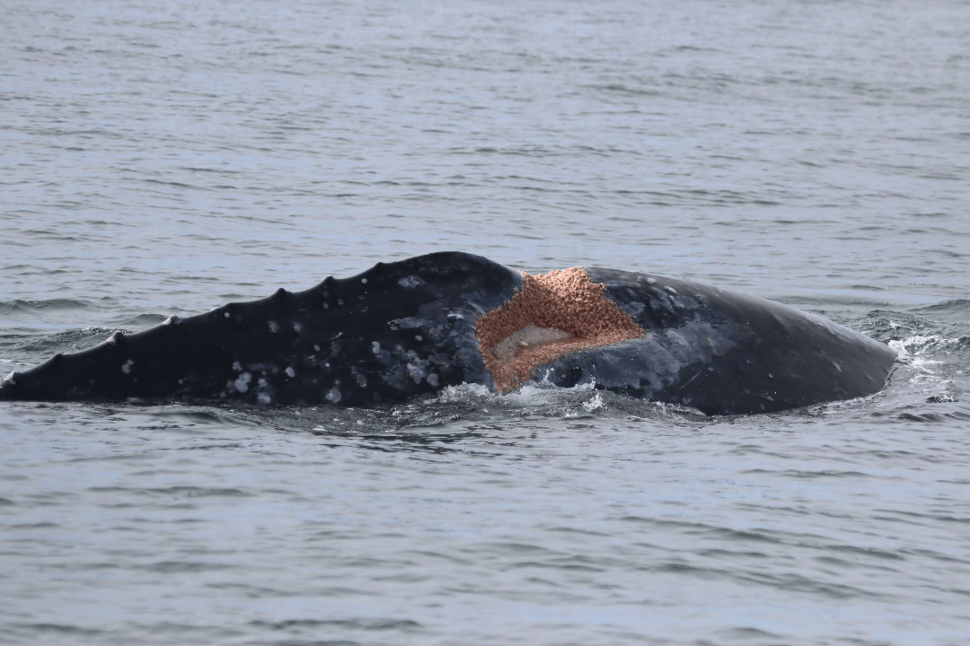
While cyamids are often associated with injured, inflamed, or otherwise damaged skin, there is no evidence that points towards cyamids directly damaging the skin themselves. However, more work needs to be done to assess their role in the healing processes. Additionally, it’s been noted that more work is needed on the role of cyamids and disease spread (Overstreet et al. 2009). For the PCFG, there is an iconic whale we call “Scarlett” (also known as “Scarback”) who has a large scar on the right side of her back that is highly identifiable due to the orange swarm of cyamids that are constantly surrounding the edges of the wound. She has managed to survive and thrive, producing many calves over the years, but questions remain: How are the cyamids affecting the healing process? Are they increasing or decreasing the risk of infection? How does the frequency of large injuries like this on whales contribute to the cyamid population over evolutionary time?
Because whales are complex, highly mobile, long-lived creatures with a constant population of cyamid hitchhikers their skin condition is likely representative of specific to life history, phylogeography, and demographic traits of individuals. While we know that cyamids generally eat sloughed or damaged skin on the whale, what this behavior and symbiosis means for each whale’s individual physiology can be highly complex. Through our high-resolution drone and lateral imagery of the same individuals over time paired with other data sources, such as body condition and prey availability, cyamid scores can offer key insights into how environmental stressors and foraging success affect individual and population-level whale health.
These tiny crustaceans, clinging to the folds and scars of their hosts, might seem like background noise in a study focused on body condition or foraging ecology—but they’re far from incidental. In my research, I’ve come to see cyamids as part of the bigger story: silent indicators of stress, recovery, movement, and resilience. By pairing imagery of PCFG gray whale skin with data on prey availability and environmental conditions, I’m working to understand how foraging success and anthropogenic stressors (such as vessel traffic and entanglements) manifest not just in a whale’s body condition, but in the skin itself. The presence, distribution, and density of cyamids may offer yet another layer of insight into how gray whales are coping with changing ocean conditions. It’s a reminder that even the smallest details, like a patch of whale lice, can help us ask bigger questions about the health, resilience, and future of these cetaceans.
References
Callahan, C.M., n.d. MOLECULAR SYSTEMATICS AND POPULATION GENETICS OF WHALE LICE (AMPHIPODA: CYAMIDAE) LIVING ON GRAY WHALE ISLANDS.
Lehnert, K., IJsseldijk, L.L., Uy, M.L., Boyi, J.O., van Schalkwijk, L., Tollenaar, E.A.P., Gröne, A., Wohlsein, P., Siebert, U., 2021. Whale lice (Isocyamus deltobranchium & Isocyamus delphinii; Cyamidae) prevalence in odontocetes off the German and Dutch coasts – morphological and molecular characterization and health implications. International Journal for Parasitology: Parasites and Wildlife 15, 22–30. https://doi.org/10.1016/j.ijppaw.2021.02.015
Leung, Y., 1976. Life cycle of cyamus scammoni (amphipoda: cyamidae), ectoparasite of gray whale, with a remark on the associated species. Scientific Reports of the Whales Research Institute 28, 153–160.
Overstreet, R.M., Jovonovich, J., Ma, H., 2009. Parasitic crustaceans as vectors of viruses, with an emphasis on three penaeid viruses. Integrative and Comparative Biology 49, 127–141. https://doi.org/10.1093/icb/icp033
Pettis, H.M., Rolland, R.M., Hamilton, P.K., Brault, S., Knowlton, A.R., Kraus, S.D., 2004. Visual health assessment of North Atlantic right whales (Eubalaena glacialis) using photographs. Can. J. Zool. 82, 8–19. https://doi.org/10.1139/z03-207
Pirotta, E., Schick, R.S., Hamilton, P.K., Harris, C.M., Hewitt, J., Knowlton, A.R., Kraus, S.D., Meyer-Gutbrod, E., Moore, M.J., Pettis, H.M., Photopoulou, T., Rolland, R.M., Tyack, P.L., Thomas, L., 2023. Estimating the effects of stressors on the health, survival and reproduction of a critically endangered, long-lived species. Oikos 2023, e09801. https://doi.org/10.1111/oik.09801
Raverty, S., Duignan, P., Greig, D., Huggins, J.L., Huntington, K.B., Garner, M., Calambokidis, J., Cottrell, P., Danil, K., D’Alessandro, D., Duffield, D., Flannery, M., Gulland, F.M., Halaska, B., Lambourn, D.M., Lehnhart, T., Urbán R., J., Rowles, T., Rice, J., Savage, K., Wilkinson, K., Greenman, J., Viezbicke, J., Cottrell, B., Goley, P.D., Martinez, M., Fauquier, D., 2024. Gray whale (Eschrichtius robustus) post-mortem findings from December 2018 through 2021 during the Unusual Mortality Event in the Eastern North Pacific. PLoS One 19, e0295861. https://doi.org/10.1371/journal.pone.0295861
Stimmelmayr, R., Gulland, F.M.D., 2020. Gray Whale (Eschrichtius robustus) Health and Disease: Review and Future Directions. Front. Mar. Sci. 7. https://doi.org/10.3389/fmars.2020.588820
Takeda, M., Ogino, M., n.d. Record of a Whale Louse, Cyamus scammoni Dall (Crustacea: Amphipoda: Cyamidae), from the Gray Whale Strayed into Tokyo Bay, the Pacific Coast of Japan.
Von Duyke, A.L., Stimmelmayr, R., Sheffield, G., Sformo, T., Suydam, R., Givens, G.H., George, J.C., 2016. Prevalence and Abundance of Cyamid “Whale Lice” (Cyamus ceti) on Subsistence Harvested Bowhead Whales (Balaena mysticetus). Arctic 69, 331–340.
Würsig, B., Thewissen, J.G.M., Kovacs, K.M., 2017. Encyclopedia of Marine Mammals. Elsevier Science & Technology, Chantilly, UNITED STATES.