By Morgan O’Rourke-Liggett, Master’s Student, Oregon State University, Department of Fisheries, Wildlife, and Conservation Sciences, Geospatial Ecology of Marine Megafauna Lab
Avid readers of the GEMM Lab blog and other scientists are familiar with the incredible amounts of data collected in the field and the informative figures displayed in our publications and posters. Some of the more time-consuming and tedious work hardly gets talked about because it’s the in-between stage of science and other fields. For this blog, I am highlighting some of the behind-the-scenes work that is the subject of my capstone project within the GRANITE project.
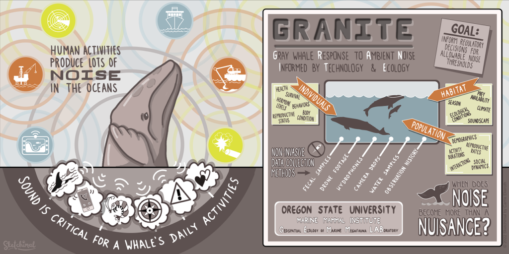
For those unfamiliar with the GRANITE project, this multifaceted and non-invasive research project evaluates how gray whales respond to chronic ambient and acute noise to inform regulatory decisions on noise thresholds (Figure 1). This project generates considerable data, often stored in separate Excel files. While this doesn’t immediately cause an issue, ongoing research projects like GRANITE and other long-term monitoring programs often need to refer to this data. Still, when scattered into separate long Excel files, it can make certain forms of analysis difficult and time-consuming. It requires considerable attention to detail, persistence, and acceptance of monotony. Today’s blog will dive into the not-so-glamorous side of science…data management and standardization!

Of the plethora of data collected from the GRANITE project, I work with the GPS trackline data from the R/V Ruby, environmental data recorded on the boat, gray whale sightings data, and survey summaries for each field day. These come to me as individual yearly spreadsheets, ranging from thirty entries to several thousand. The first goal with this data is to create a standardized survey effort conditions table. The second goal is to determine the survey distance from the trackline, using the visibility for each segment, and calculate the actual area surveyed for the segment and day. This blog doesn’t go into how the area is calculated. Still, all these steps are the foundation for finding that information so the survey area can be calculated.
The first step requires a quick run-through of the sighting data to ensure all dates are within the designated survey area by examining the sighting code. After the date is a three-letter code representing a different starting location for the survey, such as npo for Newport and dep for Depoe Bay. If any code doesn’t match the designated codes for the survey extent, those are hidden, so they are not used in the new table. From there, filling in the table begins (Figure 2).

Segments for each survey day were determined based on when the trackline data changed from transit to the sighting code (i.e., 190829_1 for August 29th, 2019, sighting 1). Transit indicated the research vessel was traveling along the coast, and crew members were surveying the area for whales. Each survey day’s GPS trackline and segment information were copied and saved into separate Excel workbook files. A specific R code would convert those files into NAD 1983 UTM Zone 10N northing and easting coordinates.
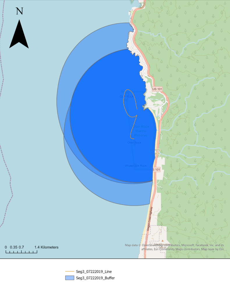
Those segments are uploaded into an ArcGIS database and mapped using the same UTM projection. The northing and easting points are imported into ArcGIS Pro as XY tables. Using various geoprocessing and editing tools, each segmented trackline for the day is created, and each line is split wherever there was trackline overlap or U shape in the trackline that causes the observation area to overlap. This splitting ensures the visibility buffer accounts for the overlap (Figure 3).

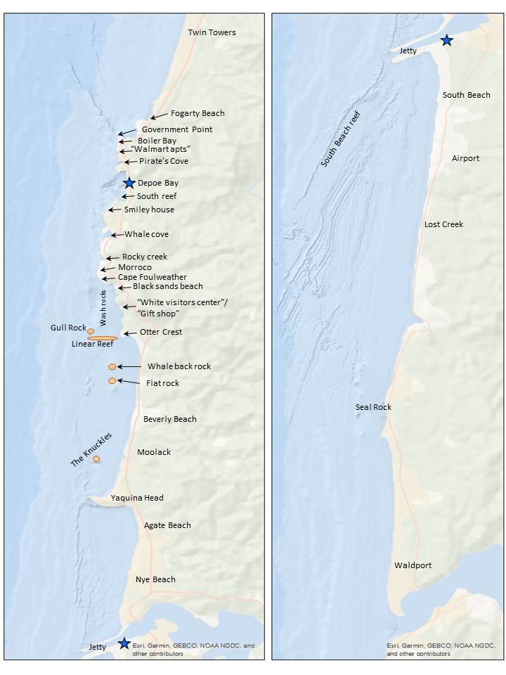
Once the segment lines are created in ArcGIS, the survey area map (Figure 4) is used alongside the ArcGIS display to determine the start and end locations. An essential part of the standardization process is using the annotated locations in Figure 4 instead of the names on the basemap for the location start and endpoints. This consistency with the survey area map is both for tracking the locations through time and for the crew on the research vessel to recognize the locations. The step assists with interpreting the survey notes for conditions at the different segments. The time starts and ends, and the latitude and longitude start and end are taken from the trackline data.

The sighting data includes the number of whales sighted, Beaufort Sea State, and swell height for the locations where whales were spotted. The environmental data from the sighting data is used as a guide when filling in the rest of the values along the trackline. When data, such as wind speed, swell height, or survey condition, is not explicitly given, matrices have been developed in collaboration with Dr. Leigh Torres to fill in the gaps in the data. These matrices and protocols for filling in the final conditions log are important tools for standardizing the environmental and condition data.
The final product for the survey conditions table is the output of all the code and matrices (Figure 5). The creation of this table will allow for accurate calculation of survey effort on each day, month, and year of the GRANITE project. This effort data is critical to evaluate trends in whale distribution, habitat use, and exposure to disturbances or threats.

The process of completing the table can be a very monotonous task, and there are several chances for the data to get misplaced or missed entirely. Attention to detail is a critical aspect of this project. Standardizing the GRANITE data is essential because it allows for consistency over the years and across platforms. In describing this aspect of my project, I mentioned three different computer programs using the same data. This behind-the-scenes work of creating and maintaining data standardization is critical for all projects, especially long-term research such as the GRANITE project.
Did you enjoy this blog? Want to learn more about marine life, research, and conservation? Subscribe to our blog and get a weekly message when we post a new blog. Just add your name and email into the subscribe box below.
