By Anthony Howe, Astoria High School graduate 2019, GEMM Lab summer intern
Murphy’s Law says that “things will go wrong in any given situation if you give them a chance”. This statement certainly applies to research where you never really know what is going to happen when performing fieldwork. You can only try to be prepared for all of the situations. When I arrived at the Oregon State University (OSU) Field Station in Port Orford, I had no idea that it would harbor some of the best educational experiences I have ever had. I had no idea what a theodolite was, nor did I know how to kayak in the ocean, but I learned fast. When we first started being trained on using a theodolite and the program that processes the data, Pythagoras, we had some problems. The theodolite would not stay level, but just as we were learning how to work the theodolite, we also learned how to work as a team. When we finally managed to level the theodolite, which did take a few days, I began to realize the hard work of doing fieldwork. You can be prepared but there will always be something that goes wrong, and that’s okay. I have learned that mistakes happen and cannot be dwelled on. Only learned from. No one is perfect.
Fig 1. Me holding two zooplankton samples after collecting them on the kayak. Source: L. Hildebrand.
Just two days ago I was on our tandem research kayak with Mia Arvizu, the OSU Marine Studies Initiative (MSI) undergraduate intern. When we go out on the kayak, we paddle around our study area and go to GPS-marked “stations” to collect prey samples of zooplankton, test for water visibility using a Secchi disk, and send a GoPro underwater to have a better understanding of what is going on under the surface. While sampling at Station 15 in Mill Rocks I lowered the GoPro into the water using a downrigger. When the GoPro reached the bottom, I began to pull it up, only to realize it had gotten snagged in a crevice. I gave the line to which the GoPro is attached some slack and began to give Mia instructions to move to different spots to try and retrieve the GoPro out of this tight crevice. Unfortunately, I did not realize all of the lines had wrapped themselves underneath the downrigger and as soon as a swell came up, the line broke. My eyes widened as I realized what had just happened. Thankfully, I managed to grasp the last of the remaining line left connected to the GoPro and pulled it back into the kayak using my hand wrapped in a towel since the line is thin and can cut into your hands easily. Only then did I realize that neither Mia nor I had packed a knife in the event we needed to cut a line. We sat and pondered ideas of how to cut the last of the line so that I could reattach the GoPro to the downrigger. Mia came up with the idea to use a barnacle or a mussel, and it worked perfectly. We were proud of ourselves for being resourceful and using nature to our advantage. But as soon as I finished using the mussel to cut the line, Lisa’s voice came over the VHF radio that we always carry with us in the kayak that there were scissors in the First Aid Kit that is stowed in the dry hatch of the kayak. Mia and I looked at each other and could only laugh. The kayak team can be rough at times but it’s made up by the fact that we get beautiful prey samples and stunning GoPro videos of what is below the water.
Fig 2. Mia and myself paddling the kayak across “The Passage”, the approximately 1 km stretch between Mill Rocks and Tichenor Cove, our two study sites. Red Fish Rocks, which is Oregon’s first Marine Reserve, can be seen in the background. Source: L. Hildebrand.
After all of the kayak sampling is done we organize and store our gear, and then go to the lab. In the lab, one person will clean all tools and devices touched by saltwater while the other sieves all of our zooplankton samples. Each sample is individually sieved and then placed in a sample jar with its station name on it and placed into the freezer. We put them in the freezer to increase the longevity of the samples, as well as euthanizing all zooplankton so that they are easier to identify under a dissection scope. After all of that is done we take a 45-minute break before taking over the cliff team job so they can have a lunch break, as well as a rest from staring at the glare of the water all day searching for whales.
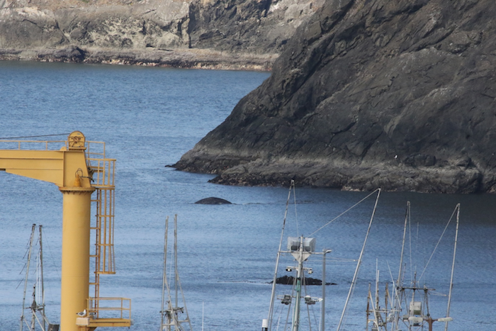
The cliff team generally consists of two people. One person will be on the theodolite, and the other will be on the laptop. The idea is that the theodolite uses the Pythagorean Theorem to get the exact coordinates of the whale we are spotting. This allows us to track exactly where the whales are going, what they are doing, how they’re doing it, and the fashion in which they’re doing it. The fixed points will fall on a plotted map on the laptop. The other job of the person on the laptop is to take pictures when possible so we can identify the whales. For instance, there is a whale named Buttons that has been recorded during past summers in Port Orford. By using the photos we take of a whale, combined with previous data about the whale named Buttons, we can cross-reference the body color and patterns of the whale to be able to re-identify Buttons. We now know that we have seen Buttons for 4 consecutive days feeding in our study area. The camera also acts as a tool to take pictures of whales not just for identity but for rare activity. Today while on the cliff Mia and I spotted a whale in Tichenor Cove (one of our sampling sites) that breached four times! These experiences are rare and beautiful. You never think about how big a whale truly is until you see it almost completely leap out of the water – it is beautiful.
Fig 3. The post-breach splash created by Buttons. Unfortunately we weren’t able to get a good photo from the cliff because we were too stunned by the fact that we were seeing this rare behavior. Source: GEMM Lab.
I’m sure more mistakes will be made but that’s okay. I have many more experiences to witness, and many more memories to make from this internship, as well as challenges. I couldn’t be more than happy with the team I have to share all of these learning experiences and hardships with.
By Lisa Hildebrand, MSc student, OSU Department of Fisheries and Wildlife, Geospatial Ecology of Marine Megafauna Lab
It seems unfathomable to me that one year and two months ago I had never used a theodolite before, never been in an ocean kayak before, never identified zooplankton before, never seen a Time-Depth-Recorder (TDR) before. Now, one year later, it seems like all of those tools, techniques and things are just a couple of old friends with which I am being reunited with again. My second field season as the project team lead of the gray whale foraging ecology project in Port Orford (PO) is slowly getting underway and so many of the lessons I learned from my first field season last year have already helped me tremendously this year. I know how to interpret weather forecasts and determine whether it will be a kayak-appropriate day. I know how to figure out the quirks of Pythagoras, the program we use to interface with our theodolite which helps us track whales from our cliff site. I know how to keep track of a budget and feed a team of hungry researchers after a long day of work. Knowing all of these things ahead of this year’s field season have made me feel a little more prepared and at ease with the training of my team and the work to be done. Nevertheless, there are always new curveballs to be thrown my way and while they can often be frustrating, I enjoy the challenges that being a team leader has to offer as it allows me to continue to grow as a field research scientist.
Figure 1. Crew Cinco tracks a whale in Tichenor Cove. Source: L Hildebrand.
2019 marks the fifth year that this project has been taking place in PO. Back in the summer of 2015, former GEMM Lab Master’s student Florence Sullivan started this project together with Leigh. That year the research focused more on investigating vessel disturbance to gray whales by comparing sites of heavy (Boiler Bay) to low boat traffic (Port Orford). The effort found that there were significant differences in gray whale activity budgets between the heavy and low boat traffic conditions (Sullivan & Torres 2018). The following year, the focus of the research switched to being more on the foraging ecology side of things and the project was based solely out of Port Orford, as it continues to be to this day. Being in our fifth year means that we are starting to build a humbly-sized database of sightings across multiple years allowing me to investigate potential individual specialization of the whales that we document. Similarly, multiple years of prey sampling is starting to reveal temporal and spatial trends of prey community assemblages.
Figure 2. Buttons (pictured above) is one of the stars of the Port Orford gray whale foraging ecology project as he has been seen every year since 2016. Crew Cinco has already seen him three times since the start of August. Source: L Hildebrand.
It has become a tradition to come up with a name for the field team that spends 6 weeks at the Oregon State University (OSU) Port Orford Field Station to collect the data for the project. It started with Team Ro“buff”stus in 2015, which I believe carried through until 2017. This is understandable since it’s such a clever name. It’s a play on the species name for gray whales, robustus, but the word “Buff” has been substituted in the center. Buffs are pieces of cloth sewn into a cylindrical shape, often with fun patterns or colors, that can be used as face masks, headbands, and scarves, which come in very handy when your face is exposed to the elements. Doing this project, we can be confronted by wind, sun, fog and sea water all in one day, so Buffs have definitely served the team members very well over the years. Last year, as the project’s torch was passed from Florence to myself, I felt a new team name was apt, and so last year’s team decided our name would be Team Whale Storm. I believe it was because we said we would take the whale world by storm with our insanely good theodolite tracking and kayak sampling skills. With a new year and new team upon us, a new team name was in order. As the title of this blog post indicates, this year the team is called Crew Cinco. The reason behind this name is that we are the fifth team to carry out this field work. Since the gray whales breed in the lagoons of Baja California, Mexico, I like to think that their native language is Spanish. Hence, we have decided that instead of being Crew Five, we are Crew Cinco, as cinco is the Spanish word for five (besides, alliteration makes for a much better team name).
Now that you are up to speed on the history of the PO gray whale project, let me tell you a little about who is part of Crew Cinco and what we have been up to already.
This year’s Marine Studies Initiative OSU undergraduate intern is Mia Arvizu. Mia has just finished her sophomore year at OSU and majors in Environmental Science. Besides being my co-captain this year in the field, Mia is also undertaking an independent research project which focuses on the relationship between sea urchin abundance, kelp health and gray whale foraging. She will tell you all about this project in a few weeks when she takes over the GEMM lab blog. Aside from her interest in ecology and the way science can be used to help local communities in a changing environment, Mia is a dancer, having performed in several dances in OSU’s annual luau this year, and she is currently teaching herself Spanish and Hawaiian.
Both of our high school interns this year are from Astoria. Anthony Howe has just graduated from Astoria High School and will be starting at Clatsop Community College in the fall. His plan is to transfer to OSU and to pursue his interest in marine biology. Anthony, like myself, was born in Germany and lived there until he was six, which means that he is able to speak fluent German. He also introduced the team to the wonders of the Instant Pot, which has made cooking for a team of four hungry scientists much simpler.
Donovan Burns is our other high school intern. He will be going into his junior year in the fall. Donovan never ceases to amaze us with the seemingly endless amounts of general knowledge he has, often sharing facts about Astoria’s history to Asimov’s Laws of Robotics to pickling vegetables, specifically carrots, with us during dinner or while scanning for whales on the cliff site. He also named the first whale we saw here this season – Speckles.
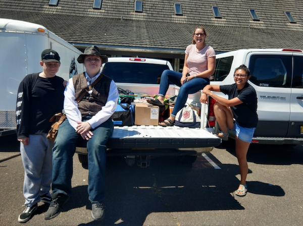
Figure 3. Crew Cinco, from left to right: Anthony Howe, Donovan Burns, Lisa Hildebrand and Mia Arvizu. Source: L Torres.
Crew Cinco has already been in PO for two weeks now. After having a full team meeting with Leigh in Newport and a GEMM lab summer pizza party, we headed south to begin our 6-week field season. It’s hard to believe that the two training weeks are already over. The team worked hard to figure out the subtleties of the theodolite, observe different gray whales and start to understand their dive and foraging patterns, undertake a kayak paddle & safety course, as well as CPR and First Aid training, learn about data processing and management, and how to use a variety of gizmos to aid us in data collection. But it hasn’t all been work. We enjoyed a day in the Californian Redwoods on one of our day’s off and picked blueberries at the Twin Creek Ranch, stocking our freezer with several bags of juicy berries. We have played ‘Sorry!’ perhaps one too many times already (we are in desperate need of some more boardgames if anyone wants to send some our way to the field station!), and enjoyed many walks and runs on beautiful Battle Rock Beach.
Crew Cinco in awe of the Redwoods
Crew Cinco’s blueberry harvest
Crew Cinco after their kayak paddle & safety course South Coast Tours
The next four weeks will not be easy – very early mornings, lots of paddling and squinting into the sun, followed by several hours in the lab processing samples and backing up data. But the next four weeks will also be extremely rewarding – learning lots of new skills that will be valuable beyond this 6-week period, revealing ecological trends and relationships, and ultimately (the true reason for why Mia, Anthony, Donovan and myself are more than happy to put in 6 weeks-worth of hard work), the chance to see whales every day up close and personal. Follow Crew Cinco’s journey over the next few weeks as my interns will be posting to the blog for the next three weeks!
References
Sullivan, F.A., & Torres L.G. Assessment of vessel disturbance to gray whales to inform sustainable ecotourism. Journal of Wildlife Management, 2018. 82: 896-905.
I graduated in March 2017 from the GEMM lab at Oregon State, with a Master’s of Science in Wildlife Management. Graduate school was finally over! No more constant coffee refills, popcorn dinners and overnight library stays; I had submitted my final thesis and I was done! Graduate school was no walk in the park for me, and finishing a master’s or a doctorate degree for anyone is no easy feat! It takes years of hard work, commitment, long hours, and a dedication to learning. I remember feeling both excited and a bit disoriented to be done with this phase of much stress and growth. After submitting my thesis, I took a much-needed month off to unknot the muscles in my back and get myself reacquainted with sunlight. The breath of fresh air was exactly what I needed to recover, but it took no time at all for a new type of challenge to emerge: the arduous task of finding a job.
I did what most job seekers do, I sat behind my computer
applying for opportunities, hit as many roles as I could, and hoped for the
best. Days turned into weeks and weeks turned into months. I was getting
desperate, I resorted to applying for a whole spectrum of roles – consulting,
project management, administration, youth team leader – hoping that something
would land. Soon enough, almost 3 months had passed and I was still in the same
spot as before. I was ready to throw in the towel.
In theory, landing a job after graduation sounds like it should be technically easy because more education should mean you are more qualified for the job, but anyone who has been out of grad school for more than an hour can tell you that landing a job after graduate school can be a long and frustrating process. I did not enter this field and its job prospects blindly – that is, I had a working idea of what type of research career I wanted when I completed my education and how much education I would need to get there. I was aware that navigating the job market in a competitive field could be tricky and time-consuming, especially as a green-job seeker. I knew it would be an added difficulty to land a position near the ocean but also close enough to family (I’m from the Midwest). Or at least, I thought I knew how hard it would be to secure a job. The process turned out to be much harder. Mental preparation alone was not enough and months and months of rejection and feeling stuck within the hamster wheel of the job search cycle was becoming my normal.
So, when I was stuck in the depths of a seemingly fruitless
job search, and trying as hard as I possibly could, it was hard for me to do
anything but roll my eyes, sigh, and give up. But I had to find a way to work
through an apparently endless string of rejection by figuring out some way to
accept, address and navigate my emotions. I needed to take charge of my own
personal development. I started reflecting on what areas of my work on my
master’s thesis that I found most difficult and wanted to improve, and would be
an important component of the job I
wanted. Identifying my own “knowledge gaps” led me to seek out courses,
workshops, job-shadowing and online courses that could fill those holes.
The first thing at the top of my list was to be more
efficient at coding.
Every job description that made me excited to apply had some description of a
coding program: R, Python, MATLAB. I was
lucky enough to attend courses and workshops during my time at the GEMM lab
that provided me much of the code I would need to create my habitat models with
minimal tweaking. On top of that I was surrounded by supervisors and a lab full
of coding geniuses that had an almost, if not completely, open door policy.
When I was stuck and a deadline was quickly approaching, it was great to have
an army of people to help me get through my obstacles. However, I knew if I
wanted to be successful, I needed to become like them: experts and not a
beginner. I purchased a subscription to DataCamp, and started
searching out courses that could help keep my skills fresh and learn new
things. I was over the moon to discover the course “Where are the Fishes?”.
It checked all my boxes: geospatial analysis, R, marine related, acoustics….
perfect. Within this course, there were plenty of DataCamp prerequisites, like
working with data in the tidyverse and working with dates and times in R, so I
had plenty to keep me busy.
I also started looking for in-person, hands-on courses I could enroll in. Since the majority of my marine experience took place on the west coast but I was searching for jobs on the east coast, I enrolled in the Marine Mammal and Sea Turtle Observer Certification Course for the US Atlantic and Gulf of Mexico Oceans in order to learn a little more about identifying species I did not commonly see in nearshore, northern Pacific waters. In this course, I learned about regulations surrounding protected species monitoring, proper camera settings for photographing marine life, and gained the certification needed to work as an observer during seismic surveys for Bureau of Ocean Energy Management (BOEM) and Bureau of Safety and Environmental Enforcement (BSEE) in coordination with the National Marine Fisheries Service. Most of these topics were familiar to me, other than identifying new species, but it was nice to have the refresher and the renewed certification. Heads up this course is coming to Newport in October and I highly recommend it! During this observer course in Charleston, I was able to network with others in the field taking the course, the Charleston aquarium, and the South Carolina DNR. By introducing myself and providing a little bit of my background, I was invited by the South Carolina DNR to watch a satellite tag and release of a sea turtle that the aquarium had been rehabilitating. From the sea turtle release I learned of the International Sea Turtle Symposium that would take place in February in Myrtle Beach, North Carolina and was invited to attend and network by one of the conference chairs, which lead me to my current position. See below…
Releasing of a satellite-tagged Kemp’s Ridley Sea Turtle off Foley Beach, South Carolina
Downtown Charleston
I tried everything I could to keep myself attached to the field. I attended the Biannual Marine Mammal Conference, enrolled in a bioacoustics short course, watched webinars every Friday, read recent journal articles, looked for voluntary work. I even dropped in on offices like NOAA or Universities of towns I was driving through or visiting to see what they were researching, and if they were looking for researchers. Continuous learning and developing took a lot of time, money, and energy but being conscientious about my personal development kept me motivated and engaged. Graduate school prepared me for all of this. My GEMM lab experience taught me to be open to learning, to be flexible and adaptable, to accept, overcome and learn from failures and find solutions. In fact, graduate school provided me a variety of skills that have been transferable to almost everything I have done since graduation.
Manatees spotted while working as a Protected Species Observer in the Gulf, 2018
In December of 2017, I began volunteering at the University of Alabama, Birmingham, under the supervision of Dr. Thane Wibbels, and I began to use those skills I learned from graduate school more than ever. Flash forward and I am now part of a team, called the Kemp’s Ridley Working Group, which is made up of researchers from state, federal and international agencies working together on conservation strategies and programs for Kemp’s Ridley Sea Turtles. Specifically, we are hoping to identify the cues Kemp’s Ridley sea turtles are using to control arribadas (synchronized, large-scale nesting behaviors) in Rancho Nuevo, Mexico. We have a long-term dataset on the number of nests and weather conditions during arribadas from 2007 to 2019 collected using a variety of methods that we are trying to standardize and analyze. Historically, the number of nests has been counted by hand, but over the last few years Dr. Wibbels and his lab have worked to create a protocol for using drones to track the number of sea turtle nests, which has been highly successful. In 2018, the drone recorded the largest sea turtle arribada in 30 years, which consisted of about 4,000 Kemp’s Ridley sea turtle nests within 900 meters of beach.
June 2018 Kemp’s Ridley Sea Turtle Arribada, Rancho Nuevo, Mexico
It’s ironic how incredibly similar my current project is to my
master’s thesis I am gathering environmental data from weather stations and
remote sensing to analyze tides, currents, wind speed, wind direction, water
temperature, air temperature, salinity, etc. in relation to these large
arribadas. I am arguably much faster at this process than I was before due to
my GEMM lab experience. I am quickly
able to recognize when something isn’t right, and am able to debug where I went
wrong. I feel comfortable contributing new ideas and approaches of how to
standardize data from old and new technology, how close to fly drones to the
animals to capture the data we need without animal disturbance, and at what
scales to look for temporal and spatial patterns within our data. The GEMM lab
allowed me to gain knowledge through my own work and by association of my lab
mates projects, trials and tribulations that have directly transferred into
what I am doing now. I am still grant-writing, presenting, collaborating,
managing time, and mentoring – all of which I learned in graduate school. I am also
still coding, and I have joined a local coding group in Birmingham, Bham Quants, and have been asked to give a
series of lectures called “Introduction to R”. The GEMM lab and my own
drawn-out job-hunting process allowed me to end up in the position that I am in
today, and the struggles and cycle of no’s I heard along the way led me to these
opportunities that I am so grateful that I took.
Building on the foundation of my GEMM lab experience, adding my personal development and a couple of years of post-graduate work experience, I no longer feel disoriented. I feel like I have an identity and I know how I want to market myself in the future. I have always considered myself a spatial ecologist, as this is the GEMM labs specializes in, but now I know I’m more of a generalist in terms of species, methods, models and analysis and I want to continue learning and growing in this field to become a jack-of-all-trades. I’ve always had a love for the marine environment, but I also know I have the skills and confidence to transition into terrestrial if I need to. I have fallen in love with geospatial ecology and it isn’t a field that would have even been on my radar, if I had not met Leigh almost 5 years ago *gasp*. Working and studying in the GEMM lab opened up doors for me that I will appreciate for the rest of my life. My advice for anyone studying and working in this field is to stay alert with your eye always on the next step, poised for the next opportunity, whatever it is: to present a paper, attend a conference, meet a scholar in your field, forge a connection, gain a professional skill. There are tons of opportunities (and jobs) that are never posted online, which you will only find out about if you talk to people in your personal network or start knocking on doors. You never know where these doors might lead.
By Alejandro Fernánez Ajó, PhD student at NAU and GEMM Lab research technician
Although
commercial whaling is currently banned and several whale populations show
evidence of recovery, today´s whales are exposed to a variety of other human
stressors (e.g., entanglement in fishing gear, vessel strikes, shipping noise,
climate change, etc.; reviewed in Hunt et al., 2017a). The recovery and
conservation of large whale populations is particularly important to the
oceanic environment due to their key ecological role and unique biological
traits, including their large body size, long lifespan and sizable home ranges
(Magera et al., 2013; Atkinson et al., 2015; Thomas and Reeves, 2015). Thus,
scientists must develop novel tools to overcome the challenges of studying
whale physiology in order to distinguish the relative importance of the different
impacts and guide conservation actions accordingly (Ayres et al., 2012; Hunt et
al., 2013).
To this end,
baleen hormone analysis represents a powerful tool for retrospective assessment
of patterns in whale physiology (Hunt et al., 2014, 2016, 2017a, 2017b, 2018;
Lysiak et. al., 2018; Fernández Ajó et al., 2018; Rolland et al., 2019).
Moreover, hormonal panels, which include multiple hormones, are helping to
better clarify and distinguish between the physiological effects of different
sources of anthropogenic and environmental stressors (Ayres et al., 2012;
Wasser et al., 2017; Lysiak et al., 2018; Romero et al., 2015).
What is Baleen? Baleen is a stratified epithelial tissue consisting of long, fringed plates that grow downward from the upper jaw, which collectively form the whale´s filter-feeding apparatus (Figure 1). This tissue accumulates hormones as it grows. Hormones are deposited in a linear fashion with time so that a single plate of baleen allows retrospective assessment and evaluation of a whales’ physiological condition, and in calves baleen provides a record of the entire lifespan including part of their gestation. Baleen samples are also readily accessible and routinely collected during necropsy along with other samples and relevant information.
Figure 1: Top: A baleen plate from a southern right whale calf (Source: Fernández Ajó et al. 2018). Bottom: A southern right whale with mouth open exposing its baleen (photo credit: Stephen Johnson).
Why are the
Southern Right Whales calves (SRW) dying in Patagonia?
I am a Fulbright Ph.D. student in the Buck Laboratory at Northern Arizona University since Fall 2017, a researcher with the Whale Conservation Institute of Argentina (Instituto de Conservación de Ballenas) and Field Technician for the GEMM Lab over the summer. I focus my research on the application and development of novel methods in conservation physiology to improve our understanding of how physiological parameters are affected by human pressures that impact large whales and marine mammals. I am especially interested in understanding the underlaying causes of large whale mortalities with the aim of preventing their occurrence when possible. In particular, for my Ph.D. dissertation, I am studying a die-off case of Southern Right Whale (SRW) calves, Eubalaena australis, off Peninsula Valdés (PV) in Patagonia-Argentina (Figure 2).
Prior to
2000, annual calf mortality at PV was considered normal and tracked the
population growth rate (Rowntree et al., 2013). However, between 2007 and 2013,
558 whales died, including 513 newborn calves (Sironi et al., 2018). Average
total whale deaths per year increased tenfold, from 8.2 in 1993-2002 to 80 in
2007-2013. These mortality levels have never before been observed for the
species or any other population of whales (Thomas et al., 2013, Sironi et al.,
2018).
Figure 2: Study area, the red dots along the shoreline indicate the location where the whales were found stranded at Península Valdés in 2018 (Source: The Right Whale Program Research Report 2018, Sironi and Rowntree, 2018)
Among several hypotheses proposed to explain these elevated calf mortalities, harassment by Kelp Gulls, Larus dominicanus, on young calves stands out as a plausible cause and is a unique problem only seen at the PV calving ground. Kelp gull parasitism on SRWs near PV was first observed in the 1970’s (Thomas, 1988). Gulls primarily harass mother-calf pairs, and this parasitic behavior includes pecking on the backs of the whales and creating open wounds to feed on their skin and blubber. The current intensity of gull harassment has been identified as a significant environmental stressor to whales and potential contributor to calf deaths (Marón et al., 2015b; Fernández Ajó et al., 2018).
Figure 3: The significant preference for calves as a target of gull attacks highlights the impact of this parasitic behavior on this age class. The situation continues to be worrisome and serious for the health and well-being of newborn calves at Península Valdés. Left: A Kelp Gull landing on whale´s back to feed on her skin and blubber (Photo credit: Lisandro Crespo). Right: A calf with multiple lesions on its back produced by repeated gull attacks (Photo credit: ICB).
Quantifying gull inflicted wounds
Photographs of gull wounds on whales taken during necropsies and were quantified and assigned to one of seven objectively defined size categories (Fig. 4): extra-small (XS), small (S), medium (M), large (L), extra-large (XL), double XL (XXL) and triple XL (XXXL). The size and number of lesions on each whale were compared to baleen hormones to determine the effect of the of the attacks on the whales health.
Impact
factors such as injuries, predation avoidance, storms, and starvation promote
an increase in the secretion of the glucocorticoids (GCs) cortisol and
corticosterone (stress hormones), which then induce a variety of physiological
and behavioral responses that help animals cope with the stressor. Prolonged exposure
to chronic stress, however, may exceed the animal’s ability to cope with such
stimuli and, therefore, adversely affects its body condition, its health, and
even its survival. Triiodothyronine (T3), is the most biologically active form
of the thyroid hormones and helps regulate metabolism. Sustained food
deprivation causes a decrease in T3 concentrations, slowing metabolism to
conserve energy stores. Combining GCs and T3 hormone measures allowed us to
investigate and distinguish the relative impacts of nutritional and other
sources of stressors.
Combining these novel methods produced unique results about whale physiology. With my research, we are finding that the GCs concentrations measured in calves´ baleen positively correlate with the intensity of gull wounding (Figure 4, 1 and 2), while calf’s baleen thyroid hormone concentrations are relative stable across time and do not correlate with intensity of gull wounding (Figure 4 – 3). Taken together these findings indicate that SRW calves exposed to Kelp gull parasitism and harassment experience high levels of physiological stress that compromise their health and survival. Ultimately these results will inform government officials and managers to direct conservation actions aimed to reduce the negative interaction between Kelp gulls and Southern Right Whales in Patagonia.
Figure 4: Physiological stress correlates with number of gull lesions (1 and 2). According to the best-fit linear model, immunoreactive baleen corticosterone (B) and cortisol (F) concentrations increased with wound severity (i.e. number of gull lesions). However, nutritional status indexed by baleen immunoreactive triiodothyronine (T3) concentrations does not correlate with the number of gull lesions (3). (Fernández Ajó et al. 2019, manuscript under revision)
Baleen hormones represent a powerful tool for
retrospective assessments of longitudinal trends in whale physiology by helping
discriminate the underlying mechanisms by which different stressors may affect
a whale’s health and physiology. Moreover, while most sample types used for
studying whale physiology provide single time-point measures of current
circulating hormone levels (e.g., skin or respiratory vapor), or information
from previous few hours or days (e.g., urine and feces), baleen tissue provides
a unique opportunity for longitudinal analyses of hormone patterns. These
retrospective analyses can be conducted for both stranded or archived
specimens, and can be conducted jointly with other biological markers (e.g.,
stable isotopes and biotoxins) to describe migration patterns and exposure to pollutants.
Further research efforts on baleen hormones should focus on completing
biological validations to better understand the hormone measurements in baleen
and its correlation with measurements from alternative sample matrices (i.e.,
feces, skin, blubber, and respiratory vapors).
References:
Atkinson, S.,
Crocker, D., Houser, D., Mashburn, K., 2015. Stress physiology in marine
mammals: how well do they fit the terrestrial model? J. Comp. Physiol. B. 185,
463–486. https://doi.org/10.1007/s00360-015-0901-0.
Ayres, K.L.,
Booth, R.K., Hempelmann, J.A., Koski, K.L., Emmons, C.K., Baird, R.W.,
Balcomb-Bartok, K., Hanson, M.B., Ford, M.J., Wasser, S.K., 2012. Distinguishing
the impacts of inadequate prey and vessel traffic on an endangered killer whale
(Orcinus orca) population. PLoS ONE.
7, e36842. https://doi.org/10.1371/journal.pone.0036842.
Fernández
Ajó, A.A., Hunt, K., Uhart, M., Rowntree, V., Sironi, M., Marón, C.F., Di
Martino, M., Buck, L., 2018. Lifetime glucocorticoid profiles in baleen of
right whale calves: potential relationships to chronic stress of repeated
wounding by Kelp Gull. Conserv. Physiol. 6, coy045. https://doi.org/10.1093/conphys/coy045.
Hunt, K.,
Lysiak, N., Moore, M., Rolland, R.M., 2017a. Multi-year longitudinal profiles
of cortisol and corticosterone recovered from baleen of North Atlantic right
whales (Eubalaena glacialis). Gen.
Comp. Endocrinol. 254: 50–59. https://doi.org/10.1016/j.ygcen.2017.09.009.
Hunt, K.E.,
Hunt, K.E., Lysiak, N.S., Matthews, C.J.D., Lowe, C., Fernández-Ajo, A.,
Dillon, D., Willing, C., Heide-Jørgensen, M.P., Ferguson, S.H., Moore, M.J.,
Buck, C.L., 2018. Multi-year patterns in testosterone, cortisol and
corticosterone in baleen from adult males of three whale species. Conserv.
Physiol. 6, coy049. https://doi.org/10.1093/conphys/coy049.
Hunt, K.E.,
Hunt, K.E., Lysiak, N.S., Moore, M.J., Rolland R.M., 2016. Longitudinal
progesterone profiles in baleen from female North Atlantic right whales
(Eubalaena glacialis) match known calving history. Conserv. Physiol. 4, cow014.
https://doi.org/10.1093/conphys/cow014.
Hunt, K.E.,
Lysiak, N.S., Moore, M.J., Seton, R.E., Torres, L., Buck, C.L., 2017b. Multiple
steroid and thyroid hormones detected in baleen from eight whale species.
Conserv. Physiol. 5, cox061. https://doi.org/10.1093/conphys/cox061.
Hunt, K.E.,
Moore, M.J., Rolland, R.M., Kellar, N.M., Hall, A.J., Kershaw, J., Raverty,
S.A., Davis, C.E., Yeates, L.C., Fauquier, D.A., Rowles, T.K., Kraus, S.D.,
2013. Overcoming the challenges of studying conservation physiology in large
whales: a review of available methods. Conserv. Physiol. 1: cot006. https://doi.org/10.1093/conphys/cot006.
Hunt, K.E.,
Stimmelmayr, R., George, C., Hanns, C., Suydam, R., Brower, H., Rolland, R.M.,
2014. Baleen hormones: a novel tool for retrospective assessment of stress and
reproduction in bowhead whales (Balaena mysticetus). Conserv. Physiol. 2,
cou030. doi: https://doi.org/10.1093/conphys/cou030.
Lysiak, N.,
Trumble, S., Knowlton, A., Moore, M., 2018. Characterizing the duration and
severity of fishing gear entanglement on a North Atlantic right whale
(Eubalaena glacialis) using stable isotopes, steroid and thyroid hormones in
baleen. Front. Mar. Sci. 5: 168. https://doi.org/10.3389/fmars.2018.00168.
Marón, C.F.,
Beltramino, L., Di Martino, M., Chirife, A., Seger, J., Uhart, M., Sironi, M.,
Rowntree, V.J., 2015b Increased wounding of southern right whale (Eubalaena
australis) calves by Kelp Gulls (Larus dominicanus) at Península Valdés,
Argentina., PLoS ONE. 10, p. e0139291. https://doi.org/10.1371/journal.pone.0139291.
Marón, C.F.,
Rowntree, V.J., Sironi, M., Uhart, M., Payne, R.S., Adler, F.R., Seger, J.,
2015a. Estimating population consequences of increased calf mortality in the
southern right whales off Argentina. SC/66a/BRG/1 presented to the IWC
Scientific Committee, San Diego, USA. Available at: https://iwc.int/home
Rolland,
R.M., Graham, K.M., Stimmelmayr, R., Suydam, R. S., George, J.C., 2019. Chronic
stress from fishing gear entanglement is recorded in baleen from a bowhead
whale (Balaena mysticetus). Mar. Mam. Sci. https://doi.org/10.1111/mms.12596.
Romero, L.M.,
Platts, S.H., Schoech, S.J., Wada, H., Crespi, E., Martin, L.B., Buck, C.L.,
2015. Understanding Stress in the Healthy Animal – Potential Paths for
Progress. Stress. 18(5), 491-497.
Rowntree,
V.J., Uhart, M.M., Sironi, M., Chirife, A., Di Martino, M., La Sala, L.,
Musmeci, L., Mohamed, N., Andrejuk, J., McAloose, D., Sala, J., Carribero, A.,
Rally, H., Franco, M., Adler, F., Brownell, R. Jr, Seger, J., Rowles, T., 2013.
Unexplained recurring high mortality of southern right whale Eubalaena
australis calves at Península Valdés, Argentina. Mar. Ecol. Prog. Ser. 493:275–289. https://doi.org/10.3354/meps10506.
Sironi, M. Rowntree, V.,
Di Martino, M., Alzugaray, L.,Rago, V., Marón, C.F., Uhart M., 2018. Southern
right whale mortalities at Península Valdes, Argentina: updated information for
2016-2017. SC/67B/CMP/06 presented to the IWC Scientific Committee, Slovenia.
Available at: https://iwc.int/home.
Sironi, M.
Rowntree, V., Snowdon, C., Valenzuela, L., Marón C., 2009. Kelp Gulls (Larus
dominicanus) feeding on southern right whales (Eubalaena australis) at
Península Valdes, Argentina: updated estimates and conservation implications.
SC/61/BRG19. presented to the IWC Scientific Committee, Portugal. Available at:
https://iwc.int/home.
Thomas, P.,
Uhart, M., McAloose, D., Sironi, M., Rowntree, V.J., Brownell, Jr. R., Gulland,
F.M.D., Moore, M., Marón, C., Wilson, C., 2013. Workshop on the southern right
whale die-off at Península Valdés, Argentina. SC/60/BRG15 presented to the IWC
Scientific Committee, South Korea. Available at: https://iwc.int/home
Wasser, S.K.,
Lundin, J.I., Ayres, K., Seely, E., Giles, D., Balcomb, K., Hempelmann, J.,
Parsons, K., Booth, R., 2017. Population growth is limited by nutritional
impacts on pregnancy success in endangered Southern Resident killer whales
(Orcinus orca). PLoS ONE. 12, e0179824. https://doi.org/10.1371/journal.pone.0179824.
By Dominique Kone, Masters Student in Marine Resource Management
By now, I’m sure you’re aware of recent interests to reintroduce sea otters to Oregon. To inform this effort, my research focuses on predicting suitable sea otter habitat and investigating the potential ecological effects if sea otters are reintroduced in the future. This information will help managers gain a better understanding of the potential for sea otters to reestablish in Oregon, as well as how Oregon’s ecosystems may change via top-down processes. These analyses will address some sources of uncertainties of this effort, but there are still many more questions researchers could address to further guide this process. Here, I note some lingering questions I’ve come across in the course of conducting my research. This is not a complete list of all questions that could or should be investigated, but they represent some of the most interesting questions I have and others have in Oregon.
Credit: Todd Mcleish
The questions, and our associated knowledge on each of these topics:
Is there enough available prey to support a robust sea otter population in Oregon?
Sea otters require approximately 30% of their own body weight in food every day (Costa 1978, Reidman & Estes 1990). With a large appetite, they not only need to spend most of their time foraging, but require a steady supply of prey to survive. For predators, we assume the presence of suitable habitat is a reliable proxy for prey availability (Redfern et al. 2006). Whereby, quality habitat should supply enough prey to sustain predators at higher trophic levels.
In making these habitat predictions for sea otters, we must also recognize the potential limitations of this “habitat equals prey” paradigm, in that there may be parcels of habitat where prey is unavailable or inaccessible. In Oregon, there could be unknown processes unique to our nearshore ecosystems that would support less prey for sea otters. This possibility highlights the importance of not only understanding how much suitable habitat is available for foraging sea otters, but also how much prey is available in these habitats to sustain a viable otter population in the future. Supplementing these habitat predictions with fishery-independent prey surveys is one way to address this question.
Credit: Suzi Eszterhas via Smithsonian Magazine
How will Oregon’s oceanographic seasonality alter or impact habitat suitability?
Sea otters along the California coast exist in an environment with persistent Giant kelp beds, moderate to low wave intensity, and year-round upwelling regimes. These environmental variables and habitat factors create productive ecosystems that provide quality sea otter habitat and a steady supply of prey; thus, supporting high densities of sea otters. This environment contrasts with the Oregon coast, which is characterized by seasonal changes in bull kelp and wave intensity. Summer months have dense kelp beds, calm surf, and strong upwellings. While winter months have little to no kelp, weak upwellings, and intense wave climates. These seasonal variations raise the question as to how these temporal fluctuations in available habitat could impact the number of sea otters able to survive in Oregon.
In Washington – an environment like Oregon – sea otters exhibit seasonal distribution patterns in response to intensifying wave climates. During calm summer months, sea otters primarily forage along the outer coast, but move into more protected areas, such as the Strait of Juan de Fuca, during winter months (Laidre et al. 2009). If sea otters were reintroduced to Oregon, we may very well observe similar seasonal movement patterns (e.g. dispersal into estuaries), but the degree to which this seasonal redistribution and reduction in foraging habitat could impact sea otter reestablishment and recovery is currently unknown.
Credit: Oregon Coast Aquarium
In the event of a reintroduction, do northern or southern sea otters have a greater capacity to adapt to Oregon environments?
In the early 1970’s, Oregon’s first sea otter translocation effort failed (Jameson et al. 1982). Since then, hypotheses on the potential ecological differences between northern and southern sea otters have been proposed as potential factors of the failed effort, potentially due to different abilities to exploit specific prey species. Studies have demonstrated that northern and southern sea otters have slight morphological differences – northern otters having larger skulls and teeth than southern otters (Wilson et al. 1991). This finding has created the hypothesis that the northern otter’s larger skull and teeth allow it to consume prey with denser exoskeletons, and thereby can exploit a greater diversity of prey species. However, there appears to be a lack of evidence to suggest larger skulls and teeth translate to greater bite force. Based on morphology alone, either sub-species could be just as successful in exploiting different prey species.
A different direction to address questions around adaptability is to look at similarities in habitat and oceanographic characteristics. Sea otters exist along a gradient of habitat types (e.g. kelp forests, estuaries, soft-sediment environments) and oceanographic conditions (e.g. warm-temperature to cooler sub-Arctic waters) (Laidre et al. 2009, Lafferty et al. 2014). Yet, we currently don’t know how well or quickly otters can adapt when they expand into new habitats that differ from ones they are familiar with. Sea otters must be efficient foragers and need to acquire skills that allow them to effectively hunt specific prey species (Estes et al. 2003). Hypothetically, if we take sea otters from rocky environments where they’ve developed foraging skills to hunt sea urchins and abalones, and place them in a soft-sediment environment, how quickly would they develop new foraging skills to exploit soft-sediment prey species? Would they adapt quickly enough to meet their daily prey requirements?
Credit: Eric Risberg/Associated Press via The Columbian
In Oregon, specifically, how might climate change impact sea otters, and how might sea otters mediate climate impacts?
Climate change has been shown to directly impact many species via changes in temperature (Chen et al. 2011). Some species have specific thermal tolerances, in which they can only survive within a specified temperature range (i.e. maximum and minimum). Once the temperature moves out of that range, the species can either move with those shifting water masses, behaviorally adapt or perish (Sunday et al. 2012). It’s unclear if and how changing temperatures will impact sea otters, directly. However, sea otters could still be indirectly affected via impacts to their prey. If prey species in sea otter habitat decline due to changing temperatures, this would reduce available food for otters. Ocean acidification (OA) is another climate-induced process that could indirectly impact sea otters. By creating chemical conditions that make it difficult for species to form shells, OA could decrease the availability of some prey species, as well (Gaylord et al. 2011).
Interestingly, these pathways between sea otters and climate change become more complex when we consider the potentially mediating effects from sea otters. Aquatic plants – such as kelp and seagrass – can reduce the impacts of climate change by absorbing and taking carbon out of the water column (Krause-Jensen & Duarte 2016). This carbon sequestration can then decrease acidic conditions from OA and mediate the negative impacts to shell-forming species. When sea otters catalyze a tropic cascade, in which herbivores are reduced and aquatic plants are restored, they could increase rates of carbon sequestration. While sea otters could be an effective tool against climate impacts, it’s not clear how this predator and catalyst will balance each other out. We first need to investigate the potential magnitude – both temporal and spatial – of these two processes to make any predictions about how sea otters and climate change might interact here in Oregon.
Credit: National Wildlife Federation
In Summary
There are several questions I’ve noted here that warrant further investigation and could be a focus for future research as this potential sea otter reintroduction effort progresses. These are by no means every question that should be addressed, but they do represent topics or themes I have come across several times in my own research or in conversations with other researchers and managers. I think it’s also important to recognize that these questions predominantly relate to the natural sciences and reflect my interest as an ecologist. The number of relevant questions that would inform this effort could grow infinitely large if we expand our disciplines to the social sciences, economics, genetics, so on and so forth. Lastly, these questions highlight the important point that there is still a lot we currently don’t know about (1) the ecology and natural behavior of sea otters, and (2) what a future with sea otters in Oregon might look like. As with any new idea, there will always be more questions than concrete answers, but we – here in the GEMM Lab – are working hard to address the most crucial ones first and provide reliable answers and information wherever we can.
References:
Chen, I., Hill, J. K., Ohlemuller, R., Roy, D. B., and C. D. Thomas. 2011. Rapid range shifts of species associated with high levels of climate warming. Science. 333: 1024-1026.
Costa, D. P. 1978. The ecological energetics, water, and electrolyte balance of the California sea otter (Enhydra lutris). Ph.D. dissertation, University of California, Santa Cruz.
Estes, J. A., Riedman, M. L., Staedler, M. M., Tinker, M. T., and B. E. Lyon. 2003. Individual variation in prey selection by sea otters: patterns, causes and implications. Journal of Animal Ecology. 72: 144-155.
Gaylord et al. 2011. Functional impacts of ocean acidification in an ecologically critical foundation species. Journal of Experimental Biology. 214: 2586-2594.
Jameson, R. J., Kenyon, K. W., Johnson, A. M., and H. M. Wight. 1982. History and status of translocated sea otter populations in North America. Wildlife Society Bulletin. 10(2): 100-107.
Krause-Jensen, D., and C. M. Duarte. 2016. Substantial role of macroalgae in marine carbon sequestration. Nature Geoscience. 9: 737-742.
Lafferty, K. D., and M. T. Tinker. 2014. Sea otters are recolonizing southern California in fits and starts. Ecosphere.5(5).
Laidre, K. L., Jameson, R. J., Gurarie, E., Jeffries, S. J., and H. Allen. 2009. Spatial habitat use patterns of sea otters in coastal Washington. Journal of Marine Mammalogy. 90(4): 906-917.
Redfern et al. 2006. Techniques for cetacean-habitat modeling. Marine Ecology Progress Series. 310: 271-295.
Reidman, M. L. and J. A. Estes. 1990. The sea otter (Enhydra lutris): behavior, ecology, and natural history. United States Department of the Interior, Fish and Wildlife Service, Biological Report. 90: 1-126.
Sunday, J. M., Bates, A. E., and N. K. Dulvy. 2012. Thermal tolerance and the global redistribution of animals. Nature: Climate Change. 2: 686-690.
Wilson, D. E., Bogan, M. A., Brownell, R. L., Burdin, A. M., and M. K. Maminov. 1991. Geographic variation in sea otters, Ehydra lutris. Journal of Mammalogy. 72(1): 22-36.
By Christina Garvey, University of Maryland, GEMM Lab REU Intern
It is July 8th and it is my 4th week here in Hatfield as an REU intern for Dr. Leigh Torres. My name is Christina Garvey and this summer I am studying the spatial ecology of blue whales in the South Taranaki Bight, New Zealand. Coming from the east coast, Oregon has given me an experience of a lifetime – the rugged shorelines continue to take my breath away and watching sea lions in Yaquina Bay never gets old. However, working on my first research project has by far been the greatest opportunity and I have learned so much in so little time. When Dr. Torres asked me to contribute to this blog I was unsure of how I would write about my work thus far but I am excited to have the opportunity to share the knowledge I have gained with whoever reads this blog post.
The research project that I will be conducting this summer will use remotely sensed environmental data (information collected from satellites) to predict blue whale distribution in the South Taranaki Bight (STB), New Zealand. Those that have read previous blogs about this research may remember that the STB study area is created by a large indentation or “bight” on the southern end of the Northern Island. Based on multiple lines of evidence, Dr. Leigh Torres hypothesized the presence of an unrecognized blue whale foraging ground in the STB (Torres 2013). Dr. Torres and her team have since proved that blue whales frequent this region year-round; however, the STB is also very industrial making this space-use overlap a conservation concern (Barlow et al. 2018). The increasing presence of marine industrial activity in the STB is expected to put more pressure on blue whales in this region, whom are already vulnerable from the effects of past commercial whaling (Barlow et al. 2018) If you want to read more about blue whales in the STB check out previous blog posts that talk all about it!
Figure 1. A blue whale surfaces in front of a floating production storage and offloading vessel servicing the oil rigs in the South Taranaki Bight. Photo by D. Barlow.
Figure 2. South Taranaki Bight, New Zealand, our study site outlined by the red box. Kahurangi Point (black star) is the site of wind-driven upwelling system.
The possibility of the STB as an important foraging ground for a resident population of blue whales poses management concerns as New Zealand will have to balance industrial growth with the protection and conservation of a critically endangered species. As a result of strong public support, there are political plans to implement a marine protected area (MPA) in the STB for the blue whales. The purpose of our research is to provide scientific knowledge and recommendations that will assist the New Zealand government in the creation of an effective MPA.
In order to create an MPA that would help conserve the blue whale population in the STB, we need to gather a deeper understanding of the relationship between blue whales and this marine environment. One way to gain knowledge of the oceanographic and ecological processes of the ocean is through remote sensing by satellites, which provides accessible and easy to use environmental data. In our study we propose remote sensing as a tool that can be used by managers for the design of MPAs (through spatial and temporal boundaries). Satellite imagery can provide information on sea surface temperature (SST), SST anomaly, as well as net primary productivity (NPP) – which are all measurements that can help describe oceanographic upwelling, a phenomena that is believed to be correlated to the presence of blue whales in the STB region.
Figure 3. The stars of the show: blue whales. A photograph captured from the small boat of one animal fluking up to dive down as another whale surfaces close by. (Photo credit: L. Torres)
Past studies in the STB showed evidence of a large upwelling event that occurs off the coast of Kahurangi Point (Fig. 2), on the northwest tip of the South Island (Shirtcliffe et al. 1990). In order to study the relationship of this upwelling to the distribution of blue whales, I plan to extract remotely sensed data (SST, SST anomaly, & NPP) off the coast of Kahurangi and compare it to data gathered from a centrally located site within the STB, which is close to oil rigs and so is of management interest. I will first study how decreases in sea surface temperature at the site of upwelling (Kahurangi) are related to changes in sea surface temperature at this central site in the STB, while accounting for any time differences between each occurrence. I expect that this relationship will be influenced by the wind patterns, and that there will be changes based on the season. I also predict that drops in temperature will be strongly related to increases in primary productivity, since upwelling brings nutrients important for photosynthesis up to the surface. These dips in SST are also expected to be correlated to blue whale occurrence within the bight, since blue whale prey (krill) eat the phytoplankton produced by the productivity.
Figure 4. A blue whale lunges on an aggregation of krill. UAS piloted by Todd Chandler.
To test the relationships I determine between remotely sensed data at different locations in the STB, I plan to use blue whale observations from marine mammal observers during a seismic survey conducted in 2013, as well as sightings recorded from the 2014, 2016, and 2017 field studies led by Dr. Leigh Torres. By studying the statistical relationships between all of these variables I hope to prove that remote sensing can be used as a tool to study and understand blue whale distribution.
I am very excited about this research, especially because the end goal of creating an MPA really gives me purpose. I feel very lucky to be part of a project that could make a positive impact on the world, if only in just a little corner of New Zealand. In the mean time I’ll be here in Hatfield doing the best I can to help make that happen.
References:
Barlow DR, Torres LG, Hodge KB, Steel D, Baker CS, Chandler TE, Bott N, Constantine R, Double MC, Gill P, Glasgow D, Hamner RM, Lilley C, Ogle M, Olson PA, Peters C, Stockin KA, Tessaglia-hymes CT, Klinck H (2018) Documentation of a New Zealand blue whale population based on multiple lines of evidence. Endanger Species Res 36:27–40.
Shirtcliffe TGL, Moore MI, Cole AG, Viner AB, Baldwin R, Chapman B (1990) Dynamics of the Cape Farewell upwelling plume, New Zealand. New Zeal J Mar Freshw Res 24:555–568.
Torres LG (2013) Evidence for an unrecognised blue whale foraging ground in New Zealand. New Zeal J Mar Freshw Res 47:235–248.
Just like that, I have wrapped up year 1 of my PhD in Wildlife Science. For my PhD, I am investigating the ecology and distribution of blue whales in New Zealand across multiple spatial and temporal scales. In a region where blue whales overlap with industrial activity, there is considerable interest from managers to be able to reliably forecast when and where blue whales are most likely to be in the area. In a series of five chapters and utilizing multiple different data sources (dedicated boat surveys, oceanographic data, acoustic recordings, remotely sensed environmental data, opportunistic blue whale sightings information), I will attempt to describe, quantify, and predict where blue whales are found in relation to their environment. Each chapter will evaluate the distribution of blue whales relative to the environment at different scales in space (ranging from 4 km to 25 km resolution) and time (ranging from daily to seasonal resolution). One overarching method I am using throughout my PhD is species distribution modeling. Having just completed my research review with my doctoral committee last week, I’ll share this aspect of my research proposal that I’ve particularly enjoyed reading, writing, and thinking about.
A pair of blue whales surfacing in the South Taranaki Bight region of New Zealand. Drone piloted by Todd Chandler during the 2017 field season.
Species distribution models (SDMs), which are sometimes referred to as habitat models or ecological niche models, are mathematical algorithms that combine observations of a species with environmental conditions at their observed locations, to gain ecological insight and predict spatial distributions of the species (Elith and Leathwick, 2009; Redfern et al., 2006). Any model is just one description of what is occurring in the natural world. Just as there are many ways to describe something with words and many languages to do so, there are many options for modeling frameworks and approaches, with stark and nuanced differences. My labmate and friend Solene Derville has equated the number of choices one has for SDMs to the cracker section in an American grocery store. When navigating all of these choices and considerations, it is important to remember that no model will ever be completely correct—it is our best attempt at describing a complex natural system—and as an analyst we need to do the best that we can with the data available to address the ecological questions at hand. As it turns out, the dividing line between quantitative analysis and philosophy is thin at times. What may seem at first like a purely objective, statistical endeavor requires careful consideration and fundamental decision-making on the part of the analyst.
Ecosystems are multifaceted, complex, and hierarchical. They are comprised of multiple physical and biological components, which operate at multiple scales across space and time. As Dr. Simon Levin stated in at 1989 MacArthur Award lecture on the topic of scale in ecology:
“A good model does not attempt to reproduce every detail of the biological system; the system itself suffices for that purpose as the most detailed model of itself. Rather, the objective of a model should be to ask how much detail can be ignored without producing results that contradict specific sets of observations, on particular scales of interest” (Levin, 1992).
The question of scale is central to ecology. As many biology students learn in their first introductory classes, parsimony is “The principle that the most acceptable explanation of an occurrence, phenomenon, or event is the simplest, involving the fewest entities, assumptions, or changes” (Oxford Dictionary). In other words, the best explanation is the simplest one. One challenge in ecological modeling, including SDMs, is to select spatial and temporal scales as coarse as possible for the most parsimonious—the most straightforward—model, while still being fine enough to capture relevant patterns. Another critical consideration is the scale of the question you are interested in answering. The scale of the analysis must match the scale at which you want to make inferences about the ecology of a species.
Similarly, the issue of complexity is central to distribution modeling. Overly simple models may not be able to adequately describe the relationship between species occurrence and the environment. In contrast, highly complex models may have very high explanatory power, but risk ascribing an ecological pattern to noise in the data (Merow et al., 2014), in other words, finding patterns that aren’t real. Furthermore, highly complex models tend to have poorer predictive capacity than simpler models (Merow et al., 2014). There is a trade-off between descriptive and predictive power in SDMs (Derville et al., 2018). Therefore, a key component in the SDM process is establishing the end goal of the model with respect to the region of interest, scale, explanatory power, predictive capacity, and in many cases management need.
Finally, any model is ultimately limited by the data available and the scale at which it was collected (Elith and Leathwick, 2009; Guillera-Arroita et al., 2015; Redfern et al., 2006). Prior knowledge of what environmental features are important to the species of interest is often limited at the time of the data collection effort, and data collection is constrained by when it is logistically feasible to sample. For example, we collect detailed oceanographic data during the summer months when it is practical to get out on the water, satellite imagery of sea surface temperature might be unavailable during times of cloud cover, and people are more likely to report blue whale sightings in areas where there is more human activity. Therefore, useful SDMs that address both ecological and management needs typically balance the scale of analysis and model complexity with the limitations of the data.
Managers and politicians within the New Zealand government are interested in a tool to predict when and where blue whales are most likely to be, based on sound ecological analysis. This is one of the end-goals of my PhD, but in the meantime, I am grappling with the appropriate scales of analysis, and attempting to balance questions of model complexity, explanatory power, and predictive capacity. There is no single, correct answer, and so my process is in part quantitative analysis, part philosophy, and all with the goal of increased ecological understanding and conservation of a species.
A blue whale breaks the surface. As I grapple with questions of model complexity and scale of analysis, I sometimes need a reminder that behind each data point is a blue whale, and what a privilege it is to study them. Photo by Leigh Torres.
References:
Derville, S., Torres, L. G., Iovan, C., and Garrigue, C. (2018). Finding the right fit: Comparative cetacean distribution models using multiple data sources and statistical approaches. Divers. Distrib. 24, 1657–1673. doi:10.1111/ddi.12782.
Elith, J., and Leathwick, J. R. (2009). Species Distribution Models: Ecological Explanation and Prediction Across Space and Time. Annu. Rev. Ecol. Evol. Syst. 40, 677–697. doi:10.1146/annurev.ecolsys.110308.120159.
Guillera-Arroita, G., Lahoz-Monfort, J. J., Elith, J., Gordon, A., Kujala, H., Lentini, P. E., et al. (2015). Is my species distribution model fit for purpose? Matching data and models to applications. Glob. Ecol. Biogeogr. 24, 276–292. doi:10.1111/geb.12268.
Levin, S. A. (1992). The problem of pattern and scale. Ecology 73, 1943–1967.
Merow, C., Smith, M. J., Edwards, T. C., Guisan, A., Mcmahon, S. M., Normand, S., et al. (2014). What do we gain from simplicity versus complexity in species distribution models? Ecography (Cop.). 37, 1267–1281. doi:10.1111/ecog.00845.
Redfern, J. V., Ferguson, M. C., Becker, E. A., Hyrenbach, K. D., Good, C., Barlow, J., et al. (2006). Techniques for cetacean-habitat modeling. Mar. Ecol. Prog. Ser. 310, 271–295. doi:10.3354/meps310271.
By: Alexa Kownacki, Ph.D. Student, OSU Department of Fisheries and Wildlife, Geospatial Ecology of Marine Megafauna Lab
Data analysis is often about parsing down data into manageable subsets. My project, which spans 34 years and six study sites along the California coast, requires significant data wrangling before full analysis. As part of a data analysis trial, I first refined my dataset to only the San Diego survey location. I chose this dataset for its standardization and large sample size; the bulk of my sightings, over 4,000 of the 6,136, are from the San Diego survey site where the transect methods were highly standardized. In the next step, I selected explanatory variable datasets that covered the sighting data at similar spatial and temporal resolutions. This small endeavor in analyzing my data was the first big leap into understanding what questions are feasible in terms of variable selection and analysis methods. I developed four major hypotheses for this San Diego site.
The study species: common bottlenose dolphin (Tursiops truncatus) seen along the California coastline in 2015. Image source: Alexa Kownacki.
Hypotheses:
H1: I predict that bottlenose dolphin sightings along the San Diego transect throughout the years 1981-2015 exhibit clustered distribution patterns as a result of the patchy distributions of both the species’ preferred habitats, as well as the social nature of bottlenose dolphins.
H2: I predict there would be higher densities of bottlenose dolphin at higher latitudes spanning 1981-2015 due to prey distributions shifting northward and less human activities in the northerly sections of the transect.
H3: I predict that during warm (positive) El Niño Southern Oscillation (ENSO) months, the dolphin sightings in San Diego would be distributed more northerly, predominantly with prey aggregations historically shifting northward into cooler waters, due to (secondarily) increasing sea surface temperatures.
H4: I predict that along the San Diego coastline, bottlenose dolphin sightings are clustered within two kilometers of the six major lagoons, with no specific preference for any lagoon, because the murky, nutrient-rich waters in the estuarine environments are ideal for prey protection and known for their higher densities of schooling fishes.
Data Description:
The common bottlenose dolphin (Tursiops truncatus) sighting data spans 1981-2015 with a few gap years. Sightings cover all months, but not in all years sampled. The same transect in San Diego was surveyed in a small, rigid-hulled inflatable boat with approximately a two-kilometer observation area (one kilometer surveyed 90 degrees to starboard and port of the bow).
I wanted to see if there were changes in dolphin distribution by latitude and, if so, whether those changes had a relationship to ENSO cycles and/or distances to lagoons. For ENSO data, I used the NOAA database that provides positive, neutral, and negative indices (1, 0, and -1, respectively) by each month of each year. I matched these ENSO data to my month-date information of dolphin sighting data. Distance from each lagoon was calculated for each sighting.
Figure 1. Map representing the San Diego transect, represented with a light blue line inside of a one-kilometer buffered “sighting zone” in pale yellow. The dark pink shapes are dolphin sightings from 1981-2015, although some are stacked on each other and cannot be differentiated. The lagoons, ranging in size, are color-coded. The transect line runs from the breakwaters of Mission Bay, CA to Oceanside Harbor, CA.
Results:
H1:True, dolphins are clustered and do not have a uniform distribution across this area. Spatial analysis indicated a less than a 1% likelihood that this clustered pattern could be the result of random chance (Fig. 1, z-score = -127.16, p-value < 0.0001). It is well-known that schooling fishes have a patchy distribution, which could influence the clustered distribution of their dolphin predators. In addition, bottlenose dolphins are highly social and although pods change in composition of individuals, the dolphins do usually transit, feed, and socialize in small groups.
Figure 2. Summary from the Average Nearest Neighbor calculation in ArcMap 10.6 displaying that bottlenose dolphin sightings in San Diego are highly clustered. When the z-score, which corresponds to different colors on the graphic above, is strongly negative (< -2.58), in this case dark blue, it indicates clustering. Because the p-value is very small, in this case, much less than 0.01, these results of clustering are strongly significant.
H2:False, dolphins do not occur at higher densities in the higher latitudes of the San Diego study site. The sightings are more clumped towards the lower latitudes overall (p < 2e-16), possibly due to habitat preference. The sightings are closer to beaches with higher human densities and human-related activities near Mission Bay, CA. It should be noted, that just north of the San Diego transect is the Camp Pendleton Marine Base, which conducts frequent military exercises and could deter animals.
Figure 3. Histogram comparing the latitudes with the frequency of dolphin sightings in San Diego, CA. The x-axis represents the latitudinal difference from the most northern part of the transect to each dolphin sighting. Therefore, a small difference would translate to a sighting being in the northern transect areas whereas large differences would translate to sightings being more southerly. This could be read from left to right as most northern to most southern. The y-axis represents the frequency of which those differences are seen, that is, the number of sightings with that amount of latitudinal difference, or essentially location on the transect line. Therefore, you can see there is a peak in the number of sightings towards the southern part of the transect line.
H3: False, during warm (positive) El Niño Southern Oscillation (ENSO) months, the dolphin sightings in San Diego were more southerly. In colder (negative) ENSO months, the dolphins were more northerly. The differences between sighting latitude and ENSO index was significant (p<0.005). Post-hoc analysis indicates that the north-south distribution of dolphin sightings was different during each ENSO state.
Figure 4. Boxplot visualizing distributions of dolphin sightings latitudinal differences and ENSO index, with -1,0, and 1 representing cold, neutral, and warm years, respectively.
H4:True, dolphins are clustered around particular lagoons. Figure 5 illustrates how dolphin sightings nearest to Lagoon 6 (the San Dieguito Lagoon) are always within 0.03 decimal degrees. Because of how these data are formatted, decimal degrees is the easiest way to measure change in distance (in this case, the difference in latitude). In comparison, dolphins at Lagoon 5 (Los Penasquitos Lagoon) are distributed across distances, with the most sightings further from the lagoon.
Figure 5. Bar plot displaying the different distances from dolphin sighting location to the nearest lagoon in San Diego in decimal degrees. Note: Lagoon 4 is south of the study site and therefore was never the nearest lagoon.
I found a significant difference between distance to nearest lagoon in different ENSO index categories (p < 2.55e-9): there is a significant difference in distance to nearest lagoon between neutral and negative values and positive and neutral years. Therefore, I hypothesize that in neutral ENSO months compared to positive and negative ENSO months, prey distributions are changing. This is one possible hypothesis for the significant difference in lagoon preference based on the monthly ENSO index. Using a violin plot (Fig. 6), it appears that Lagoon 5, Los Penasquitos Lagoon, has the widest variation of sighting distances in all ENSO index conditions. In neutral years, Lagoon 0, the Buena Vista Lagoon has multiple sightings, when in positive and negative years it had either no sightings or a single sighting. The Buena Vista Lagoon is the most northerly lagoon, which may indicate that in neutral ENSO months, dolphin pods are more northerly in their distribution.
Figure 6. Violin plot illustrating the distance from lagoons of dolphin sightings under different ENSO conditions. There are three major groups based on ENSO index: “-1” representing cold years, “0” representing neutral years, and “1” representing warm years. On the x-axis are lagoon IDs and on the y-axis is the distance to the nearest lagoon in decimal degrees. The wider the shapes, the more sightings, therefore Lagoon 6 has many sightings within a very small distance compared to Lagoon 5 where sightings are widely dispersed at greater distances.
Bottlenose dolphins foraging in a small group along the California coast in 2015. Image source: Alexa Kownacki.
Takeaways to science and management:
Bottlenose dolphins have a clustered distribution which seems to be related to ENSO monthly indices, and likely, their social structures. From these data, neutral ENSO months appear to have something different happening compared to positive and negative months, that is impacting the sighting distributions of bottlenose dolphins off the San Diego coastline. More research needs to be conducted to determine what is different about neutral months and how this may impact this dolphin population. On a finer scale, the six lagoons in San Diego appear to have a spatial relationship with dolphin sightings. These lagoons may provide critical habitat for bottlenose dolphins and/or for their preferred prey either by protecting the animals or by providing nutrients. Different lagoons may have different spans of impact, that is, some lagoons may have wider outflows that create larger nutrient plumes.
Other than the Marine Mammal Protection Act and small protected zones, there are no safeguards in place for these dolphins, whose population hovers around 500 individuals. Therefore, specific coastal areas surrounding lagoons that are more vulnerable to habitat loss, habitat degradation, and/or are more frequented by dolphins, may want greater protection added at a local, state, or federal level. For example, the Batiquitos and San Dieguito Lagoons already contain some Marine Conservation Areas with No-Take Zones within their reach. The city of San Diego and the state of California need better ways to assess the coastlines in their jurisdictions and how protecting the marine, estuarine, and terrestrial environments near and encompassing the coastlines impacts the greater ecosystem.
This dive into my data was an excellent lesson in spatial scaling with regards to parsing down my data to a single study site and in matching my existing data sets to other data that could help answer my hypotheses. Originally, I underestimated the robustness of my data. At first, I hesitated when considering reducing the dolphin sighting data to only include San Diego because I was concerned that I would not be able to do the statistical analyses. However, these concerns were unfounded. My results are strongly significant and provide great insight into my questions about my data. Now, I can further apply these preliminary results and explore both finer and broader scale resolutions, such as using the more precise ENSO index values and finding ways to compare offshore bottlenose dolphin sighting distributions.
Mapping sociocultural data for ecosystem-based planning, like people’s values or cultural land use practices, has gained importance in conservation science, as reflected in the use of terms such as social-ecological systems (Lischka et al. 2018). The emergence of the geospatial revolution – where data have a location associated with it – has changed how scientists analyze, visualize, and scale their perceptions of landscapes and species. However, there is a limited collection of spatial sociocultural data compared to biophysical data.
To address the restricted spatial sociocultural data available, scientists (such as social scientists), community leaders, and indigenous groups have used various mapping methods for decision-making in natural resources planning to capture people’s uses, values, and interaction between people and landscapes. Some mapping methods are termed community values mapping (Raymond et al. 2009), landscape values mapping (Besser et al. 2014), public participation GIS (Brown & Reed 2009), and social values mapping (Sherrouse et al. 2011). Mclain et al. (2013) applies the umbrella term Human Ecology Mapping (HEM) to refer to all these mapping approaches that span across academic disciplines and sub-disciplines. HEM focuses on understanding human-environmental interactions, intending to gather spatial data on aspects of human ecology that can potentially be important to ecosystem-based management and planning. As an early career scientist, I embraced the opportunity to incorporate a HEM approach, more specifically the mapping of landscape values, into my thesis.
My research explores the human-black bear relationship in Oregon. The American black bear (Ursus americanus) is one species identified by the Oregon Department of Fish and Wildlife with a stable or increasing population (25,000 to 35,000 individuals) where many human-black bear interactions occur (ODFW 2012). One component of my research incorporates understanding how recreationists use the landscape and the values they associate with different places. For 18 days in the summer of 2018, I was at various trailheads throughout Oregon, approaching people to request their interest in taking my survey (Image 1 & 2). The consenting participants were asked to identify on the digital map of Oregon the primary places they use or visit on the landscape. Participants had the option to draw a point, line, or polygon to identify up to three places within the state (Image 3). Then, participants were asked to choose the type of activity they prefer at each primary location from a list of 17 recreational activities (e.g., hiking, hunting, fishing, camping, etc.). Finally, they were asked to select one primary value they associate with each identified place from a list of five standardized landscape values (Brown & Reed 2009; Besser et al. 2014). The most important values for my study are aesthetic, economic, intrinsic, subsistence, and social. An example of an aesthetic value statement: “I value this area for its scenic qualities”.
Now that my data is collected, I am creating GIS layers of the various ways recreationists uses the landscape, and the values they assign to those places, showing the distribution of aggregated uses (Image 4) and their relationship to known human-black bear interaction areas. The approach I employed to collect social-spatial data is just one strategy out of many, and it is recognized that maps are never fully objective representations of reality. However, mapping landscape values is a useful tool for identifying and visualizing human-environment relations. The geographically referenced data can be used to map areas of high value (density) or associated with different types of values (diversity). Further, these maps can be overlaid with other biophysical and land use layers to help land managers understand the variety of landscape values and activities.
Southern Oregon in August 2018. Lots of fires in the area during this time and that had an impact on where I could collect data as certain forest areas were closed to the public.
Me collecting data at Upper Table Rock Trailhead in Southern Oregon
Use of an Ipad and the software Mappt to collect socio-spatial data while at trailheads in Oregon. Participants used the digital map to identify up to three places they primarily use the landscape.
Preliminary map displaying all the areas of preferred landscape use (orange) marked by survey participants.
References:
Besser, D., McLain, R., Cerveny, L., Biedenweg, K. and Banis, D. 2014. Environmental Reviews and Case Studies: Mapping Landscape Values: Issues, Challenges and Lessons Learned from Field Work on the Olympic Peninsula, Washington, Environmental Practice, 16(2): 138–150.
Brown, G., and Reed, P. 2009. Public Participation GIS: A New Method for Use in National Forest Planning. Forest Science, 55(2): 162-182.
Lischka, S., Teel, T., Johnson, H., Reed, S., Breck, S., Don Carlos, A., Crooks, K. 2018. A conceptual model for the integration of social and ecological information to understand human-wildlife interactions. Biological Conservation 225: 80-87.
McLain, R., Poe, M., Biedenweg, K., Cerveny, L., Besser, D., and Blahna, D. 2013. Making sense of human ecology mapping: An overview of approaches to integrating socio-spatial data into environmental planning. Human Ecology, 41(1).
Oregon Department of Fish and Wildlife (ODFW). 2012. Oregon Black Bear Management Plan.
Raymond, M., Bryan, A., MacDonald, H., Cast, A., Strathearn, S., Grandgirard, A., and Kalivas, T. 2009. Mapping Community Values for Natural Capital and Ecosystem Services. Ecological Economics 68: 1301–1315.
Sherrouse, B. C., Clement, J. M., and Semmens, D. J. 2011. A GIS Application for Assessing, Mapping, and Quantifying the Social Values of Ecosystem Services. Applied Geography, 31: 748–760.
By Lisa Hildebrand, MSc student, OSU Department of Fisheries and Wildlife, Geospatial Ecology of Marine Megafauna Lab
Every season, or significant period of time, usually has a distinct event that marks its beginning. For example, even though winter officially begins when the winter solstice occurs sometime between December 20 and December 23, many people often associate the first snowfall as the real start of winter. To mark the beginning of schooling, when children start 1stgrade in Germany (which is where I’m from), they receive something called a “Zuckertüte”, which translated means “sugar bag”. It is a large (sometimes as large as the child) cone-shaped container made of cardboard filled with toys, chocolates, sweets, school supplies and various other treats topped with a large bow.
Receiving my Zuckertüte in August of 2001 before starting 1st grade. Source: Ines Hildebrand.
I still remember (and even have) mine – it was almost as tall as I was, had a large Barbie printed on it (and a real one sitting on top of it) and was bright pink. And of course, while at a movie theatre, once the lights dim completely and the curtain surrounding the screen opens just a little further, members of the audience stop chit-chatting or sending text messages, everyone quietens down and puts their devices away – the film is about to start. There are hundreds upon thousands of examples like these – moments, events, days that mark the start of something.
In the past, the beginning of summer has always been tied to two things for me: the end of school and the chance to be outside in the sun for many hours and days. This reality has changed slightly since moving to Oregon. While I don’t technically have any classes during the summer, the work definitely won’t stop. There are still dozens of papers to read, samples to run in the lab, and data points to plot. For anyone from Oregon or the Pacific Northwest (PNW), it’s pretty well known that the weather can be a little unpredictable and variable, meaning that summer might not always be filled with sunny days. Despite somewhat losing these two “summer markers”, I have found a new event to mark the beginning of summer – the arrival of the gray whales.
Their propensity for coastal waters and near-shore feeding is part of what makes gray whales so unique and arguably “easier” to study than some other baleen whale species. Image captured under NOAA/NMFS permit #21678. Source: Leigh Torres.
It’s official – the gray whale field season is upon us! As many of you may already know, the GEMM Lab has two active gray whale research projects: investigating the impacts of ocean noise on gray whale physiology and exploring potential individual foraging specialization among the Pacific Coast Feeding Group (PCFG) gray whales. Both projects involve field work, with the former operating out of Newport and the latter taking place in Port Orford, both collecting photographs and a variety of samples and tracklines to study the PCFG, which is a sub-group of the larger Eastern North Pacific (ENP) population. June 1st is the widely accepted “cut-off date” for the PCFG whales, whereby gray whales seen after June 1st along the PNW coastline (specifically northern California, Oregon, Washington and British Columbia) are considered members of the PCFG. While this date is not the only qualifying factor for an individual to be considered a PCFG member, it is a good general rule of thumb. Since last week happened to be the first week of June, PI Leigh Torres, field technician Todd Chandler and myself launched out onto the Pacific Ocean in our trusty RHIB Ruby twice looking for gray whales, and it sure was a successful start to the season!
Even though I have done small boat-based field work before, every project and field team operates a little differently, which is why I was a little nervous at first. There are a lot of components to the Newport-based project as Leigh & co. assess gray whale physiology by collecting fecal samples, drone imagery and taking photographs, observing behavior patterns, as well as assessing local prey through GoPro footage and light traps. I wasn’t worried about the prey components of the research, since there is plenty of prey sampling involved in my Port Orford research, however I was worried about the whale side of things. I wasn’t sure whether I would be able to catch the drone as it returned back home to Ruby, fearing I might fumble and let it slip through my fingers. I also experienced slight déjà vu when handling the net we use to collect the fecal samples as I was forced to think back to some previous field work that involved collecting a biopsy dart with a net as well. During that project, I had somehow managed to get the end of the net stuck in the back of the boat and as I tried to scoop up the biopsy dart with the net-end, the pole became more and more stuck while the water kept dragging the net-end down and eventually the pole ended up snapping in my hands. On top of all this anxiety and work, trying to find your footing in a small RHIB like Ruby packed with lots of gear and a good amount of swell doesn’t make any of those tasks any easier.
However, as it turned out, none of my fears came to fruition. As soon as Todd fired up Ruby’s engine and we whizzed out and under the Newport bridge, I felt exhilarated. I love field work and was so excited to be out on the water again. During the two days I was able to observe multiple individuals of a species of whale that I find unique and fascinating.
Markings and pigmentation on the flukes are also unique to individuals and allow us to perform photo identification to track individuals over months and years. Image captured under NOAA/NMFS permit #21678. Source: Leigh Torres.
I felt back in my natural element and working with Leigh and Todd was rewarding and fun, as I have so much to learn from their years of experience and natural talent in the field dealing with stressful situations and juggling multiple components and gear. Even though I wasn’t out there collecting data for my own project, some of my observations did get me thinking about what I hope to focus on in my thesis – individualization. It is always interesting to see how differently whales will behave, whether due to the substrate we find them over, the water depths we find them in, or what their surfacing patterns are like. Although I still have six weeks to go until my field season starts and feel lucky to have the opportunity to help Leigh and Todd with the Newport field work, I am already looking forward to getting down to Port Orford in mid-July and starting the fifth consecutive gray whale field season down there.
But back to Newport – over the course of two days, we were able to deploy and retrieve one light trap to collect zooplankton, collect two fecal samples, perform two GoPro drops, fly the drone three times, and take hundreds of photos of whales. Leigh and Todd were both glad to be reunited with an old friend while I felt lucky to be able to meet such a famous lady – Scarback. A whale with a long sighting history not just for the GEMM Lab but for various researchers along the coast that study this population. Scarback is well-known (and easily identified) by the large concave injury on her back that is covered in whale lice, or cyamids. While there are stories about how Scarback’s wound came to be, it is not known for sure how she was injured. However, what researchers do know is that the wound has not stopped this female from reproducing and successfully raising several calves over her lifetime. After hearing her story from Leigh, I wasn’t surprised that both she and Todd were so thrilled to get both a fecal sample and a drone flight from her early in the season. The two days weren’t all rosy; most of day 1 was shrouded in a cloud of mist resulting in a thin but continuous layer of moisture forming on our clothes, while on day 2 we battled with some pretty big swells (up to 6 feet tall) and in typical Oregon coast style we were victims of a sudden downpour for about 10 minutes. We had some excellent sightings and some not-so-excellent sightings. Sightings where we had four whales surrounding our boat at the same time and sightings where we couldn’t re-locate a whale that had popped up right next to us. It happens.
A local celebrity – Scarback. Image captured under NOAA/NMFS permit #21678. Source: Lisa Hildebrand.
An ecstatic Lisa with wild hair standing in the bow pulpit of Ruby camera at the ready. Source: Leigh Torres.
Field work is certainly one of my favorite things in the world. The smell of the salt, the rustling of cereal bar wrappers, the whipping of hair, the perpetual rosy noses and cheeks no matter how many times you apply and re-apply sunscreen, the awkward hilarity of clambering onto the back of the boat where the engine is housed to take a potty break, the whooshing sound of a blow, the sometimes gentle and sometimes aggressive rocking of the boat, the realization that you haven’t had water in four hours only to chug half of your water in a few seconds, the waft of peanut butter and jelly sandwiches, the circular footprint where a whale has just gracefully dipped beneath the surface slipping away from view. I don’t think I will ever tire of any of those things.