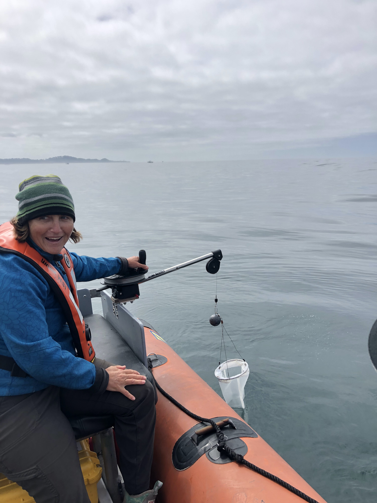
Since its start, the GEMM Lab has been interested in the effect of vessel disturbance on whales. From former student Florence’s masters project to Leila’s PhD work, this research has shown that gray whales on their foraging grounds have a behavioral response to vessel presence (Sullivan & Torres, 2018) and a physiological response to vessel noise (Lemos et al., 2022). Presently, our GRANITE project is continuing to investigate the effect of ambient noise on gray whales, with an emphasis on understanding how these effects might scale up to impact the population as a whole (Image 1).
To date, all this work has been focused on gray whales feeding off the coast of Oregon, but I’m excited to share that this is about to change! In just a few weeks, Leigh and I will be heading south for a pilot study looking at the effects of whale watching vessels on gray whale mom/calf pairs in the nursing lagoons of Baja California, Mexico.
Image 1. Infographic for the GRANITE project. Credit: Carrie Ekeroth
We are collaborating with a Fernanda Urrutia Osorio, a PhD candidate at Scripps Institute of Oceanography, to spend a week conducting fieldwork in one of the nursing lagoons. For this project we will be collecting drone footage of mom/calf pairs in both the presence and absence of whale watching vessels. Our goal is to see if we detect any differences in behavior when there are vessels around versus when there are not. Tourism regulations only allow the whale watching vessels to be on the water during specific hours, so we are hoping to use this regulated pattern of vessel presence and absence as a sort of experiment.
Image 2. A mom and calf pair. NOAA/NMFS permit #21678.
The lagoons are a crucial place for mom/calf pairs, this is where calves nurse and grow before migration, and nursing is energetically costly for moms. So, it is important to study disturbance responses in this habitat since any change in behavior caused by vessels could affect both the calf’s energy intake and the mom’s energy expenditure. While this hasn’t yet been investigated for gray whales in the lagoons, similar studies have been carried out on other species in their nursing grounds.
Video 1. Footage of “likely nursing” behavior. NOAA/NMFS permit #21678.
We can use these past studies as blueprints for both data collection and processing. Disturbance studies such as these look for a wide variety of behavioral responses. These include (1) changes in activity budgets, meaning a change in the proportion of time spent in a behavior state, (2) changes in respiration rate, which would reflect a change in energy expenditure, (3) changes in path, which would indicate avoidance, (4) changes in inter-individual distance, and (5) changes in vocalizations. While it’s not necessarily possible to record all of these responses, a meta-analysis of research on the impact of whale watching vessels found that the most common responses were increases in the proportion of time spent travelling (a change in activity budget) and increased deviation in path, indicating an avoidance response (Senigaglia et al., 2016).
One of the key phrases in all these possible behavioral responses is “change in ___”. Without control data collected in the absence of whale watching vessels, it impossible to detect a difference. Some studies have conducted controlled exposures, using approaches with the research vessel as proxies for the whale watchers (Arranz et al., 2021; Sprogis et al., 2020), while others use the whale watching operators’ daily schedule and plan their data collection schedule around that (Sprogis et al., 2023). Just as ours will, all these studies collected data using drones to record whale behavior and made sure to collect footage before, during, and after exposure to the vessel(s).
One study focused on humpback mom/calf pairs found a decrease in the proportion of time spent resting and an increase in both respiration rate and swim speed during the exposure (Sprogis et al., 2020). Similarly, a study focused on short-finned pilot whale mom/calf pairs found a decrease in the mom’s resting time and the calf’s nursing time (Arranz et al., 2021). And, Sprogis et al.’s study of Southern right whales found a decrease in resting behavior after the exposure, suggesting that the vessels’ affect lasted past their departure (Sprogis et al., 2023, Image 3). It is interesting that while these studies found changes in different response metrics, a common trend is that all these changes suggest an increase in energy expenditure caused by the disturbance.
However, it is important to note that these studies focused on short term responses. Long term impacts have not been thoroughly estimated yet. These studies provide many valuable insights, not only into the response of whales to whale watching, but also a look at the various methods used. As we prepare for our fieldwork, it’s useful to learn how other researchers have approached similar projects.
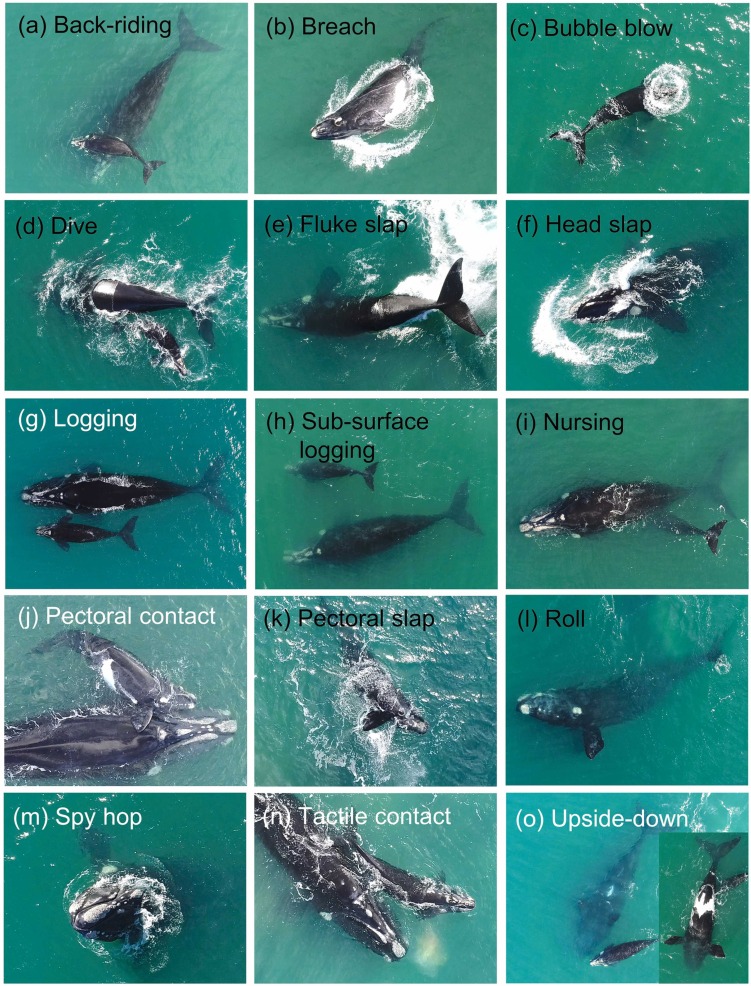
Image 3. Visual ethogram from Sprogis et al. 2023. This shows all the behaviors they identified from the footage.
I want to note that I don’t write this blog intending to condemn whale watching. I fully appreciate that offering the opportunity to view and interact with these incredible creatures is valuable. After all, it is one of the best parts of my job. But hopefully these disturbance studies can inform better regulations, such as minimum approach distances or maximum engine noise levels.
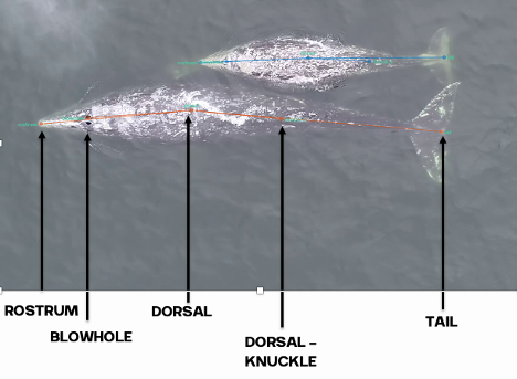
As these studies have done, our first step will be to establish an ethogram of behaviors (our list of defined behaviors that we will identify in the footage) using our pilot data. We can also record respiration and track line data. An additional response that I’m excited to add is the distance between the mom and her calf. Former GEMM Lab NSF REU intern Celest will be rejoining us to process the footage using the AI method she developed last summer (Image 4). As described in her blog, this method tracks a mom and calf pair across the video frames, and allows us to extract the distance between them. We look forward to adding this metric to the list and seeing what we can glean from the results.
Image 4. Example of a labelled frame from SLEAP, highlighting labels: rostrum, blowhole, dorsal, dorsal-knuckle, and tail. This labels are drawn to train the software to recognize the whales in unlabelled frames.
While we are just getting started, I am excited to see what we can learn about these whales and how best to study them. Stay tuned for updates from Baja!
Did you enjoy this blog? Want to learn more about marine life, research, and conservation? Subscribe to our blog and get a weekly alert when we make a new post! Just add your name into the subscribe box below!
References
Arranz, P., Glarou, M., & Sprogis, K. R. (2021). Decreased resting and nursing in short-finned pilot whales when exposed to louder petrol engine noise of a hybrid whale-watch vessel. Scientific Reports, 11(1), 21195. https://doi.org/10.1038/s41598-021-00487-0
Lemos, L. S., Haxel, J. H., Olsen, A., Burnett, J. D., Smith, A., Chandler, T. E., Nieukirk, S. L., Larson, S. E., Hunt, K. E., & Torres, L. G. (2022). Effects of vessel traffic and ocean noise on gray whale stress hormones. Scientific Reports, 12(1), Article 1. https://doi.org/10.1038/s41598-022-14510-5
Senigaglia, V., Christiansen, F., Bejder, L., Gendron, D., Lundquist, D., Noren, D., Schaffar, A., Smith, J., Williams, R., Martinez, E., Stockin, K., & Lusseau, D. (2016). Meta-analyses of whale-watching impact studies: Comparisons of cetacean responses to disturbance. Marine Ecology Progress Series, 542, 251–263. https://doi.org/10.3354/meps11497
Sprogis, K. R., Holman, D., Arranz, P., & Christiansen, F. (2023). Effects of whale-watching activities on southern right whales in Encounter Bay, South Australia. Marine Policy, 150, 105525. https://doi.org/10.1016/j.marpol.2023.105525
Sprogis, K. R., Videsen, S., & Madsen, P. T. (2020). Vessel noise levels drive behavioural responses of humpback whales with implications for whale-watching. ELife, 9, e56760. https://doi.org/10.7554/eLife.56760
Sullivan, F. A., & Torres, L. G. (2018). Assessment of vessel disturbance to gray whales to inform sustainable ecotourism. Journal of Wildlife Management, 82(5), 896–905. https://doi.org/10.1002/jwmg.21462
Reports of whale entanglements have been on the rise over the last decade on the US West Coast, with Dungeness crab fishing gear implicated in many cases (Feist et al., 2021; Samhouri et al., 2021; Santora et al., 2020). State agencies are responsible for managing this environmental issue that has implications both for the endangered whale sub-populations that are subject to entanglements, and for the fishing activities, which play an important social, cultural, and economic role for coastal communities. In Oregon, the Oregon Whale Entanglement Working Group (today the Oregon Entanglement Advisory Committee, facilitated by ODFW – Oregon Department of Fish and Wildlife) formed in 2017, tasked with developing options to reduce entanglement risk. The group members composed of managers, researchers and fishermen identified that a lack of information and understanding of whale distribution in Oregon waters was a significant knowledge gap of high priority.
In response, the GEMM Lab and its collaborators at ODFW developed the OPAL project (Overlap Predictions About Large whales, phase 1: 2018-2022). The first phase of the project (phase 1) was developed to 1) model and predict large whale distribution off the coast of Oregon in relation to dynamic environmental conditions, and 2) assess overlap with commercial crab fishing gear to inform conservation efforts. Although this first phase was extended up to June as a result of COVID, it is now coming to an end. As a postdoc in the GEMM Lab, I have been the main analyst working on this project. The habitat use models that I generated from several years of aerial and boat-based surveys provide improved knowledge about where and when rorqual whales (combining blue, humpback and fin) are most abundant (Derville et al., 2022). Moreover, we are about to publish an analysis of overlap between whale predicted densities and commercial Dungeness crab fishing effort. This analysis of co-occurrence over 10 years shows distinct spatio-temporal patterns in relation to climatic fluctuations affecting the northern California Current System (Derville et al., In review).
Although we are quite satisfied with the outputs of these four years of research, this is not the end of it! Project OPAL continues into a second phase (2022-2025; supported by NOAA Section 6 funding), during which models will be improved and refined via incorporation of new survey data (helicopter and boat-based) as well as prey data (krill and fish distribution). PhD student Rachel Kaplan is a key contributor to this research, and I will do my best to keep assisting her in this journey in the years to come.
Announcing SLATE!
As this newly acquired knowledge leads to potentially new management measures in Oregon, it becomes essential for managers to evaluate their impacts on the entanglement issue. But how do we know exactly how many entanglements occur during any year within Oregon waters? Is recording reports of entanglements or signs of entanglements in stranded whales enough? The simple answer is no. Entanglements are notoriously under-detected and under-reported (Tackaberry et al., 2022). Over the US West Coast, entanglements are also relatively rare events that can easily go unnoticed in the immensity of the ocean. Moreover, entangled large whales are often able to carry the fishing gear for some time away from the initial gearset location, which makes it hard to locate the origin of the gear causing problems (van der Hoop et al., 2017).
Figure 1: Graphical representation of the SLATE project representing the different tasks described below. Work in progress…
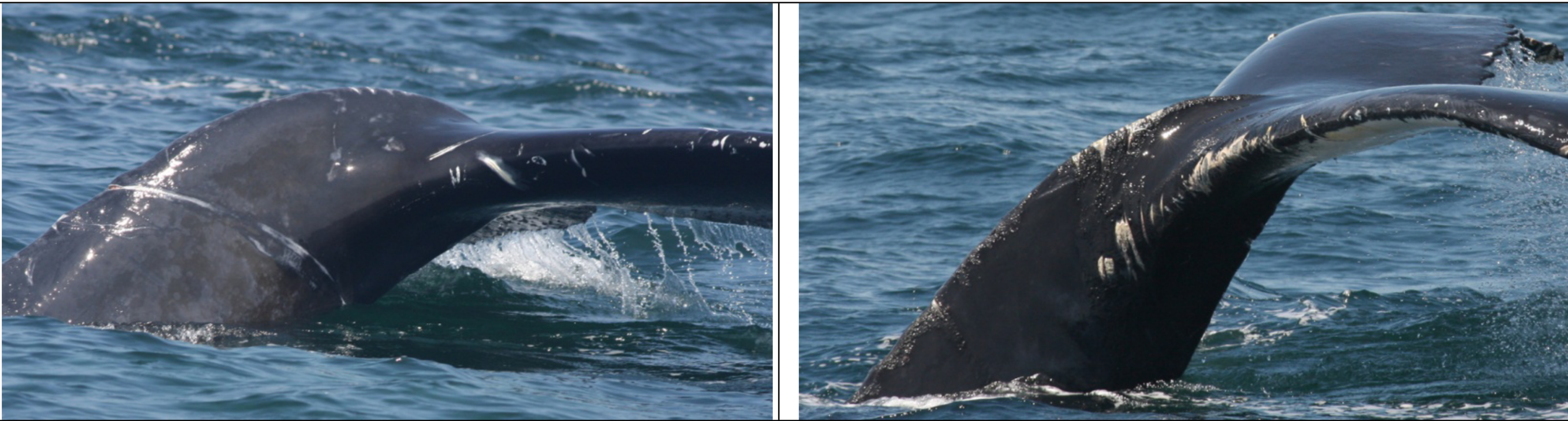
Our approach to the challenge of assessing humpback whale entanglement rates in Oregon waters is to use scar analysis. Our new “SLATE” (Scar-based Long-term Assessment of Trends in whale Entanglements, Figure 1) project will be using scar-based methods as a proxy to detect unobserved entanglement events (e.g., Basran et al., 2019; Bradford et al., 2009; George et al., 2017; Knowlton et al., 2012; Robbins, 2012). Indeed, this approach has been effective to detect potential interactions with fishing gear at a much higher frequency than entanglement reports in the Atlantic Ocean (e.g., only 10% of entanglements of humpback whales in the Gulf of Maine were estimated to be reported; Robbins, 2012). We will be examining hundreds of photographs of humpback whales observed in Oregon waters to try to detect wrapping scars and notches that result from entanglement events. Based on this scar pattern, we will assign each whale a qualitative probability of prior entanglement (i.e., uncertain, low, high). We will specifically be looking at the caudal peduncle (the attachment point of the whale’s fluke, see Figure 2) following a methodology developed in the Gulf of Maine by Robbins & Mattila, (2001).
Figure 2: Examples of unhealed injuries interpreted as entanglement related in 2010 in the Gulf of Maine. Figure reproduced from (Robbins, 2012).
Data please?
While this approach is to-date the most applicable way to assess otherwise undetected entanglements, it is sometimes limited by sample size. Although we plan to collect more photos in the field in summer 2023 and 2024, this long-term analysis of scarring patterns would not be possible without the contribution of the Cascadia Research Collective (CRC) led by John Calambokidis. The CRC humpback whale catalogue will be crucial to assessing entanglement rates at the individual level over the last decade.
Moreover, as we have been contemplating the task ahead of us, we realized that the data collected through traditional scientific surveys might not be sufficient to achieve our goal. We need the help of the people who live off the ocean and encounter whales on a day-to-day basis: fishermen. That is why we decided to solicit interested fishermen to take photographs of whales while at sea. Starting this year, we will work with at least three self-selected fishermen who are interested in supporting this program and collecting data to support the research efforts. Participants will be provided a stipend, equipped with a high-quality camera, and trained to photograph whales while following National Oceanic and Atmospheric Administration (NOAA) Marine Mammal Protection Act (MMPA) guidelines.
And here come the statistics…
If we have some of my previous blogs (e.g., May 2022, June 2018), you know that I usually participate in projects that have a significant statistical modeling component. As part of the SLATE project, I will be trying out some new approaches that I never had the opportunity to work with before, which makes me feels both super excited and slightly apprehensive!
First, I will analyze humpback whale scarring at the population level. That means I will be using all available photos of whales in Oregon waters without considering individual identification, and I will model the probability of entanglement scars in relation to space and time. This model will help us answer questions such as: did whales have a higher chance of becoming entangled in certain years over others? Did whales observed in a certain zone in Oregon waters have a higher risk of getting entangled?
Second, I will analyze humpback whale scarring at the individual level. This time, we will only use encounters of a selected number of individuals that have a long recapture history, meaning that they were photo-identified and resighted several times throughout the last decade. Using a genetic database produced by the Cetacean Conservation and Genomic Laboratory (CCGL, Marine Mammal Institute), we will also be able to tell to which “Distinct Population Segment” (DPS) some of these individual whales belong. Down the line, this is an important piece of information because humpback whale DPS do not breed in the same areas, and these groups have different levels of population health. Then, we will use what is known as a “multi-event mark-recapture model” to estimate the probability of entanglement as a function of time and spatial residency or DPS assignment, while accounting for detection probability and survival.
Through these analyses, our goal is to produce a single indicator to help managers assess the effects of mandatory or voluntary changes in Oregon fishing practices. In the end, we hope that these models will provide a measurable and robust way of monitoring whale entanglements in fishing gear off the coast of Oregon.
References
Basran, C. J., Bertulli, C. G., Cecchetti, A., Rasmussen, M. H., Whittaker, M., & Robbins, J. (2019). First estimates of entanglement rate of humpback whales Megaptera novaeangliae observed in coastal Icelandic waters. Endangered Species Research, 38(February), 67–77. https://doi.org/10.3354/ESR00936
Bradford, A. L., Weller, D. W., Ivashchenko, Y. v., Burdin, A. M., & Brownell, R. L. (2009). Anthropogenic scarring of western gray whales (Eschrichtius robustus). Marine Mammal Science, 25(1), 161–175. https://doi.org/10.1111/j.1748-7692.2008.00253.x
Derville, S., Barlow, D. R., Hayslip, C. E., & Torres, L. G. (2022). Seasonal, Annual, and Decadal Distribution of Three Rorqual Whale Species Relative to Dynamic Ocean Conditions Off Oregon, USA. Frontiers in Marine Science, 9, 1–19. https://doi.org/10.3389/fmars.2022.868566
Derville, S., Buell, T., Corbett, K., Hayslip, C., & Torres, L. G. (n.d.). Exposure of whales to entanglement risk in Dungeness crab fish-ing gear in Oregon, USA, reveals distinctive spatio-temporal and climatic patterns. Biological Conservation.
Feist, B. E., Samhouri, J. F., Forney, K. A., & Saez, L. E. (2021). Footprints of fixed-gear fisheries in relation to rising whale entanglements on the U.S. West Coast. Fisheries Management and Ecology, 28(3), 283–294. https://doi.org/10.1111/fme.12478
George, J. C., Sheffield, G., Reed, D. J., Tudor, B., Stimmelmayr, R., Person, B. T., Sformo, T., & Suydam, R. (2017). Frequency of injuries from line entanglements, killer whales, and ship strikes on bering-chukchi-beaufort seas bowhead whales. Arctic, 70(1), 37–46. https://doi.org/10.14430/arctic4631
Knowlton, A. R., Hamilton, P. K., Marx, M. K., Pettis, H. M., & Kraus, S. D. (2012). Monitoring North Atlantic right whale Eubalaena glacialis entanglement rates: A 30 yr retrospective. Marine Ecology Progress Series, 466(Kraus 1990), 293–302. https://doi.org/10.3354/meps09923
Robbins, J. (2012). Scar-Based Inference Into Gulf of Maine Humpback Whale Entanglement : 2010 (Issue January). Report to the Northeast Fisheries Science Center National Marine Fisheries Service, EA133F09CN0253 Item 0003AB, Task 3.
Robbins, J., & Mattila, D. K. (2001). Monitoring entanglements of humpback whales ( Megaptera novaeangliae ) in the Gulf of Maine on the basis of caudal peduncle scarring. SC/53/NAH25. Report to the Scientific Committee of the International Whaling Commission, 14, 1–12. http://www.ccbaymonitor.org/pdf/scarring.pdf
Samhouri, J. F., Feist, B. E., Fisher, M. C., Liu, O., Woodman, S. M., Abrahms, B., Forney, K. A., Hazen, E. L., Lawson, D., Redfern, J., & Saez, L. E. (2021). Marine heatwave challenges solutions to human-wildlife conflict. Proceedings of the Royal Society B: Biological Sciences, 288, 20211607. https://doi.org/10.1098/rspb.2021.1607
Santora, J. A., Mantua, N. J., Schroeder, I. D., Field, J. C., Hazen, E. L., Bograd, S. J., Sydeman, W. J., Wells, B. K., Calambokidis, J., Saez, L., Lawson, D., & Forney, K. A. (2020). Habitat compression and ecosystem shifts as potential links between marine heatwave and record whale entanglements. Nature Communications, 11, 536. https://doi.org/10.1038/s41467-019-14215-w
Tackaberry, J., Dobson, E., Flynn, K., Cheeseman, T., Calambokidis, J., & Wade, P. R. (2022). Low Resighting Rate of Entangled Humpback Whales Within the California , Oregon , and Washington Region Based on Photo-Identification and Long-Term Life History Data. Frontiers in Marine Science, 8(January), 1–13. https://doi.org/10.3389/fmars.2021.779448
van der Hoop, J., Corkeron, P., & Moore, M. (2017). Entanglement is a costly life-history stage in large whales. Ecology and Evolution, 7(1), 92–106. https://doi.org/10.1002/ece3.2615
ByRachel Kaplan, PhD student, OSU College of Earth, Ocean and Atmospheric Sciences and Department of Fisheries, Wildlife, & Conservation Sciences, Geospatial Ecology of Marine Megafauna Lab
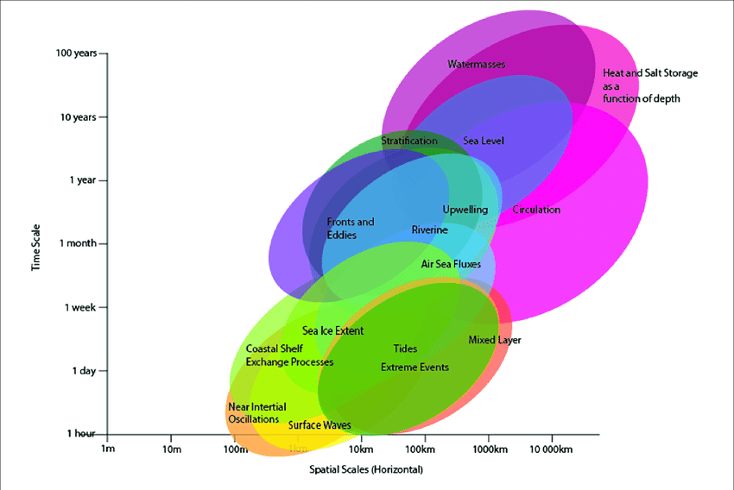
Ocean ecosystems are complex and dynamic, shaped by the interconnected physical and biogeochemical processes that operate across a variety of timescales. A trip on the “ocean conveyer belt”, which transports water from the North Atlantic across the global ocean and back in a process called thermohaline circulation, takes about a thousand years to complete. Phytoplankton blooms, which cycle nutrients through the surface ocean and feed marine animals, often occur at the crucial, food-poor moment of spring, and last for weeks or months. The entanglement of a whale in fishing gear, a major anthropogenic threat to ocean life that drives the GEMM Lab’s Project OPAL, can happen in seconds.
Compounding this complexity, even the timescales that research has clarified are changing. Many processes in the ocean are shifting – and often accelerating – due to global climate change. Images of melting sea ice, calving glaciers, and coastal erosion all exemplify our natural world’s rapid reorganization, and even discrete events can have dramatic repercussions and leave their mark for years. For example, a marine heatwave that occurred in 2014-2015 raised temperatures up to 2.5° C warmer than usual, redistributed species northward along the United States’ West Coast, spurred harmful algal blooms, and shut down fisheries. The toxic blooms also caused marine mammal strandings, domoic acid poisoning in California sea lions, and seabird mass death events (McCabe et al., 2016).
Figure 1. Figures like this Stommel diagram reveal the broad temporal and spatial scales over which ocean phenomena occur. Source: Sloyan et al., 2019
As humans seek to manage ocean ecosystems and mitigate the effects of climate change, our political processes have their own time scales, interconnected cycles, and stochasticity, just like the ocean. At the federal level in the United States, the legislative process takes place over months to decades, sometimes punctuated by relatively quicker actions enacted through Executive Orders. In addition, just as plankton have their turnover times, so do governmental branches. Both the legislative branch and the executive branch change frequently, with new members of Congress coming in every two years, and the president and administration changing every four or eight years. Turnover in both of these branches may constitute a total regime shift, with new members seeking to redirect science policy efforts.
The friction between oceanic and political timescales has historically made crafting effective ocean conservation policy difficult. In recent years, the policy approach of “adaptive management” has sought to respond to the challenges at the tricky intersection of politics, climate change, and ocean ecosystems. The U.S. Department of the Interior’s Technical Guide to Adaptive Management highlights its capacity to deal with the uncertainty inherent to changing ecosystems, and its ability to accommodate progress made through research: “Adaptive management [is a decision process that] promotes flexible decision making that can be adjusted in the face of uncertainties as outcomes from management actions and other events become better understood. Careful monitoring of these outcomes both advances scientific understanding and helps adjust policies or operations as part of an iterative learning process” (Williams et al, 2009).
Over the last several years, adaptive management policy approaches have been key as resource managers along the West Coast have responded to the problem of whale entanglement in fishing gear. When the 2014-2015 marine heatwave event caused anomalously low krill abundance in the central California Current region, humpback whales used a tactic called “prey-switching”, and fed on inshore anchovy schools rather than offshore krill patches. The resulting habitat compression fueled an increase in humpback whale entanglement events in Dungeness crab fishing gear (Santora et al, 2020).
This sudden uptick in whale entanglements necessitated strategic management responses along the West Coast. In 2017, the California Dungeness Crab Fishing Gear Working Group developed the Risk Assessment and Mitigation Program (RAMP) to analyze real-time whale distribution and ocean condition data during the fishing season, and provide contemporaneous assessments of entanglement risk to the state’s Department of Fish and Wildlife. The Oregon Whale Entanglement Working Group (OWEWG) formed in 2017, tasked with developing options to reduce risk. Oregon Department of Fish and Wildlife (ODFW) has guided whale entanglement reduction efforts by identifying four areas of ongoing work: accountability, risk reduction, best management practices, and research – with regular, scheduled reviews of the regulations and opportunities to update and adjust them.
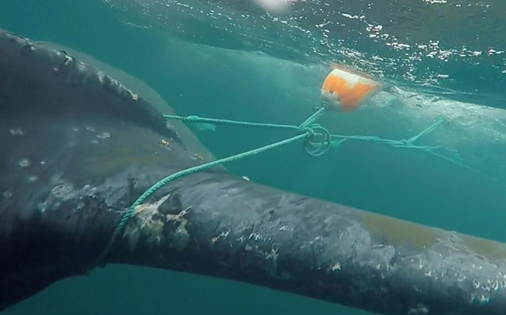
Figure 2. Entanglement in fishing gear can occur in seconds and may negatively impact whales for years. Source Scott Benson/NOAA
The need for research to support the best possible policy is where the GEMM Lab comes in. ODFW has established partnerships with Oregon State University and Oregon Sea Grant in order to improve understanding of whale distributions along the coast that can inform management efforts. Being involved in this cooperative “iterative learning process” is exactly why I’m so glad to be part of Project OPAL. Initial results from this work have already shaped ODFW’s regulations, and the framework of adaptive management and assessment means that regulations can continue being updated as we learn more through our research.
Ecosystem management will always be complex, just like ecosystems themselves. Today, the pace at which the climate is changing causes many people concern and even despair (Bryndum-Buchholz, 2022). Building adaptive approaches into marine policymaking, like the ones in use off the West Coast, introduces a new timescale into the U.S. policy cycle – one more in line with the rapid changes that are occurring within our dynamic ocean.
References
Williams, B. L., Szaro, R. C., and Shapiro, C. D. 2009. Adaptive management: the U.S. Department of the Interior Technical Guide. Adaptive Management Working Group, v pp.
Bryndum-Buchholz, A. (2022). Keeping up hope as an early career climate-impact scientist. ICES Journal of Marine Science, 79(9), 2345–2350. https://doi.org/10.1093/icesjms/fsac180
McCabe, R. M., Hickey, B. M., Kudela, R. M., Lefebvre, K. A., Adams, N. G., Bill, B. D., Gulland, F. M., Thomson, R. E., Cochlan, W. P., & Trainer, V. L. (2016). An unprecedented coastwide toxic algal bloom linked to anomalous ocean conditions. Geophys Res Lett, 43(19), 10366–10376. https://doi.org/10.1002/2016GL070023
Santora, J. A., Sydeman, W. J., Schroeder, I. D., Wells, B. K., & Field, J. C. (2011). Mesoscale structure and oceanographic determinants of krill hotspots in the California Current: Implications for trophic transfer and conservation. Progress in Oceanography, 91(4), 397–409. https://doi.org/10.1016/j.pocean.2011.04.002
Sloyan, B. M., Wilkin, J., Hill, K. L., Chidichimo, M. P., Cronin, M. F., Johannessen, J. A., Karstensen, J., Krug, M., Lee, T., Oka, E., Palmer, M. D., Rabe, B., Speich, S., von Schuckmann, K., Weller, R. A., & Yu, W. (2019). Evolving the Physical Global Ocean Observing System for Research and Application Services Through International Coordination. Frontiers in Marine Science, 6, 449. https://doi.org/10.3389/fmars.2019.00449
In October 1972, the tides turned for U.S. environmental politics: the Marine Mammal Protection Act (MMPA) was passed. Its creation ushered in a new flavor of conservation and management. With phrases like “optimum sustainable population” baked into its statutory language, it marked among the first times that ecosystem-based management — an approach which directly calls upon knowledge of ecology to inform action — was required by law (Ray and Potter 2022). Transitioning from reductionist, species-siloed policies, the MMPA instead placed the interdependency of species at the core of ecosystem function and management.
Beyond deepening the role of science on Capitol Hill, the MMPA’s greatest influence may have been spurred by the language that prohibited “the taking and importation of marine mammals” (16 U.S.C. 1361). Because the word “taking” is multivalent, it carries on its back many interpretations. “Taking” a marine mammal is not limited to intentionally hunting or killing them, or even accidental bycatch. “Taking” also includes carelessly operating a boat when a marine mammal is present, feeding a marine mammal in the wild, or tagging a marine mammal without the appropriate scientific permit. “Taking” a marine mammal can also extend to the fatal consequences caused by noise pollution — not intent, but incident (16 U.S.C. 1362).
The latter circumstances remain reverberant for the U.S. Navy. To comply with the MMPA, they are granted “incidental, but not intentional, taking of small numbers of marine mammals….[when] engag[ing] in a specified activity (other than commercial fishing)” (87 FR 33113). So, if the sonar activities required for national security exercises adversely impact marine mammals, the Navy has a bit of leeway but is still expected to minimize this impact. To further mitigate this potential harm, the Navy thus invests heavily in marine mammal research. (If you are interested in learning more about how the Navy has influenced the trajectory of oceanographic research more broadly, you may find this book interesting.)
Beaked whales are an example of a marine mammal we know much about due to the MMPA’s call for research when incidental take occurs. Three decades ago, many beaked whales stranded ashore following a series of U.S. Navy sonar exercises. Since then, the Navy has flooded research dollars toward better understanding beaked whale hearing, vocal behavior, and movements (e.g., Klinck et al. 2012). Through these efforts, a deluge of research charged with developing effective tools to acoustically monitor and conserve beaked whales has emerged.
These studies have laid the foundation for my Ph.D. research, which is dedicated to the Holistic Assessment of Living marine resources off Oregon (HALO) project. Through both visual and acoustic surveys, the HALO project’s mission is to understand how changes in ocean conditions — driven by global climate change — influence living marine resources in Oregon waters.
In my research specifically, I aim to learn more about beaked whales off the Oregon coast. Beaked whales represent nearly a fourth of cetacean species alive today, with at least 21 species recorded to date (Roman et al. 2013). Even so, 90% of beaked whales are considered data deficient: we lack enough information about them to confidently describe the state of their populations or decide upon effective conservation action.
Much remains to be learned about beaked whales, and I aim to do so by eavesdropping on them. By referring to the “acoustic repertoire” of beaked whales — that is, their vocalizations and corresponding behaviors — I aim to tease out their vocalizations from the broader ocean soundscape and understand how their presence in Oregon waters varies over time.
Beaked whales are notoriously cryptic, elusive to many visual survey efforts like those aboard HALO cruises. In fact, some species have only been identified via carcasses that have washed ashore (Moore and Barlow 2013). Acoustic studies have elucidated ecological information (beaked whales forage at night at seamounts summits; Johnston et al. 2008) and have also introduced promising population-level monitoring efforts (beaked whales have been acoustically detected in areas with a historical scarcity of sightings; Kowarski et al. 2018). Their deep-diving nature often renders them inconspicuous, and they forage at depths between 1,000 and 2,000 m, on dives as long as 90 minutes (Moore and Barlow 2013; Klinck et al. 2012). Their echolocation clicks are produced at frequencies within the hearing range of killer whales, and previous studies have suggested that Blainville’s beaked whales are only vocally active during deep foraging dives and not at the surface, possibly to prevent being acoustically detected by predatory killer whales. Researchers refer to this phenomenon as “acoustic crypsis,” or when vocally-active marine mammals are strategically silent to avoid being found by potential predators (Aguilar de Soto et al. 2012).
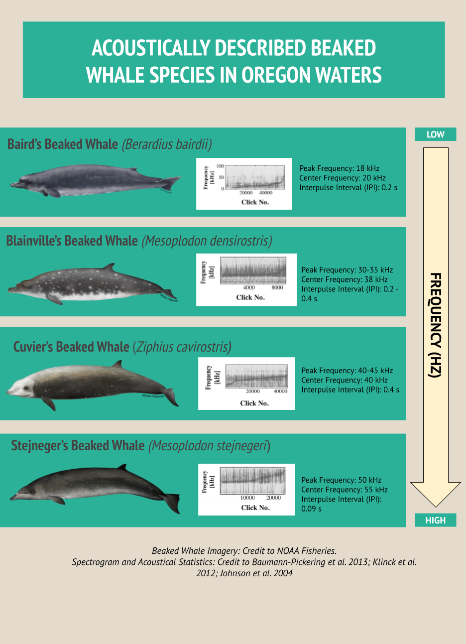
We expect to see evidence of Blainville’s beaked whales in Oregon waters, as well as Baird’s, Cuvier’s, Stejneger’s, Hubb’s, and other beaked whale species. Species-specific echolocation clicks were comprehensively described a decade ago in Baumann-Pickering et al. 2013 (Figure 1). While this study laid the groundwork for species-level beaked whale acoustic detection, much more work is still needed to describe their acoustic repertoire with higher resolution detail. For example, though Hubb’s beaked whales live in Oregon waters, their vocal behavior remains scantly defined.
Figure 1: Baird’s, Blainville’s, Cuvier’s, and Stejneger’s beaked whales are among the most comprehensively acoustically described beaked whales inhabiting central Oregon waters, though more work would improve accuracy in species-specific acoustic detection. Credit: Marissa Garcia. Infographic draws upon beaked whale imagery from NOAA Fisheries and spectrograms and acoustical statistics published in Baumann-Pickering et al. 2013.
The HALO project seeks to add a biological dimension to the historical oceanographic studies conducted along the Newport Hydrographic (NH) line ever since the 1960s (Figure 2). Rockhopper acoustic recording units are deployed at sites NH 25, NH 45, and NH 65. The Rockhopper located at site NH 65 is actively recording on the seafloor about 2,800 m below the surface. Because beaked whales tend to be most vocally active at these deep depths, we will first dive into the acoustic data on NH 65, our deepest unit, in hopes of finding beaked whale recordings there.
Figure 2: The HALO project team conducts quarterly visual surveys along the NH line, spanning between NH 25 and NH 65. Rockhopper acoustic recording units continuously record at the NH 25, NH 45, and NH 65 sites. Credit: Leigh Torres.
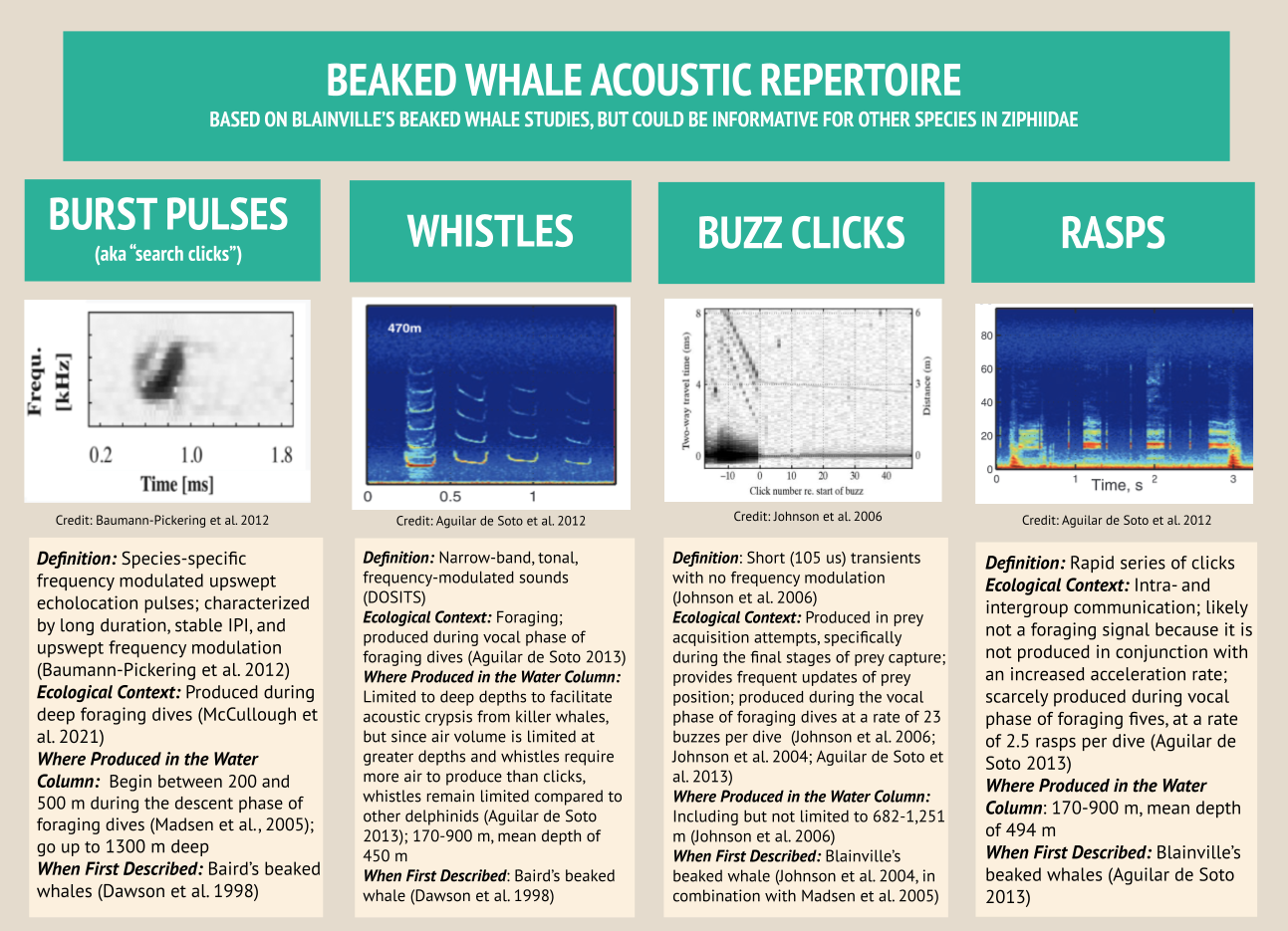
Beaked whales’ acoustic repertoire can be broadly split into four primary categories: burst pulses (aka “search clicks”), whistles, buzz clicks, and rasps. Beaked whale search clicks, which are regarded as burst pulses when produced in succession, have distinct qualities: their upswept frequency modulation (meaning the frequency gets higher within the click), their long duration especially when compared to other delphinid clicks, and a consistent interpulse interval which is the time of silence between signals (Baumann-Pickering et al. 2013). Acoustic analysts can identify different species based on how the frequency changes in different burst pulse sequences (Baumann-Pickering et al. 2013; Figure 1). For this reason, when I conduct my HALO analyses, I intend to automatically detect beaked whale species using burst pulses, as they are the best documented beaked whale signal, with unique signatures for each species.
In the landscape of beaked whale acoustics, the acoustic repertoire of Blainville’s beaked whales (Mesoplodon densirostris) — a species of focus in my HALO analyses — is especially well defined. Blainville’s beaked whale whistles have been recorded up to 900 m deep, representing the deepest whistle recorded for any marine mammal to date in the literature (Aguilar de Soto et al. 2012). While Blainville’s beaked whales only spend 40% of their time at depths below 170 m, two key vocalizations occur at these depths: whistles and rasps. While they remain surprisingly silent near the surface, beaked whales produce whistles and rasps at depths up to 900 m. The beaked whales dive together in synchrony, and right before they separate from each other, they produce the most whistles and rasps, further indicating that these vocalizations are used to enhance foraging success (Aguilar de Soto et al. 2006). As beaked whales transition to foraging on their own, they predominantly produce frequently modulated clicks and buzzes. Beaked whales produce buzzes in the final stages of prey capture to receive up-to-date information about their prey’s location. The buzzes’ high repetition enables the whale to achieve 300+ updates on their intended prey’s location in the last 3 m before seizing their feast (Johnson et al. 2006; Figure 3).
Figure 3: Blainville’s beaked whales generally have four categories within their acoustic repertoire, including burst pulses, whistles, buzz clicks, and rasps. Credit: Marissa Garcia.
All of this knowledge about beaked whale acoustics can be linked back to the MMPA, which has also achieved broader success. Since the MMPA’s implementation, marine mammal population numbers have risen across the board. For marine mammal populations with sufficient data, approximately 65% of these stocks are increasing and 17% are stable (Roman et al. 2013).
Nevertheless, perhaps much of the MMPA’s true success lies in the research it has indirectly fueled, by virtue of the required compliance of governmental bodies such as the U.S. Navy. And the response has proven to be a boon to knowledge: if the U.S. Navy has been the benefactor of marine mammal research, beaked whale acoustics has certainly been the beneficiary. We hope the beaked whale acoustic analyses stemming from the HALO Project can further this expanse of what we know.
References
Aguilar de Soto, N., Madsen, P. T., Tyack, P., Arranz, P., Marrero, J., Fais, A., Revelli, E., & Johnson, M. (2012). No shallow talk: Cryptic strategy in the vocal communication of Blainville’s beaked whales. Marine Mammal Science, 28(2), E75–E92. https://doi.org/10.1111/j.1748-7692.2011.00495.x
Baumann-Pickering, S., McDonald, M. A., Simonis, A. E., Solsona Berga, A., Merkens, K. P. B., Oleson, E. M., Roch, M. A., Wiggins, S. M., Rankin, S., Yack, T. M., & Hildebrand, J. A. (2013). Species-specific beaked whale echolocation signals. The Journal of the Acoustical Society of America, 134(3), 2293–2301. https://doi.org/10.1121/1.4817832
Johnston, D. W., McDonald, M., Polovina, J., Domokos, R., Wiggins, S., & Hildebrand, J. (2008). Temporal patterns in the acoustic signals of beaked whales at Cross Seamount. Biology Letters (2005), 4(2), 208–211. https://doi.org/10.1098/rsbl.2007.0614
Johnson, M., Madsen, P. T., Zimmer, W. M. X., de Soto, N. A., & Tyack, P. L. (2004). Beaked whales echolocate on prey. Proceedings of the Royal Society. B, Biological Sciences, 271(Suppl 6), S383–S386. https://doi.org/10.1098/rsbl.2004.0208
Johnson, M., Madsen, P. T., Zimmer, W. M. X., de Soto, N. A., & Tyack, P. L. (2006). Foraging Blainville’s beaked whales (Mesoplodon densirostris) produce distinct click types matched to different phases of echolocation. Journal of Experimental Biology, 209(Pt 24), 5038–5050. https://doi.org/10.1242/jeb.02596
Klinck, H., Mellinger, D. K., Klinck, K., Bogue, N. M., Luby, J. C., Jump, W. A., Shilling, G. B., Litchendorf, T., Wood, A. S., Schorr, G. S., & Baird, R. W. (2012). Near-real-time acoustic monitoring of beaked whales and other cetaceans using a Seaglider. PloS One, 7(5), e36128. https://doi.org/10.1371/annotation/57ad0b82-87c4-472d-b90b-b9c6f84947f8
Kowarski, K., Delarue, J., Martin, B., O’Brien, J., Meade, R., Ó Cadhla, O., & Berrow, S. (2018). Signals from the deep: Spatial and temporal acoustic occurrence of beaked whales off western Ireland. PloS One, 13(6), e0199431–e0199431. https://doi.org/10.1371/journal.pone.0199431
Madsen, P. T., Johnson, M., de Soto, N. A., Zimmer, W. M. X., & Tyack, P. (2005). Biosonar performance of foraging beaked whales (Mesoplodon densirostris). Journal of Experimental Biology, 208(Pt 2), 181–194. https://doi.org/10.1242/jeb.01327
McCullough, J. L. K., Wren, J. L. K., Oleson, E. M., Allen, A. N., Siders, Z. A., & Norris, E. S. (2021). An Acoustic Survey of Beaked Whales and Kogia spp. in the Mariana Archipelago Using Drifting Recorders. Frontiers in Marine Science, 8. https://doi.org/10.3389/fmars.2021.664292
Moore, J. E. & Barlow, J. P. (2013). Declining abundance of beaked whales (family Ziphiidae) in the California Current large marine ecosystem. PloS One, 8(1), e52770–e52770. https://doi.org/10.1371/journal.pone.0052770
Ray, G. C. & Potter, F. M. (2011). The Making of the Marine Mammal Protection Act of 1972. Aquatic Mammals, 37(4), 522.
Roman, J., Altman, I., Dunphy-Daly, M. M., Campbell, C., Jasny, M., & Read, A. J. (2013). The Marine Mammal Protection Act at 40: status, recovery, and future of U.S. marine mammals. Annals of the New York Academy of Sciences, 1286(1), 29–49. https://doi.org/10.1111/nyas.12040
Models can be extremely useful tools to describe biological systems and answer ecological questions, but they are often tricky to construct. If I have learned anything in my statistics classes, it is the importance of resisting the urge to throw everything but the kitchen sink into a model. However, this is usually much easier said than done, and model construction takes a lot of practice. The principle of simplicity is currently at the forefront of my thesis work, as I try to embody the famous quote by Albert Einstein:
“Everything should be made as simple as possible, but no simpler.”
As you might remember from my earlier blog, the goal of my thesis is to use biologging data to define different foraging behaviors of Pacific Coast Feeding Group (PCFG) gray whales, and then calculate the energetic cost of those behaviors. I am defining PCFG foraging behaviors at two scales: (1) dives that represent different behavior states (e.g., travelling vs foraging), and (2) roll events, which are periods during dives where the whale is rolled onto their side, that represent different foraging tactics (e.g., headstanding vs side-swimming).
Initially, I was planning to use a clustering analysis to define these different foraging behaviors at both the dive and roll event scale, as this method has been used to successfully classify different foraging strategies for Galapagos sea lions (Schwarz et al., 2021). In short, this clustering analysis uses summary variables from events of interest to group events based on their similarity. These can be any metric that describes the event such as duration and depth, or body positioning variables like median pitch or roll. The output of the clustering analysis method results in groups of events that can each be used to define a different behavior.
However, while this method works for defining the foraging tactics of PCFG gray whales, my discussions with other scientists have suggested that there is a better method available for defining foraging behavior at the dive scale: Hidden Markov Models (HMMs). HMMs are similar to the clustering method described above in that they use summary variables at discrete time scales to define behavior states, but HMMs take into account the bias inherent to time series data – events that occur closer together in time are more likely to be more similar. This bias of time can confound clustering analyses, making HMMs a better tool for classifying a series of dives into different behavior states.
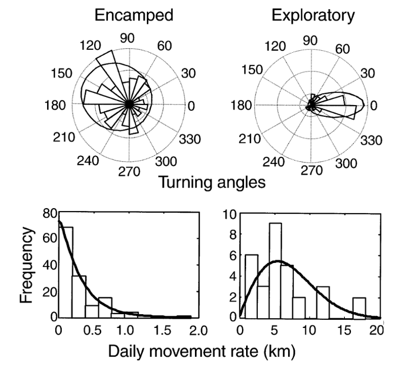
Like many analytical methods, the HMM framework was first proposed in a terrestrial system where it was used to classify the movement of translocated elk (Morales et al., 2004). The initial framework proposed using the step length, or the spatial distance between the animal’s locations at the start of subsequent time intervals, and the corresponding turning angle, to isolate “encamped” from “exploratory” behaviors in each elk’s movement path (Figure 1, from Morales et al., 2004). “Encamped” behaviors are those with short step lengths and high turning angles that show the individual is moving within a small area, and they can be associated with foraging behavior. On the other hand, “exploratory” behaviors are those with long step lengths and low turning angles that show the individual is moving in a relatively straight path and covering a lot of ground, which is likely associated with travelling behavior.
Figure 1. The difference between “encamped” and “exploratory” behavior states from a simple Hidden Markov Model (HMM) in a translocated elk equipped with a GPS collar (Fig. 1 in Morales et al., 2004). The top rose plots show the turning angles while the bottom histograms show the step lengths as a daily movement rate. The “encamped” state has short step lengths (low daily movement rate) and high turning angles while the “exploratory” state has long step lengths (high daily movement rate) and low turning angle. These behavior states from the HMM can then be interpollated to elk behavior, as the low daily movement and tight turns of the “encamped” behavior state likely indicates foraging while the high daily movement and direct path of the “exploratory” behavior state likely indicates traveling. Thus, it is important to keep the biological relevance of the study system in mind while constructing and interpreting the model.
In the two decades following this initial framework proposed by Morales et al. (2004), the use of HMMs in anlaysis has been greatly expanded. One example of this expansion has been the development of mutlivariate HMMs that include additional data streams to supplement the step length and turning angle classification of “encamped” vs “exploratory” states in order to define more behaviors in movement data. For instance, a multivariate HMM was used to determine the impact of acoustic disturbance on blue whales (DeRuiter et al., 2017). In addition to step length and turning angle, dive duration and maximum depth, the duration of time spent at the surface following the dive, the number of feeding lunges in the dive, and the variability of the compass direction the whale was facing during the dive were all used to classify behavior states of the whales. This not only allowed for more behavior states to be identified (three instead of two as determined in the elk model), but also the differences in behavior states between individual animals included in the study, and the differences in the occurrence of behavior states due to changes in environmental noise.
The mutlivariate HMM used by DeRuiter et al. (2017) is a model I would ideally like to emulate with the biologging data from the PCFG gray whales. However, incorporating more variables invites more questions during the model construction process. For example, how many variables should be incorporated in the HMM? How should these variables be modeled? How many behavior states can be identified when including additional variables? These questions illustrate how easy it is to unnecessarily overcomplicate models and violate the principle of simiplicity toted by Albert Einstein, or to be overwhelmed by the complexity of these analytical tools.
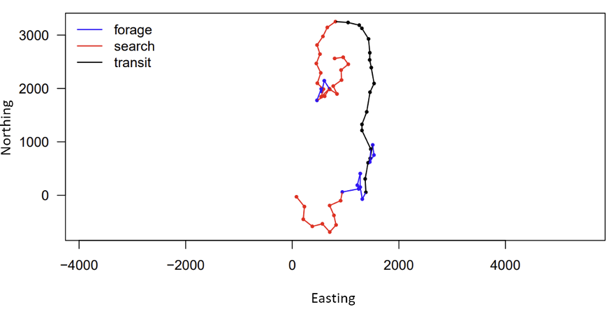
Figure 2. Example of expected output of Hidden Markov Model (HMM) for the PCFG gray whale biologging data (GEMM Lab; National Marine Fisheries Service (NMFS) permit no. 21678). The figure shows the movement track the whale swam during the deployment of the biologger, with each point representing the start of a dive. The axes show “Easting” and “Northing” rather than map coordinates because this is the relative path the whale took rather than GPS coordinates of the whale’s location. Each color represents a different behavior state—blue has short step lengths and high turning angles (likely foraging), red has intermediate step lengths and turning angles (likely searching), and black has long step lengths and low turning angles (likely transiting). These results will be refined as I construct the multivariate HMM that will be used in my thesis.
Luckily, I can draw on the support of Gray whale Response to Ambient Noise Informed by Technology and Ecology (GRANITE) project collaborators Dr. Leslie New and Dr. Enrico Pirotta to guide my HMM model construction and assist in interpreting the outputs (Figure 2). With their help, I have been learning the importance of always asking if the change I am making to my model is biologically relevent to the PCFG gray whales, and if it will help give me more insight into the whales’ behavior. Even though using complex tools, such as Hidden Markov Models, has a steep learning curve, I know that this approach is not only placing this data analysis at the cutting edge of the field, but helping me practice fundamental skills, like model construction, that will pay off down the line in my career.
Sources
DeRuiter, S. L., Langrock, R., Skirbutas, T., Goldbogen, J. A., Calambokidis, J., Friedlaender, A. S., & Southall, B. L. (2017). A multivariate mixed Hidden Markov Model for blue whale behaviour and responses to sound exposure. Annals of Applied Statistics, 11(1), 362–392. https://doi.org/10.1214/16-AOAS1008
Morales, J. M., Haydon, D. T., Frair, J., Holsinger, K. E., & Fryxell, J. M. (2004). Extracting more out of relocation data: Building movement models as mixtures of random walks. Ecology, 85(9), 2436–2445. https://doi.org/10.1890/03-0269
Schwarz, J. F. L., Mews, S., DeRango, E. J., Langrock, R., Piedrahita, P., Páez-Rosas, D., & Krüger, O. (2021). Individuality counts: A new comprehensive approach to foraging strategies of a tropical marine predator. Oecologia, 195(2), 313–325. https://doi.org/10.1007/s00442-021-04850-w
By Abby Tomita, undergraduate student, OSU College of Earth, Ocean, and Atmospheric Sciences
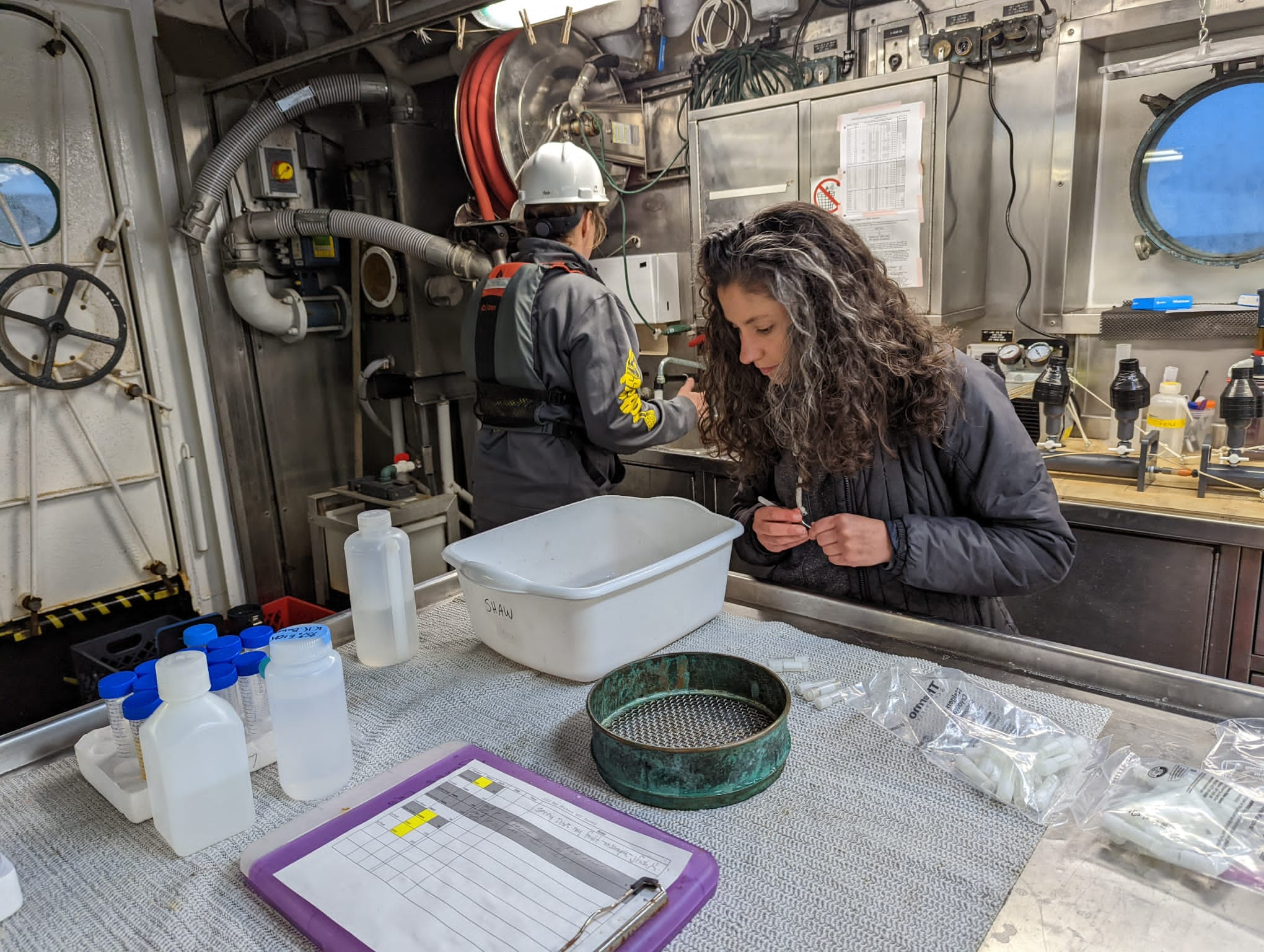
From long days in Newport performing the patience-testing task of bomb calorimetry, to spending hours transfixed by the microscopic world that exists in our oceans, I recently got an amazing glimpse into the world of marine biological research working with PhD student Rachel Kaplan. She has been an amazing teacher to my fellow intern Hadley and I, showing us the basics of the research process and introducing us to so many wonderful people at NOAA and the GEMM Lab. I am in my third year studying oceanography here at OSU and had no real lab experience before this, so I was eager to explore this area of research, and not only learn new information about our oceans, but also to see the research process up close and personal.
After being trained by Jennifer Fisher, a NOAA Research Fisheries Biologist, I sorted through zooplankton samples collected on the R/V Bell M. Shimada from the Northern California Current region. This data will be used to get an idea of where krill are found throughout the year, and in what abundances. Though my focus was mainly on two species of krill, I also found an assortment of other organisms, such as larval fish, squid, copepods, crabs, and tons of jellies, which were super interesting to see.
A small group of larval squid and other unknown species (photo by Abby Tomita).
I also studied krill through a technique called bomb calorimetry, which is not for the faint of heart! It takes a tough soul to be able to put these complex little creatures into a mortar and pestle and grind them into a dust that hits your nose like pepper. They then take their final resting place into the bomb calorimetry machine (which can and will find something to fuss over) until it finally manages to ignite and dispose of the krill’s remains. The light that guided me through this dark tunnel was the knowledge that these sacrificial krill were taken in the name of science, with the aim of eventually decreasing whale entanglements.
Abby placing the pellet within the coil for the bomb.
That, and Rachel’s contagious positivity. In the early stages, we would spend the majority of our time troubleshooting after constant “misfires”, in which the machine fails to combust the sample properly. Bomb calorimetry involves many tedious steps, and working with such small quantities of tissue – a single krill could weigh 0.01 grams or even less – poses a plethora of its own challenges. One of my biggest takeaways from this experience was to have patience with this kind of work and know when to take a much-needed dance break. Things often do not work out according to plan, and getting to see first-hand how to adapt to confounding variables and hitches in the procedure was an invaluable lesson.
I also got to see how collaborative the research process is. We received helpful advice from other members of the GEMM Lab at lunch, as well as constant help from our esteemed Resident Bomb Cal Expert, Elizabeth Daly. It was comforting for me to see that even when you are doing independent research, you are not expected to only work alone, and there can be so much community in higher level research.
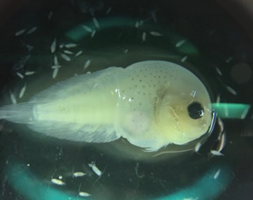
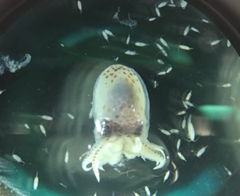
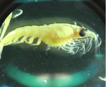
A larval snailfish.A larval fish (sp. unknown) still in its egg.A larval octopus. Female Thysanoessa spinifera krill (photos by Abby Tomita).
Did you enjoy this blog? Want to learn more about marine life, research, and conservation? Subscribe to our blog and get a weekly message when we post a new blog. Just add your name and email into the subscribe box below.
Another year has come and gone, and with the final days of 2022 upon us, it is my honor and pleasure to present to you, dear reader, this summary of achievements by the GEMM Lab this year. It has been another big year for us, so snuggle up with your favorite holiday drink and enjoy our recap of 2022!
Leigh working hard during GRANITE field work
2022 was a huge year of milestones for each lab member. The biggest happened just a few weeks ago when, on December 1st, our primary investigator (PI) and the captain at the GEMM Lab helm, Leigh Torres, started her sabbatical!!! Leigh, who received tenure and became an Associate Professor in 2020, was eligible for a sabbatical this year and took the opportunity to take a very well-deserved three months in New Zealand with her family. Leigh established the GEMM Lab in 2014, and it has since grown into a 13-person strong team that aims to advance marine science and conservation through innovative and engaged research across 11 active projects. I know I speak for all my lab mates when I say that we are incredibly grateful and thankful for Leigh, who always prioritizes us, even when she is busy with other things. Leigh, enjoy New Zealand and your time off! Your crew will man the GEMM Lab ship while you are away, under the leadership of the four postdocs, your first mates. Speaking of which…
Dawn Barlow defended her PhD dissertation “Ecology and Distribution of Blue Whales in New Zealand Across Spatial and Temporal Scales” in April and became the latest Dr. of the GEMM Lab! Dawn’s achievements were recognized by OSU’s College of Agricultural Sciences as she was awarded the prestigious Savery Outstanding Doctoral Student Award in the spring. Finishing her PhD also marked the culmination of a decade of blue whale research in New Zealand, which began with Leigh’s hypothesis of a resident blue whale population in the region. Thankfully, we have not had to say goodbye to Dawn as she is now a GEMM Lab postdoctoral scholar (more below). The milestones kept coming after Dawn’s defense as PhD student Clara Bird became PhD candidate Clara Bird in April after passing her qualifying exams. Four of us – MS students Allison Dawn and Imogen (also called Miranda) Lucciano, and PhD students Rachel Kaplan and myself – successfully defended our research proposals to our committees and had fruitful discussions about how to best accomplish our ambitious proposed research. Morgan O’Rourke-Liggett rejoined the GEMM Lab after being the undergraduate intern in the 2017 TOPAZ/JASPER (Theodolites Overlooking Predators and Prey / Journey for Aspiring Students Pursuing Ecological Research) field season, and they completed their graduate certificate in Geographic Information Systems in the Fall. For their capstone project, Morgan is now working on accounting for GRANITE (Gray whale Response to Ambient Noise Informed by Technology and Ecology) survey effort in order for us to then understand whether and how distribution patterns of gray whales have changed. Finally, Imogen completed her Graduate Certificate of Wildlife Management and moved into an M.Sc. program. Hip-hip-hurrah for all of these degree milestones!
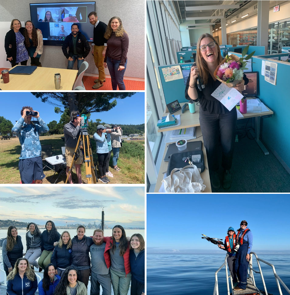
Clockwise: New Dr. Dawn Barlow with her committee after successfully defending her PhD dissertation; Lisa (me) celebrating after a successful PhD research review; Dawn and Leigh during a successful OPAL field day; the R/V Bell M. Shimada science team on the September cruise (Rachel is second from left in the back row); the 2022 TOPAZ/JASPER field team hard at work
This year, it felt like someone in the GEMM Lab was always either preparing for fieldwork, in the field, or completing the post-fieldwork tasks of gear maintenance and data download. This reality is not surprising given that we have five active projects that involve fieldwork, which keep us busy on the ocean. Another two successful gray whale field seasons are on the books! Our project GRANITE wrapped its 7th consecutive year of field work in Newport on October 15th, while the integrated projects TOPAZ/JASPER completed an 8th consecutive field season in Port Orford at the end of August. The GRANITE field team grew with the addition of Master’s student Kate Colson, who is co-advised by Leigh and Dr. Andrew Trites at University of British Columbia. Down south in Port Orford, Allison successfully led her first solo field season after taking over the project from me last year. But the nearshore is not the only place that captured the GEMM Lab’s attention. HALO (Holistic Assessment of Living marine resources off Oregon) completed three survey cruises in January, June, and July, which included the successful recovery and replacement of three hydrophones, providing Imogen and Cornell PhD student Marissa Garcia with their long-awaited acoustic data. Imogen oversees cruise coordination for this GEMM Lab effort, and several lab members have gone to sea for HALO, including Imogen, Rachel, Dawn and Leigh. We also continued our participation in the Northern California Current (NCC) cruises, where we collect marine mammal and krill data for the OPAL (Overlap Predictions About Large whales) project. Dawn, Rachel and Clara all headed out together on NOAA’s R/V Bell M. Shimada in May, while Rachel was the sole GEMM Lab representative on the September cruise. Offshore biopsy efforts and U.S. Coast Guard helicopter flights also contributed data to OPAL through the year. Finally, Leigh and Dawn also participated in the MMI-wide MOSAIC (Marine Offshore Species Assessment to Inform Clean energy) cruises in August and October. Despite spending so many hours on the water, we were productive onshore too…
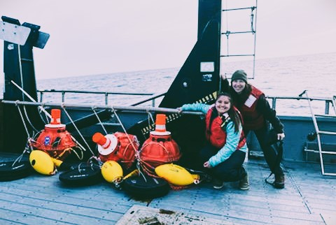
Gray whale suction cup taggingHALO hydrophones back!GRANITE field teamDawn during OPAL field workRachel, Dawn & Clara on the NCC cruise
Our faraway postdoc Solène, who has been working remotely from New Caledonia, has made steady progress on the OPAL project. Her biggest achievement this year was finishing the first, NOAA section 6-funded component, and helping to acquire funding for the second phase of the project, which Rachel started work on for her PhD. We were lucky to have Solène visit the lab in January, where she met the new and reunited with the old faces of the GEMM Lab. While her time in Oregon was only 6 weeks or so, we managed to rope her into her first and second gray whale paper (stay tuned for that sometime in 2023). And to top off our quest of making Solène an Oregonian, we are so thrilled to announce that she and her husband Micah have finally acquired their visas to move here in just a few weeks, landing in January 2023!!
Solène & Micah after receiving their visa to come to the USA in January 2023
We have been, and continue to be, busy processing and analyzing all of the rich datasets that we collect during our intense field efforts. While I do not have time to mention all of the work that occurs in the lab and on our computers, I want to highlight some of them. Our postdoctoral scholar Alejandro A. Fernández Ajó is currently back at his graduate institute, Northern Arizona University, conducting lab work to analyze the 63 fecal samples collected from 26 individual gray whales during our 2022 GRANITE field season. Rachel and her amazing team of krill interns have been doing lots of bomb calorimetry all year to better understand the caloric value of different krill species and cohorts. Imogen spent a month at Cornell University in Ithaca, New York, to hone her skills for baleen whale recognition in acoustics data and to become well acquainted with OSU affiliates Dr. Holger Klinck, PhD student Marissa Garcia, and other researchers at the K. Lisa Yang Center of Conservation Bioacoustics.
Even with all these projects underway, it seems that we cannot go a full year in the GEMM Lab without launching new endeavors. 2022 saw the creation of two more projects. For her postdoctoral research, Dawn is leading the newly-launched EMERALD (Examining Marine mammal Ecology through Region-wide Assessment of Long-term Data), which investigates spatiotemporal distribution patterns in harbor porpoise and gray whales in the nearshore NCC waters. Secondly, postdoctoral scholar KC Bierlich and Leigh have received funding to kickstart MMI’s Center of Drone Excellence (CODEX), which will launch in 2023. CODEX will focus on developing open-source tools and software to help analyze drone imagery, with the aim of offering online tutorials and hosting workshops. Both EMERALD and CODEX are funded by sales and renewals of the special Oregon gray whale license plate, which benefits MMI. We gratefully thank all the gray whale license plate holders, who made this research possible, and encourage any Oregonians that don’t have a whale on their tail yet, to do so in 2023!
Describing a year in the life of the GEMM Lab would not be complete without mentioning our outreach and education efforts as well. Allison, Clara, and I put on our teaching hats and gave guest lectures and labs for Dr. Renee Albertson and Dr. Kate Stafford’s marine mammal classes here at OSU as well as host an Introduction to R/RStudio workshop for undergraduates in our roles as coordinators for the Fisheries & Wildlife Mentorship Program. Alejandro gave a virtual talk to graduate students at the University of Pretoria South Africa about conservation physiology, highlighting his research with southern right whales. KC was invited to talk about using drones and computer science to study whales at Newport High School’s Computer Science Course and Oregon Sea Grant’s Whale Ecology Homeschool Program. He also gave the keynote presentation at the 25th Annual Salmon Bowl, part of the National Oceanic Sciences Bowl, which was hosted by OSU in February. Clara and myself were both invited speakers for Cape Perpetua’s monthly speaker series, where we presented our PhD research. Furthermore, GEMM Lab members also presented our work at numerous scientific conferences including the Society of Marine Mammal conference, Ocean Sciences, PICES annual meeting, and TWS Oregon Chapter, to name a few. The dissemination of our work to the scientific community and the public is a central focus of our lab, and we also prioritize providing hands-on opportunities and experiences to students eager to participate in ecological research. We mentored a total of 12 students in 2022, from high school to graduate level, who were involved in all aspects of our research including kayaking in Port Orford to collect prey samples, meticulously measuring drone images of whales, and spending hours hunched over microscopes identifying tiny crustaceans.
Clockwise: 2022 TOPAZ/JASPER team (Charlie, Luke, Allison, Nicola, Zoe); REU student Braden Virgil discussing his poster; krill interns Abby and Henley; REU student Celest with mentors Clara and Leigh
We have once again been prolific writers, contributing 19 total peer-reviewed publications to 15 different scientific journals. If you are in the mood for some holiday reading, you will find the full list of publications at the end of this post. All authors in bold are (or were) GEMM Lab members when the work occurred.
And YOU, our awesome, supportive readers, have once again been busy, with a whopping 25,368 views of our blog this year!!! Thank you for joining us on our 2022 journey! We hope you have enjoyed the tales that we have told and the knowledge we have (hopefully) conveyed. On one final note, if you are still looking for that perfect holiday gift for the whale-lover in your life, and if you want to support our research, consider adopting a whale from our IndividuWhale website. As a small incentive, if you adopt a whale before the end of the year, you will be entered into our Oregon South Coast Whale Watch Experience giveaway! We will reveal the giveaway winner in January 2023. We wish you all restful, happy, and most importantly, healthy holidays, and hope you will join us again in 2023!
The GEMM Lab with their white elephant gifts during our annual holiday party
Did you enjoy this blog? Want to learn more about marine life, research, and conservation? Subscribe to our blog and get a weekly message when we post a new blog. Just add your name and email into the subscribe box below.
Publications
Barlow, D.R., Klinck, H., Ponirakis, D., Holt Colberg, M., Torres, L.G. (In Press). Temporal occurrence of three blue whale populations in New Zealand waters from passive acoustic monitoring. Journal of Mammalogy.
Barlow, D.R., Estrada Jorge, M., Klinck, H., Torres, L.G. (2022). Shaken, not stirred: blue whales show no acoustic response to earthquake events. Royal Society Open Science. 9:220242.
Bierlich, K.C., Hewitt, J., Schick R.S., Pallin, L., Dale, J., Friedlaender, A.S., Christiansen, F., Sprogis K.R., Dawn, A.H., Bird, C.N., Larsen, G., Nichols, R., Shero, M., Goldbogen, J.A., Read, A., Johnston, D.W. (2022). Seasonal gain in body condition of foraging humpback whales along the Western Antarctic Peninsula. Frontiers in Marine Science. 9, 1–16. https://www.frontiersin.org/articles/10.3389/fmars.2022.1036860/full
Cade, D.E., Kahane-Rapport, S.R., Gough, W.T., Bierlich, K.C., Linksy, J.M.J., Johnston, D.W., Goldbogen, J.A., Friedlaender, A.S. (in press). Ultra-high feeding rates of Antarctic minke whales imply a lower limit for body size in engulfment filtration feeders. Nature Ecology and Evolution.
D’Agostino, V.C., Fernández Ajó, A., Degrati, M. et al. Potential endocrine correlation with exposure to domoic acid in Southern Right Whale (Eubalaena australis) at the Península Valdés breeding ground. Oecologia 198, 21–34 (2022). https://doi.org/10.1007/s00442-021-05078-4
Derville, S., Barlow, D.R., Hayslip, C., Torres, L.G. (2022). Seasonal, annual, and decadal shifts of three baleen whale species relative to dynamic ocean conditions off Oregon, USA. Frontiers in Marine Science 9:868566.
Goetz, K.T., Stephenson, F., Hoskins, A., Bindoff, A.D., Orben, R.A., Sagar, P.M., Torres, L.G., et al. (2022). Data quality influences the predicted distribution and habitat of four southern-hemisphere Albatross species. Frontiers in Marine Science 9:782923. https://doi:10.3389/fmars.2022.782923
Gough, W.T., Cade, D.E., Czapanskiy, M.F., Potvin, J., Fish, F.E, Kahane-Rapport, S.R., Savoca, M.S., Bierlich, K.C., Johnston, D.W., Friedlaender, A.S., Szabo, A., Bejder, L., Goldbogen, J.A., (2022). Fast and Furious: Energetic tradeoffs and scaling of high-speed foraging in rorqual whales. Integrative Organismal Biology, 4(1) obac038, https://doi.org/10.1093/iob/obac038
Green, C-P., Ratcliffe, N., Mattern, T., …, Torres, L.G., Hindell, M.A. (2022). The role of allochrony in influencing interspecific differences in foraging distribution during the non-breeding season between two congeneric crested penguin species. PLoS ONE https://doi.org/10.1371/journal.pone.0262901
Hildebrand, L., Sullivan, F.A., Orben, R.A., Derville, S., Torres, L.G. (2022). Trade-offs in prey quantity and quality in gray whale foraging. Marine Ecology Progress Series 695:189-201. https://doi.org/10.3354/meps14115
Hunt, K.E., Buck, C.L., Ferguson, S.H., Fernández Ajó, A., Heide-Jørgensen, M.P., Matthews, C.J.D. (2002). Male Bowhead Whale Reproductive Histories Inferred from Baleen Testosterone and Stable Isotopes, Integrative Organismal Biology, 4: obac014, https://doi.org/10.1093/iob/obac014
Lemos, L.S., Haxel, J.H., Olsen, A., Burnett, J.D., Smith, A., Chandler, T.E., Nieukirk, S.L., Larson, S.E., Hunt, K.E., Torres, L.G. (2022). Effects of vessel traffic and ocean noise on gray whale stress hormones. Scientific Reports 12:18580.
Mouton, T.L., Stephenson, F., Torres, L.G., Rayment, W., Brough, T., McLean, M., Tonkin, J.D., Albouy, C., Leprieur, F. (2022). Spatial mismatch in diversity facets reveals contrasting protection for New Zealand’s cetacean biodiversity. Biological Conservation 267:109484. https://doi.org/10.1016/j.biocon.2022.109484
Nazario, E.C., Cade, D.E., Bierlich, K.C., Czapanskiy, M.F., Goldbogen, J.A., Kahane-Rapport, S.R., van der Hoop, J.M., San Luis, M.T., Friedlaender, A.S. (2022). Baleen whale inhalation variability revealed using animal-borne video tags. PeerJ 10:e13724 https://doi.org/10.7717/peerj.13724
Pallin, L., Bierlich, K.C., Durban, J. Fearnbach, H., Savenko, O., C.S. Baker, E. Bell, Double, M.C., de la Mare, W., Goldbogen, J., Johnston, D., Kellar, N., Nichols, R., Nowacek, D., Read, A.J., Steel, D., Friedlaender, A. (2022) Demography of an ice-obligate mysticete in a region of rapid environmental change. Royal Society of Open Science. 9(11). https://doi.org/10.1098/rsos.220724
Reisinger, R.R., Brooks, C.M., Raymond, B., …, Torres, L.G., et al. (2022). Predator-derived bioregions in the Southern Ocean: Characteristics, drivers and representation in marine protected areas. Biological Conservation 272:109630. https://doi.org/10.1016/j.biocon.2022.109630
Rivers, J.W., Guerrero J.B., Brodeur, R.D., …, Torres. L.G., Barth, J.A. (2022). Critical research needs for forage fish within inner shelf marine ecosystems. Fisheries 47(5):213-221. https://doi.org/10.1002/fsh.10725
Dr. KC Bierlich, Postdoctoral Scholar, OSU Department of Fisheries, Wildlife, & Conservation Sciences, Geospatial Ecology of Marine Megafauna (GEMM) Lab
Traveling across oceans takes a lot of energy. Most baleen whales use stored energy acquired on their summer foraging grounds to support the costs of migration to and reproduction on their winter breeding grounds. Since little, if any, feeding takes place during the migration and winter season, it is essential that baleen whales obtain enough food to increase their fat reserves to support reproduction. As such, baleen whales are voracious feeders, and they typically depart the foraging grounds much fatter than when they had arrived.
So, how fat do baleen whales typically get by the end of the foraging season, and how does this differ across reproductive classes, such as a juvenile female vs. a pregnant female? Understanding these questions is key for identifying what a typical “healthy” whale looks like, information which can then help scientists and managers monitor potential impacts from environmental and anthropogenic stressors. In this blog, I will discuss a recent publication in Frontiers in Marine Science (https://doi.org/10.3389/fmars.2022.1036860) that is from my PhD dissertation with the Duke University Marine Robotics and Remote Sensing (MaRRS) Lab, and also includes GEMM lab members Allison Dawn and Clara Bird. In this study, we analyzed how humpback whales (Megaptera novaeangliae) along the Western Antarctic Peninsula (WAP) increase their fat reserves throughout the austral summer foraging season (Bierlich et al., 2022). This work also helps provide insight to the GEMM Lab’s GRANITE project (Gray whale Response to Ambient Noise Informed by Technology and Ecology), where we are interested in how Pacific Coast Feeding Group (PCFG) gray whales increase their energy reserves in response to environmental variability and increasing human activities.
Eastern South Pacific humpback whales, identified as Stock G by the International Whaling Commission, travel over 16,000 km between summer foraging grounds along the WAP and winter breeding grounds between Ecuador and Costa Rica (Fig. 1). Like most baleen whales, Stock G humpback whales were heavily exploited by 20th century commercial whaling. Recent evidence suggests that this population is recovering, with an estimated increase in population size of ~7,000 individuals in 2000 to ~19,107 in 2020 (Johannessen et al., 2022).
However, there are long-term concerns for this population. The WAP is one of the fastest warming regions on the planet, and regional populations of krill, an important food source for humpback whales, have declined steeply over the past half-century. Additionally, the WAP has seen a rapid expansion of human activities, such as tourism and krill fishing. Specifically, the WAP has experienced an increase in tourism from a total of 6,700 visitors from 59 voyages in 1990 to 73,000 visitors from 408 voyages in 2020, which may be causing increased stress levels amongst Stock G (Pallin et al., 2022). Furthermore, the krill fishery has increased harvest activities in key foraging areas for humpback whales (Reisinger et al., 2022). Understanding how humpback whales increase their energy reserves over the course of the foraging season can help researchers establish a baseline to monitor future impacts from climate change and human activities. This work also provides an opportunity for comparisons to other baleen whale populations that are also exposed to multiple stressors, such as the PCFG gray whales off the Newport Coast who are constantly exposed to vessel traffic and at risk of entanglement from fishing gear.
Figure 1. The migration route of the Stock G humpback whale population. Figure adapted from Whales of the Antarctic Peninsula Report, WWF 2018.
To understand how humpback whales increase their energy reserves throughout the foraging season, we collected drone imagery of whales along the WAP between November and June, 2017-2019 (Fig. 2). We used these images to measure the length and width of the whale to estimate body condition, which represents an animal’s relative energy reserve and can reflect foraging success (see previous blog). We collected drone imagery from a combination of research stations (Palmer Station), research vessels (Laurence M. Gould), and tour ships (One Ocean Expeditions). We used several different drones types and accounted for measurement uncertainty associated with the camera, focal length lens, altitude, and altimeter (barometer/LiDAR) from each drone (see previous blog and Bierlich et al., 2021a, 2021b). We also took biopsy samples to identify the sex of each individual and to determine if females were pregnant or not.
Figure 2. Two humpbacks gracefully swimming in the chilly water along the Western Antarctic Peninsula. Photo taken by KC Bierlich & the Duke University Marine Robotics and Remote Sensing (MaRRS) Lab.
Our final dataset included body condition measurements for 228 total individuals. We found that body condition increased linearly between November and June for each reproductive class, which included calves, juvenile females, juvenile whales of unknown sex, lactating females, mature whales of unknown sex, and non-pregnant females (Fig. 3). This was an interesting finding because a recent publication analyzing tagged whales from the same population found that humpback whales have high foraging rates in early season that then significantly decrease by February and March (Nichols et al., 2022). So, despite these reduced foraging rates throughout the season, humpback whales continue to gain substantial mass into the late season. This continued increase in body condition implies a change in krill abundance and/or quality into the late season, which may compensate for the lower feeding rates. For example, krill density and biomass increases by over an order of magnitude across the season (Reiss et al., 2017) and their lipid content increases by ~4x (Hagen et al., 1996). Thus, humpback whales likely compensate for their lower feeding rates by feeding on denser and higher quality krill, ultimately increasing their efficiency in energy deposition.
Figure 3. Body condition, here measured as Body Area Index (BAI), increases linearly for each reproductive class across the austral summer foraging season (Nov – June) for humpback whales along the Western Antarctic Peninsula. The shading represents the uncertainty around the estimated relationship. The colors represent the month of data collection.
We found that body condition increase varied amongst reproductive classes. For example, lactating females had the poorest measures of body condition across the season, reflecting the high energetic demands of nursing their calves (Fig. 3). Conversely, non-pregnant females had the highest body condition at the start of the season compared to all the other classes, likely reflecting the energy saved and recovered by skipping breeding that year. Calves, juvenile whales, and mature whales all reached similar levels of body condition by the end of the season, though mature whales will likely invest most of their energy stores toward reproduction, whereas calves and juveniles likely invest toward growth. We also found a positive relationship between the total length of lactating females and their calves, suggesting that bigger moms have bigger calves (Fig. 4). A similar trend has also been observed in other baleen whale species including southern and North Atlantic right whales (Christiansen et al., 2018; Stewart et al., 2022).
Figure 4. Big mothers have big calves. Total length (TL) measurement between mother-calf pairs. The bars around each point represents the uncertainty (95% highest posterior density intervals). The colors represent the month of data collection. The blue line represents the best fit from a Deming regression, which incorporate measurement uncertainty in both the independent (mother’s TL) and dependent variable (calf’s TL).
The results from the humpback study provide insight for my current work exploring how PCFG gray whales increase their energy reserves in relation to environmental variability and increasing human activities. Over the past seven years, the GEMM Lab has been collecting drone images of PCFG gray whales off the coast of Oregon to measure their body condition (see this GRANITE Project blog). Many of the individuals we encounter are seen across years and throughout the foraging season, providing an opportunity to evaluate how an individual’s body condition is influenced by environmental variation, stress levels, maturity, and reproduction. For example, we had nine total body condition measurements of a female PCFG whale named “Sole”, who had a curvilinear increase in body condition throughout the summer foraging season – a rapid increase in early season that slowed as the season progressed (Fig. 5). This raises many questions for us: is this how most PCFG whales typically increase their body condition during the summer? Is this increase different for pregnant or lactating females? How is this increase impacted by environmental variability or anthropogenic stressors? Repeated measurements of individuals, in addition to Sole, in different reproductive classes across different years will help us determine what body condition is considered a healthy range for gray whales. This is particularly important for monitoring any potential health consequences from anthropogenic stressors, such as vessel noise and traffic (see recent blog by GEMM Lab alum Leila Lemos). We are currently analyzing body condition measurements between 2016 – 2022, so stay tuned for upcoming results!
Figure 6. Body condition, here measured as Body Area Index (BAI), increases curvilinearly for “Sole”, a mature female Pacific Coat Feeding Group gray whale, imaged nine times along the Oregon coast in 2021. The colors represent the month of data collection.
References
Bierlich, K. C., Hewitt, J., Bird, C. N., Schick, R. S., Friedlaender, A., Torres, L. G., et al. (2021a). Comparing Uncertainty Associated With 1-, 2-, and 3D Aerial Photogrammetry-Based Body Condition Measurements of Baleen Whales. Front. Mar. Sci. 8, 1–16. doi:10.3389/fmars.2021.749943.
Bierlich, K. C., Hewitt, J., Schick, R. S., Pallin, L., Dale, J., Friedlaender, A. S., et al. (2022). Seasonal gain in body condition of foraging humpback whales along the Western Antarctic Peninsula. Front. Mar. Sci. 9, 1–16. doi:10.3389/fmars.2022.1036860.
Bierlich, K., Schick, R., Hewitt, J., Dale, J., Goldbogen, J., Friedlaender, A., et al. (2021b). Bayesian approach for predicting photogrammetric uncertainty in morphometric measurements derived from drones. Mar. Ecol. Prog. Ser. 673, 193–210. doi:10.3354/meps13814.
Christiansen, F., Vivier, F., Charlton, C., Ward, R., Amerson, A., Burnell, S., et al. (2018). Maternal body size and condition determine calf growth rates in southern right whales. Mar. Ecol. Prog. Ser. 592, 267–281.
Hagen, W., Van Vleet, E. S., and Kattner, G. (1996). Seasonal lipid storage as overwintering strategy of Antarctic krill. Mar. Ecol. Prog. Ser. 134, 85–89. doi:10.3354/meps134085.
Johannessen, J. E. D., Biuw, M., Lindstrøm, U., Ollus, V. M. S., Martín López, L. M., Gkikopoulou, K. C., et al. (2022). Intra-season variations in distribution and abundance of humpback whales in the West Antarctic Peninsula using cruise vessels as opportunistic platforms. Ecol. Evol. 12, 1–13. doi:10.1002/ece3.8571.
Nichols, R., Cade, D. E., Kahane-Rapport, S., Goldbogen, J., Simpert, A., Nowacek, D., et al. (2022). Intra-seasonal variation in feeding rates and diel foraging behavior in a seasonally fasting mammal, the humpback whale. Open Sci. 9, 211674.
Pallin, L. J., Botero-Acosta, N., Steel, D., Baker, C. S., Casey, C., Costa, D. P., et al. (2022). Variation in blubber cortisol levels in a recovering humpback whale population inhabiting a rapidly changing environment. Sci. Rep. 12, 1–13. doi:10.1038/s41598-022-24704-6.
Reisinger, R., Trathan, P. N., Johnson, C. M., Joyce, T. W., Durban, J. W., Pitman, R. L., et al. (2022). Spatiotemporal overlap of baleen whales and krill fisheries in the Antarctic Peninsula region. Front. Mar. Sci. doi:doi: 10.3389/fmars.2022.914726.
Reiss, C. S., Cossio, A., Santora, J. A., Dietrich, K. S., Murray, A., Greg Mitchell, B., et al. (2017). Overwinter habitat selection by Antarctic krill under varying sea-ice conditions: Implications for top predators and fishery management. Mar. Ecol. Prog. Ser. 568, 1–16. doi:10.3354/meps12099.
Stewart, J. D., Durban, J. W., Europe, H., Fearnbach, H., Hamilton, P. K., Knowlton, A. R., et al. (2022). Larger females have more calves : influence of maternal body length on fecundity in North Atlantic right whales. Mar. Ecol. Prog. Ser. 689, 179–189. doi:10.3354/meps14040.
After my graduation, since I have tropical blood running in my veins, I literally crossed the entire country in search of blue and sunny skies, warm weather and ocean, and of course different opportunities to continue doing research involving stressors and physiological responses in marine mammals and other marine organisms. It didn’t take me long to start a position as a postdoctoral associate with the Institute of Environment at Florida International University. I have learned so much in these past two years while mainly working with toxicology and stress biomarkers in a wide range of marine individuals including corals, oysters, fish, dolphins, and now manatees. I have started a new chapter in my life, and I am very eager to see where it takes me.
Talking about chapters… my Ph.D. thesis comprised four different chapters and I had published only the first one when I left Oregon: “Intra- and inter-annual variation in gray whale body condition on a foraging ground”. In this study we used drone-based photogrammetry to measure and compare gray whale body condition along the Oregon coast over three consecutive foraging seasons (June to October, 2016-2018). We described variations across the different demographic units, improved body condition with the progression of feeding seasons, and variations across years, with a better condition in 2016 compared to the following two years. Then in 2020, I was able to publish my second chapter entitled “Assessment of fecal steroid and thyroid hormone metabolites in eastern North Pacific gray whales”. In this study, we used gray whale fecal samples to validate and quantify four different hormone metabolite concentrations (progestins, androgens, glucocorticoids, and thyroid hormone). We reported variation in progestins and androgens by demographic unit and by year. Almost a year later, my third chapter “Stressed and slim or relaxed and chubby? A simultaneous assessment of gray whale body condition and hormone variability” was published. In this chapter, we documented a negative correlation between body condition and glucocorticoids, meaning that slim whales were more stressed than the chubby ones.
These three chapters were “relatively easy” to publish compared to my fourth chapter, which had a long and somewhat stressful process (which is funny as I am trying to report stress responses in gray whales). Changes between journals, titles, analyses, content, and focus had to be made over the past year and a half for it to be accepted for publication. However, I believe that it was worth the extra work and invested time as our research definitely became more robust after all of the feedback provided by the reviewers. This chapter, now entitled “Effects of vessel traffic and ocean noise on gray whale stress hormones” was finally published earlier this month at the Nature Scientific Reports journal, and I’ll describe it further below.
Increased human activities in the last decades have altered the marine ecosystem, leaving us with a noisier, warmer, and more contaminated ocean. The noise caused by the dramatic increase in commercial and recreational shipping and vessel traffic1-3 has been associated with negative impacts on marine wildlife populations4,5. This is especially true for baleen whales, whose frequencies primarily used for communication, navigation, and foraging6,7 are “masked” by the noise generated by this watercraft. Several studies have reported alterations in marine mammal behavioral states8-11, increased group cohesion12-14, and displacement8,15 due to this disturbance, however, just a few studies have considered their physiological responses. Examples of physiological responses reported in marine mammals include altered metabolic rate15,16 and variations in stress-related hormone (i.e., glucocorticoids) concentrations relative to vessel abundance and ambient noise17,18. Based on this context and on the scarcity of such assessments, we attempted to determine the effects of vessel traffic and associated ambient noise, as well as potential confounding variables (i.e., body condition, age, sex, time), on gray whale fecal glucocorticoid concentrations.
In addition to the data used in my previous three chapters collected from gray whales foraging off the Oregon coast, we also collected ambient noise levels using hydrophones, vessel count data from the Oregon Department of Fish and Wildlife (ODFW), and wind data from NOAA National Data Buoy Center (NDBC). Our first finding was a positive correlation between vessel counts and underwater noise levels (Fig. 1A), likely indicating that vessel traffic is the dominant source of noise in the area. To confirm this, we also compared underwater noise levels with wind speed (Fig. 1B), but no correlations were found.
Figure 1: Linear correlations between noise levels (daily median root mean square [rms] sound pressure level [SPL] in dB [re 1 μPa]; 50–1000 Hz) recorded on a hydrophone deployed outside the Newport harbor entrance during June to October of 2017 and 2018 and (A) vessel counts in Newport and Depoe Bay, Oregon, USA, and (B) daily median wind speed (m/s) from an anemometer station located on South Beach, Newport, Oregon, USA (station NWPO3). Asterisk indicates significant correlations between SPL and vessel counts in both years.
We also investigated noise levels by the hour of the day (Fig. 2), and we found that noise levels peaked between 6 and 8 am most days, coinciding with the peak of vessels leaving the harbor to get to fishing grounds. Another smaller peak is seen at 12 pm, which may represent “half-day fishing charter” vessels returning to the harbor. In contrast, wind speeds (in the lower graph) peaked between 3 and 4 pm, thus confirming the absence of correlation between noise and wind and providing more evidence that noise levels are dominated by the vessel activity in the area.
Figure 2: Median noise levels (root mean square sound pressure levels—SPLrms) for each hour of each day recorded on a hydrophone (50–10,000 Hz) deployed outside the Newport harbor entrance during June to October of 2017 (middle plot) and 2018 (upper plot), and hourly median noise level (SPL) against hourly median wind speed (lower plot) from an anemometer station located on South Beach, Newport, Oregon, USA (station NWPO3) over the same time period.
Finally, we assessed the effects of vessel counts, month, year, sex, whale body condition, and other hormone metabolites on glucocorticoid metabolite (GCm; “stress”) concentrations. Since we are working with fecal samples, we needed to consider the whale gut transit time and go back in time to link time of exposure (vessel counts) to response (glucocorticoid concentrations). However, due to uncertainty regarding gut transit time in baleen whales, we compared different time lags between vessel counts and fecal collection. The gut transit time in large mammals is ~12 hours to 4 days3,19,20, so we investigated the influence of vessel counts on whale “stress hormone levels” from the previous 1 to 7 days. The model with the most influential temporal scale included vessel counts from previous day, which showed a significant positive relationship with GCm (the “stress hormone level”) (Fig. 3).
Figure 3: The effect of vessel counts in Newport and Depoe Bay (Oregon, USA) on the day before fecal sample collection on gray whale fecal glucocorticoid metabolite (GCm) concentrations.
Thus, the “take home messages” of our study are:
The soundscape in our study area is dominated by vessel noise.
Vessel counts are strongly correlated with ambient noise levels in our study area.
Gray whale glucocorticoid levels are positively correlated with vessel counts from previous day meaning that gray whale gut transit time may occur within ~ 24 hours of the disturbance event.
These four chapters were all very important studies not only to advance the knowledge of gray whale and overall baleen whale physiology (as this group is one of the most poorly understood of all mammals given the difficulties in sample collection21), but also to investigate potential sources for the unusual mortality event that is currently happening (2019-present) to the Eastern North Pacific population of gray whales. Such studies can be used to guide future research and to inform population management and conservation efforts regarding minimizing the impact of anthropogenic stressors on whales.
I am very glad to be part of this project, to see such great fruits from our gray whale research, and to know that this project is still at full steam. The GEMM Lab continues to collect and analyze data for determining gray whale body condition and physiological responses in association with ambient noise (Granite, Amber and Diamond projects). The gray whales thank you for this!
Cited Literature
1. McDonald, M. A., Hildebrand, J. A. & Wiggins, S. M. Increases in deep ocean ambient noise in the Northeast Pacific west of San Nicolas Island, California. J. Acoust. Soc. Am. 120, 711–718 (2006).
2. Kaplan, M. B. & Solomon, S. A coming boom in commercial shipping? The potential for rapid growth of noise from commercial ships by 2030. Mar. Policy 73, 119–121 (2016).
3. McCarthy, E. International regulation of underwater sound: establishing rules and standards to address ocean noise pollution (Kluwer Academic Publishers, 2004).
4. Weilgart, L. S. The impacts of anthropogenic ocean noise on cetaceans and implications for management. Can. J. Zool. 85, 1091–1116 (2007).
5. Bas, A. A. et al. Marine vessels alter the behaviour of bottlenose dolphins Tursiops truncatus in the Istanbul Strait, Turkey. Endanger. Species Res. 34, 1–14 (2017).
6. Erbe, C., Reichmuth, C., Cunningham, K., Lucke, K. & Dooling, R. Communication masking in marine mammals: a review and research strategy. Mar. Pollut. Bull. 103, 15–38 (2016).
7. Erbe, C. et al. The effects of ship noise on marine mammals: a review. Front. Mar. Sci. 6 (2019).
8. Sullivan, F. A. & Torres, L. G. Assessment of vessel disturbance to gray whales to inform sustainable ecotourism. J. Wildl. Manag. 82, 896–905 (2018).
9. Pirotta, E., Merchant, N. D., Thompson, P. M., Barton, T. R. & Lusseau, D. Quantifying the effect of boat disturbance on bottlenose dolphin foraging activity. Biol. Conserv. 181, 82–89 (2015).
10. Dans, S. L., Degrati, M., Pedraza, S. N. & Crespo, E. A. Effects of tour boats on dolphin activity examined with sensitivity analysis of Markov chains. Conserv. Biol. 26, 708–716 (2012).
11. Christiansen, F., Rasmussen, M. & Lusseau, D. Whale watching disrupts feeding activities of minke whales on a feeding ground. Mar. Ecol. Prog. Ser. 478, 239–251 (2013).
12. Bejder, L., Samuels, A., Whitehead, H. & Gales, N. Interpreting short-term behavioural responses to disturbance within a longitudinal perspective. Anim. Behav. 72, 1149–1158 (2006).
13. Nowacek, S. M., Wells, R. S. & Solow, A. R. Short-term effects of boat traffic on Bottlenose dolphins, Tursiops truncatus, in Sarasota Bay, Florida. Mar. Mammal. Sci. 17, 673–688 (2001).
14. Bejder, L., Dawson, S. M. & Harraway, J. A. Responses by Hector’s dolphins to boats and swimmers in Porpoise Bay, New Zealand. Mar. Mammal Sci. 15, 738–750 (1999).
15. Lusseau, D. Male and female bottlenose dolphins Tursiops spp. have different strategies to avoid interactions with tour boats in Doubtful Sound. New Zealand. Mar. Ecol. Prog. Ser. 257, 267–274 (2003).
16. Sprogis, K. R., Videsen, S. & Madsen, P. T. Vessel noise levels drive behavioural responses of humpback whales with implications for whale-watching. Elife 9, e56760 (2020).
17. Ayres, K. L. et al. Distinguishing the impacts of inadequate prey and vessel traffic on an endangered killer whale (Orcinus orca) population. PLoS ONE 7, e36842 (2012).
18. Rolland, R. M. et al. Evidence that ship noise increases stress in right whales. Proc. R. Soc. B Biol. Sci. 279, 2363–2368 (2012).
19. Wasser, S. K. et al. A generalized fecal glucocorticoid assay for use in a diverse array of nondomestic mammalian and avian species. Gen. Comp. Endocrinol. 120, 260–275 (2000).
20. Hunt, K. E., Trites, A. W. & Wasser, S. K. Validation of a fecal glucocorticoid assay for Steller sea lions (Eumetopias jubatus). Physiol. Behav. 80, 595–601 (2004).
21. Hunt, K. E. et al. Overcoming the challenges of studying conservation physiology in large whales: a review of available methods. Conserv. Physiol. 1, cot006–cot006 (2013).
Dr. Alejandro A. Fernández Ajó, Postdoctoral Scholar, Marine Mammal Institute – OSU Department of Fisheries, Wildlife, & Conservation Sciences, Geospatial Ecology of Marine Megafauna (GEMM) Lab.
The English language is recognized as the international language of science (Gordin, 2015); I believe this is a useful convention that allows scientists to communicate ideas and gain access to global scientific literature regardless of their origin or native tongue. However, this avenue for sharing knowledge is open only for those proficient in English, and many scientists and users of scientific information, such as policy makers and conservationists, communicate on a daily basis in languages other than English. This inevitably creates barriers to the transfer of knowledge between communities, potentially impacting conservation and management because scientific knowledge is often unavailable in local languages.
Although in non-English speaking countries, local journals are receptive to publishing scientific research in languages other than English (i.e., their local language), oftentimes these local journals are perceived as low-quality and have a relatively low impact factor, making publishing in such journals less attractive to scientists. Therefore, readers with language barriers only have access to limited studies and are often unaware of the most significant research, even when the research is conducted in their region. This situation can result in a void of information relevant for environmental policies and conservation strategies. Ensuring that research findings are available in the local language of the region in which the research is conducted is an important step in science communication, but one that is often neglected.
In addition, scientists with English as a Foreign Language (EFL) confront the added challenge of navigating a second language while writing manuscripts, preparing and presenting oral presentations, and developing outreach communications (Ramirez-Castaneda, 2020). For example, EFL researchers have reported that one of the primary targets of criticism for their manuscripts under review is often the quality of their English rather than the science itself (Drubin and Kellogg, 2012). In academia, most job interviews and PhD applications are conducted in English; and grant and project proposals are often required to be written in English, which can be particularly challenging and can impact the allocation of resources for research and conservation in non-English speaking regions.
I am from Argentina, and I am a native Spanish speaker. I am fortunate to have started learning English at an early age and continue practicing with international collaborations and traveling abroad. Being able to communicate in English has opened many doors for me, but I recognize that I am in a privileged position with respect to many Argentinians and South Americans in general, where the majority of the population receives minimal training in English and bilingualism with English is very low. Thus, socioeconomic status can influence English proficiency, which then determines scientific success and access to knowledge. I believe that the scientific community should be aware of these issues and work towards improving equality in the process of research collaborations. Providing opportunities for students, and enhancing the availability of scientific knowledge for non-English speaking communities, particularly when the research is relevant for such communities.
In this picture I am with an international group of Fulbright scholars during the Spring International Language Program at the University of Arkansas. This is on of many activities organized by the Fulbright program to create bridges across cultures and languages.
Fortunately, there are several examples pointing towards improving equality in the scientific process, access to knowledge, and opportunities for EFL communities in STEM careers. Several journals are now accepting, or considering to accept the publication of papers in multiple languages. One example of this is the journal Integrative Organismal Biology, which provides the option for publishing the paper abstract in multiple languages. In our recent publication, “Male Bowhead Whale Reproductive Histories Inferred from Baleen Testosterone and Stable Isotopes,” we provided an abstract in five different languages, including Inuktitut, one of primary languages of indigenous groups in the area. And, international exchange programs like the Fulbright Foreign Student Program, of which I was a beneficiary between 2018-2020, enable graduate students and young professionals from abroad to study and conduct research in the United States.
In an effort to contribute to addressing these problems, I am working with a group of colleagues from Argentina (María Constanza (Kata) Marchesi and Tomas Marina) to develop graduate level coursework that will be offered at the Universidad Nacional de la Patagonia in Puerto Madryn, Argentina, with the objective to enable students to learn effective communication using English in the scientific environment. Unfortunately, these types of programs focused on EFL proficiency for STEM students are currently rare in Argentina, but my hope is that our work can spur the creation of additional programs for EFL students in STEM across the region.
I want to finish this post with the acknowledgement of the huge support I have form the GEMM Lab, which welcomes diversity, equity, and inclusivity, and promotes a culture of anti-racism, transparency, and acceptance (See the GEMM Lab DEI statement here).
Did you enjoy this blog? Want to learn more about marine life, research and conservation? Subscribe to our blog and get weekly updates and more! Just add your name into the subscribe box below!
References and Additional Readings
Gordin, M. D. (2015). Scientific Babel : How Science Was Done Before and After Global English. Chicago, IL: University of Chicago Press.
Ramírez-Castañeda V (2020) Disadvantages in preparing and publishing scientific papers caused by the dominance of the English language in science: The case of Colombian researchers in biological sciences. PLoS ONE 15(9): e0238372. https://doi.org/10.1371/journal.pone.0238372
Drubin, D. G., and Kellogg, D. R. (2012). English as the universal language of science: opportunities and challenges. Mol. Biol. Cell 23:1399. doi: 10.1091/mbc.E12-02-0108
Amano, T., González-Varo, J. P., & Sutherland, W. J. (2016). Languages are still a major barrier to global science. PLoS Biology, 14(12), e2000933. https://doi.org/10.1371/journal.pbio.2000933
Marden, E., Abbott, R. J., Austerlitz, F., Ortiz-Barrientos, D., Rieseberg, L. H. (2021). Sharing and reporting benefits from biodiversity research. Molecular Ecology, 30(5), 1103–1107. https://doi.org/10.1111/mec.15702
Márquez, M. C., & Porras, A. M. (2020). Science communication in multiple languages Is critical to Its effectiveness. Frontiers in Communication, 5(May). https://doi.org/10.3389/fcomm.2020.00031
Ramírez-Castañeda V (2020) Disadvantages in preparing and publishing scientific papers caused by the dominance of the English language in science: The case of Colombian researchers in biological sciences. PLoS ONE 15(9): e0238372. https://doi.org/10.1371/journal.pone.0238372
Trisos, C. H., Auerbach, J., & Katti, M. (2021). Decoloniality and anti-oppressive practices for a more ethical ecology. Nature Ecology and Evolution, 5(9), 1205–1212. https://doi.org/10.1038/s41559-021-01460-w
Letter to the Editor of Marine Mammal Science: Enhancing the impact and inclusivity of research by embracing multi-lingual science communication (2022) DOI: 10.13140/RG.2.2.29934.08001 http://dx.doi.org/10.13140/RG.2.2.29934.08001
Leal, J. S., Soares, B., Franco, A. C. S., de Sá Ferreira Lima, R. G., Baker, K., & Griffiths, M. (2022). Decolonizing ecological research: a debate between global North geographers and global South field ecologists. https://doi.org/10.31235/osf.io/wbzh2