Making predictions: A window into ecological forecast models

By Dawn Barlow, PhD Candidate, OSU Department of Fisheries, Wildlife and Conservation Sciences, Geospatial Ecology of Marine Megafauna Lab

“What is the weather going to be like tomorrow?” “How long will it take to drive there, with traffic?” We all rely on forecasts to make decisions, such as whether to bring a rain jacket, when to get in the car to arrive at a certain destination on time, or any number of situations where we want a prediction of what will happen in the near future. Statistical models underpin many of these examples, using past data to inform future predictions.

Early on in graduate school, I was told that “all models are wrong, but some models work.” Any model is essentially a best approximation, using mathematical relationships, of how we understand a pattern. Models are powerful tools in ecology, enabling us to distill complex, dynamic, and interacting systems into terms and parameters that can be quantified. This ability can help us better understand our study systems and use that understanding to make predictions. We will never be able to describe every nuance of an ecosystem. Instead, the challenge is to collect enough information to build an informed model that can enhance our understanding, without over-simplifying or unnecessarily complicating the system we aim to describe. As Dr. Simon Levin stated in his 1989 seminal paper:

A good model does not attempt to reproduce every detail of the biological system; the system itself suffices for that purpose as the most detailed model of itself. Rather, the objective of a model should be to ask how much detail can be ignored without producing results that contradict specific sets of observations, on particular scales of interest.”1

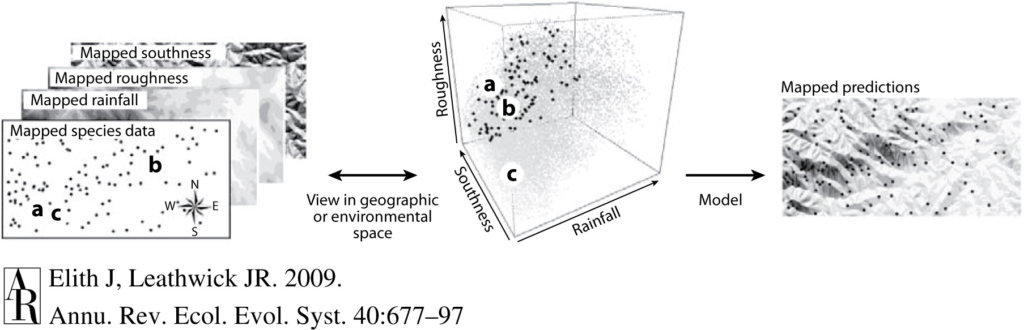
Species distribution models (SDMs) are the particular branch of models that underpin much of my PhD research on blue whale ecology and distribution in New Zealand. SDMs are mathematical algorithms that correlate observations of a species with environmental conditions at their observed locations to gain ecological insight and predict spatial distributions of the species (Fig. 1)2. The model is a best attempt to quantify and describe the relationships between predictors, e.g., temperature and the observed species distribution pattern. For example, blue whale occurrence is higher in areas of lower temperatures and greater krill availability, and these relationships can be described with models3. So, a model essentially takes all the data available, and synthesizes that information in terms of the relationships between the predictors (environment) and response (species occurrence). Then, we can look at the fitted relationships to ask what we would expect from the species distribution pattern when temperature, or krill availability, or any other predictor, is at a particular value. 

Figure 1. A schematic of a species distribution model (SDM) illustrating how the relationship between mapped species and environmental data (left) is compared to describe “environmental space” (center), and then map predictions from a model using only environmental predictors (right). Note that inter-site distances in geographic space might be quite different from those in environmental space—a and c are close geographically, but not environmentally. The patterning in the predictions reflects the spatial autocorrelation of the environmental predictors. Figure reproduced from Elith and Leathwick (2009).

So, if a model is simply a mathematical description of how terms interact to produce a particular outcome, how do predictions work? To make a spatial prediction, e.g., a map of the probability of a species being present, you need two things: a model describing the functional relationships between species presence and your environmental predictors, and the values of your predictor variables on the day you are interested in predicting to. For example, you may need to obtain a map of sea surface temperature, productivity, temperature anomaly, and surface currents on a day you want to know where whales are expected to be. Your model is the applied across that stack of spatial environmental layers and, based on the functional relationships derived by the model, you get an estimate of the probability of species occurrence based on the temperature, productivity, anomaly, and surface current values at each location. By applying the model over a range of values, you can obtain a continuous surface with the probability of presence, in the form of a map. These maps are typically for the past or present because that is when we can typically acquire spatial environmental layers. However, to make predictions for a future time of interest, we need to have spatial environmental layers for the future.

Forecasts are predictions for the future. Recent advances in technology and computing have led to an emergence of environmental and ecological forecasting tools that are being developed around the world to produce marine forecasts. These tools include predictions of the physical environment such as ocean temperatures or currents, and biological patterns such as where species will be distributed in space and timing of events like salmon spawning or lobster landings4. The ability to generate forecast of marine ecosystems is of particular interest to resource users and managers because it can allow them to be proactive rather than reactive. Forecasts enable us to anticipate events or patterns and prepare, rather than having to respond in real-time or after the fact.

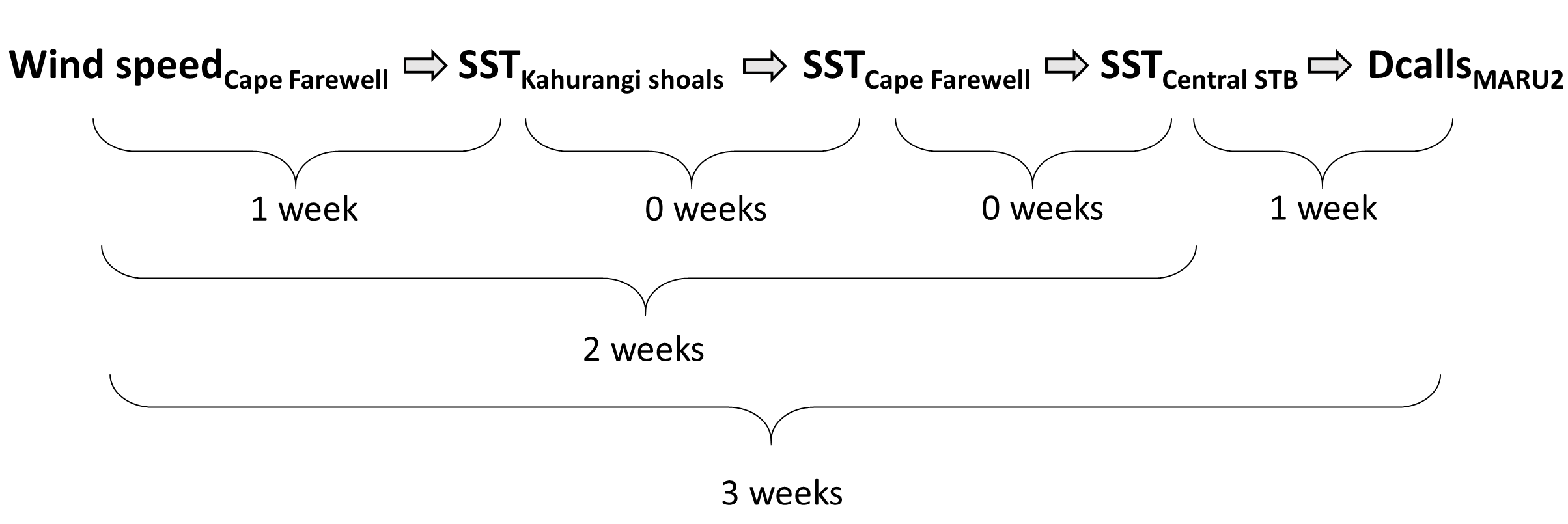
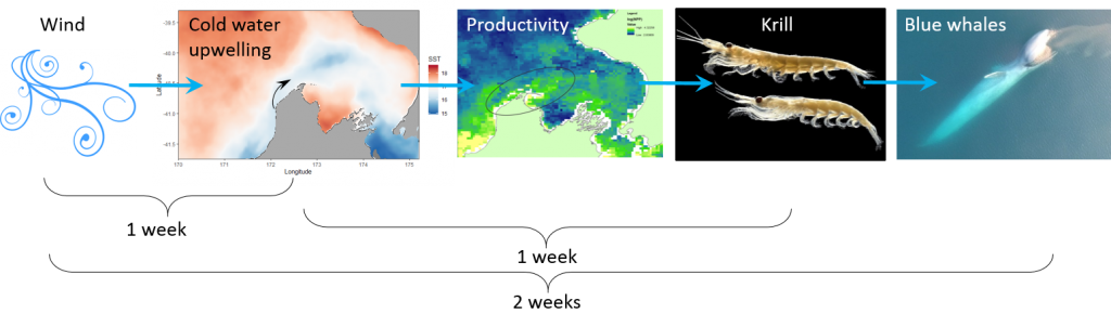
The South Taranaki Bight region in New Zealand is an area where blue whale foraging habitat frequently coincides with industry pressures, including petroleum and mineral extraction, exploration for petroleum reserves using seismic airgun surveys, vessel traffic between ports, and even an ongoing proposal for seabed mining5. Static spatial restrictions to mitigate impacts from these activities on blue whales may be met with resistance from industry user groups, but dynamic spatial management6–8 of blue whale habitat could be more attractive and acceptable. The key for successful dynamic management is knowing where and when to put those boundaries; and this is where ecological forecast models can show their strength. If we can predict suitable blue whale habitat for the future, proactive regulations can be applied to enhance conservation management in the region. Can we develop reliable and useful ecological forecasts for the South Taranaki Bight? Well, given that we have already developed robust models of the relationships between blue whales and their habitat3 and have documented the spatial and temporal lags between wind, upwelling, and blue whales9, we feel confident that we can develop forecast models to predict where blue whales will be in the STB region. As we continue working hard toward this goal, we invite you to check back for our findings in the future. So, consider this blog post a forecast of sorts, and stay tuned!  

Figure 2. A blue whale surfaces in front of an oil extraction platform in the South Taranaki Bight, demonstrating the overlap between whales and industry in the region. Photo by D. Elvines.

References:

1.        Levin, S. A. The problem of pattern and scale. Ecology 73, 1943–1967 (1992).

2.        Elith, J. & Leathwick, J. R. Species Distribution Models: Ecological Explanation and Prediction Across Space and Time. Annu. Rev. Ecol. Evol. Syst. 40, 677–697 (2009).

3.        Barlow, D. R., Bernard, K. S., Escobar-Flores, P., Palacios, D. M. & Torres, L. G. Links in the trophic chain: Modeling functional relationships between in situ oceanography, krill, and blue whale distribution under different oceanographic regimes. Mar. Ecol. Prog. Ser. 642, 207–225 (2020).

4.        Payne, M. R. et al. Lessons from the first generation of marine ecological forecast products. Front. Mar. Sci. 4, 1–15 (2017).

5.        Torres, L. G. Evidence for an unrecognised blue whale foraging ground in New Zealand. New Zeal. J. Mar. Freshw. Res. 47, 235–248 (2013).

6.        Hyrenbach, K. D., Forney, K. A. & Dayton, P. K. Marine protected areas and ocean basin management. Aquat. Conserv. Mar. Freshw. Ecosyst. 10, 437–458 (2000).

7.        Maxwell, S. M. et al. Dynamic ocean management: Defining and conceptualizing real-time management of the ocean. Mar. Policy 58, 42–50 (2015).

8.        Oestreich, W. K., Chapman, M. S. & Crowder, L. B. A comparative analysis of dynamic management in marine and terrestrial systems. Front. Ecol. Environ. 18, 496–504 (2020).

9.        Barlow, D. R., Klinck, H., Ponirakis, D., Garvey, C. & Torres, L. G. Temporal and spatial lags between wind, coastal upwelling, and blue whale occurrence. Sci. Rep. 11, (2021).

Fashionably late: New GEMM Lab publication measures lags between wind, upwelling, and blue whale occurrence

By Dawn Barlow, PhD Candidate, OSU Department of Fisheries and Wildlife, Geospatial Ecology of Marine Megafauna Lab

To understand the complex dynamics of an ecosystem, we need to examine how physical forcing drives biological response, and how organisms interact with their environment and one another. The largest animal on the planet relies on the wind. Throughout the world, blue whales feed areas where winds bring cold water to the surface and spur productivity—a process known as upwelling. In New Zealand’s South Taranaki Bight region (STB), westerly winds instigate a plume of cold, nutrient-rich waters that support aggregations of krill, and ultimately lead to foraging opportunities for blue whales. This pathway, beginning with wind input and culminating in blue whale occurrence, does not take place instantaneously, however. Along each link in this chain of events, there is some lag time.

Figure 1. A blue whale comes up for air in New Zealand’s South Taranaki Bight. Photo: L. Torres.

Our recent paper published in Scientific Reports examines the lags between wind, upwelling, and blue whale occurrence patterns. While marine ecologists have long acknowledged that lag plays a role in what drives species distribution patterns, lags are rarely measured, tested, and incorporated into studies of marine predators such as whales. Understanding lags has the potential to greatly improve our ability to predict when and where animals will be under variable environmental conditions. In our study, we used timeseries analysis to quantify lag between different metrics (wind speed, sea surface temperature, blue whale vocalizations) at different locations. While our methods are developed and implemented for the STB ecosystem, they are transferable to other upwelling systems to inform, assess, and improve predictions of marine predator distributions by incorporating lag into our understanding of dynamic marine ecosystems.

So, what did we find? It all starts with the wind. Wind instigates upwelling over an area off the northwest coast of the South Island of New Zealand called Kahurangi Shoals. This wind forcing spurs upwelling, leading to the formation of a cold water plume that propagates into the STB region, between the North and South Islands, with a lag of 1-2 weeks. Finally, we measured the density of blue whale vocalizations—sounds known as D calls, which are produced in a social context, and associated with foraging behavior—recorded at a hydrophone downstream along the upwelling plume’s path. D call density increased 3 weeks after increased wind speeds near the upwelling source. Furthermore, we looked at the lag time between wind events and aggregations in blue whale sightings. Blue whale aggregations followed wind events with a mean lag of 2.09 ± 0.43 weeks, which fits within our findings from the timeseries analysis. However, lag time between wind and whales is variable. Sometimes it takes many weeks following a wind event for an aggregation to form, other times mere days. The variability in lag can be explained by the amount of prior wind input in the system. If it has recently been windy, the water column is more likely to already be well-mixed and productive, and so whale aggregations will follow wind events with a shorter lag time than if there has been a long period without wind and the water column is stratified.

Figure 2. Top panel: Map of the study region within the South Taranaki Bight (STB) of New Zealand, with location denoted by the white rectangle on inset map in the upper right panel. All spatial sampling locations for sea surface temperature implemented in our timeseries analyses are denoted by the boxes, with the four focal boxes shown in white that represent the typical path of the upwelling plume originating off Kahurangi shoals and moving north and east into the STB. The purple triangle represents the Farewell Spit weather station where wind measurements were acquired. The location of the focal hydrophone (MARU2) where blue whale D calls were recorded is shown by the green star. (Reproduced from Barlow et al. 2021). Bottom panel: Results of the timeseries cross-correlation analyses, illustrating the lag between some of the metrics and locations examined.

This publication forms the second chapter of my PhD dissertation. However, in reality it is the culmination of a team effort. Just as whale aggregations lag wind events, publications lag years of hard work. The GEMM Lab has been studying New Zealand blue whales since Leigh first hypothesized that the STB was an undocumented foraging ground in 2013. I was fortunate enough to join the research effort in 2016, first as a Masters student and now as a PhD Candidate. I remember standing on the flying bridge of R/V Star Keys in New Zealand in 2017, when early in our field season we saw very few blue whales. Leigh and I were discussing this, with some frustration. Exclamations of “This is cold, upwelled water! Where are the whales?!” were followed by musings of “There must be a lag… It has to take some time for the whales to respond.” In summer 2019, Christina Garvey came to the GEMM Lab as an intern through the NSF Research Experience for Undergraduates program. She did an outstanding job of wrangling remote sensing and blue whale sighting data, and together we took on learning and understanding timeseries analysis to quantify lag. In a meeting with my PhD committee last spring where I presented preliminary results, Holger Klinck chimed in with “These results are interesting, but why haven’t you incorporated the acoustic data? That is a whale timeseries right there and would really add to your analysis”. Dimitri Ponirakis expertly computed the detection area of our hydrophone so we could adequately estimate the density of blue whale calls. Piecing everything together, and with advice and feedback from my PhD committee and many others, we now have a compelling and quantitative understanding of the upwelling dynamics in the STB ecosystem, and have thoroughly described the pathway from wind to whales in the region.

Figure 3. Dawn and Leigh on the flying bridge of R/V Star Keys on a windy day in New Zealand during the 2017 field season. Photo: T. Chandler.

Our findings are exciting, and perhaps even more exciting are the implications. Understanding the typical patterns that follow a wind event and how the upwelling plume propagates enables us to anticipate what will happen one, two, or up to three weeks in the future based on current conditions. These spatial and temporal lags between wind, upwelling, productivity, and blue whale foraging opportunities can be harnessed to generate informed forecasts of blue whale distribution in the region. I am thrilled to see this work in print, and equally thrilled to build on these findings to predict blue whale occurrence patterns.

Reference: Barlow, D.R., Klinck, H., Ponirakis, D., Garvey, C., Torres, L.G. Temporal and spatial lags between wind, coastal upwelling, and blue whale occurrence. Sci Rep 11, 6915 (2021). https://doi.org/10.1038/s41598-021-86403-y

New Zealand blue whale research in the time of COVID

By Grace Hancock, Undergraduate Student at Kalamazoo College MI, GEMM Lab Intern (June 2020 to present)

It feels safe to say that everyone’s plans for the summer of 2020 went through a roller coaster of changes due to the pandemic. Instead of the summer research or travel plans that many undergraduate students, including myself, expected, many of us found ourselves at home, quarantining, and unsure of what to do with our time. Although it was unexpected, all that extra time brought me serendipitously to the virtual doorstep of the GEMM Lab. A few zoom calls and many, many emails later I am now lucky to be a part of the New Zealand Blue Whale photo-ID team. Under Leigh’s and Dawn’s guidance, I picked up the photo identification project where they had left it and am helping to advance this project to its next stage.

The skin of a blue whale is covered by distinct markings similar to a unique fingerprint. Thus, these whales can have a variety of markings that we use to identify them, including mottled pigmentation, pock marks (often caused by cookie cutter sharks), blisters, and even holes in the dorsal fins and flukes.

Figure 1. Examples of skin conditions that help in matching demonstrated on a photo of NZBW052 on the 10/9/2015

True blue blog fans may remember that in 2016 Dawn began the very difficult work of creating a photo ID catalog of all the blue whales that the GEMM Lab had encountered during field work in the South Taranaki Bight in New Zealand. Since that post, the catalog has grown and become an incredibly useful tool. When I came to the lab, I received a hard drive containing all the work Dawn had done to-date with the catalog, as well as two years of photos from various whale watching trips in the Hauraki Gulf of New Zealand. The goal of my internship was to integrate these photos into the GEMM catalog Dawn had created and, hopefully, identify some matches of whales between the two datasets.  If there were any matches – and if I found no matches – we would gain information about whale movement patterns and abundance in New Zealand waters.

Before we could dive into this exciting matching work, there was lots of data organization to be done. Most of the photos I analyzed were provided by the Auckland Whale and Dolphin Safari (AWADS), an eco-tourism company that does regular whale watching trips in the Hauraki Gulf, off the North Island of New Zealand. The photos I worked with were taken by people with no connection to the lab and, because of this, were often filled with pictures of seals, birds, and whatever else caught the whale watcher’s eye. This dataset led to hours of sorting, renaming, and removing photos. Next, I evaluated each photo of a whale to determine photo-quality (focus, angle to the camera, lighting) and then I used the high-quality photos where markings are visible to begin the actual matching of the whales.

Figure 2. The fluke of NZBW013 taken on 2/2/2016 with examples of unique nicks and markings that could be used to match

Blue whales are inarguably massive organisms. For this reason, it can be hard to know what part of the whale you’re looking at. To match the photos to the catalog, I found the clearest pictures that included the whale’s dorsal fin. For each whale I tried to find a photo from the left side, the right side, and (if possible) an image of its fluke. I could then compare these photos to the ones organized in the catalog developed by Dawn.

The results from my matching work are not complete yet, but there are a few interesting tidbits that I can share with our readers today. From the photos submitted by AWADS, I was able to identify twenty-two unique individual whales. We are in the process of matching these whales to the catalog and, once this is done, we will know how many of these twenty-two are whales we have seen before and how many are new individuals. One of the most exciting matches I made so far is of a whale known in our catalog as individual NZBW072. Part of what made this whale so exciting was the fact that it is the calf of NZBW031 who was spotted eight times from 2010-2017, in the Hauraki Gulf, off Kaikoura, and in the South Taranaki Bight. As it turns out, NZBW072 took after her mother and has been spotted a shocking nine times from 2010 to 2019, all in the Hauraki Gulf region. Many of the whales in our catalog have only been spotted once, so encountering two whales with this kind of sighting track record that also happen to be related is like hitting the jackpot.

Figure 3. NZBW072 photographed on 11/8/2010 (top photo taken by Rochelle Constantine in the Hauraki Gulf) and on 10/3/2019 (bottom photo taken by the Auckland Whale and Dolphin Safari) with marks circled in red or yellow to highlight the matched features.

Once I finish comparing and matching the rest of these photos, the catalog will be substantially more up-to-date. But that is not where the work stops. More photos of blue whales in New Zealand are frequently being captured, either by whale watchers in the Hauraki Gulf, fellow researchers on the water, keen workers on oil and gas rigs, or the GEMM Lab. Furthermore, the GEMM Lab contributes these catalog photos to the International Whaling Commission (IWC) Southern Hemisphere Blue Whale Catalog, which compiles all photos of blue whales in the Southern Ocean and enables interesting and critical conservation questions to be addressed, like “How many blue whales are there in the Southern Ocean?” Once I complete the matching of these 22 individuals, I will upload and submit them to this IWC collaborative database on behalf of the GEMM Lab. This contribution will expand the global knowledge of these whales and motivates me to continue this important photo ID work. I am so excited to be a part of this effort, through which I have learned important skills like the basics of science communication (through writing this blog post) and attention to detail (from working very closely with the photos I was matching). I know both of these skills, and everything else I have learned from this process, will help me greatly as I begin my career in the next few years. I can tell big things will come from this catalog and I will forever be grateful for the chance I have had to contribute to it.

What makes a good meal for a hungry whale?

By Dawn Barlow, PhD student, OSU Department of Fisheries and Wildlife, Geospatial Ecology of Marine Megafauna Lab

In the vast and dynamic marine environment, food is notoriously patchy and ephemeral [1]. Predators such as marine mammals and seabirds must make a living in this dynamic environment by locating and capturing those prey patches. Baleen whales such as blue and humpback whales have a feeding strategy called “lunge feeding”, whereby they accelerate forward and open their massive jaws, engulf prey-laden water in their buccal pouch that expands like an accordion, and filter the water out through baleen plates so that they are left with a mouthful of food (Fig. 1) [2]. This approach is only efficient if whales can locate and target dense prey patches that compensate for the energetic costs of diving and lunging [3]. Therefore, not only do these large predators need to locate enough food to survive in the expansive and ever-changing ocean, they need to locate food that is dense enough to feed on, otherwise they actually lose more energy by lunging than they gain from the prey they engulf.

Figure 1. Schematic of a humpback whale lunge feeding on a school of fish. Illustration by Alex Boersma.

Why do baleen whales rely on such a costly feeding approach? Interestingly, this tactic emerged after the evolution of schooling behavior of prey such as zooplankton and forage fish (e.g., herring, anchovy, sand lance) [4]. Only because the prey aggregate in dense patches can these large predators take advantage of them by lunge feeding, and by engulfing a whole large patch they efficiently exploit these prey patches. Off the coast of California, where krill aggregations are denser in deeper water, blue whales regularly dive to depths of 100-300 m in order to access the densest krill patches and get the most bang for their buck with every lunge [5]. In New Zealand, we have found that blue whales exploit the dense krill patches near the surface to maximize their energetic gain [6], and have documented a blue whale bypassing smaller krill patches that presumably were not worth the effort to feed on.

By now hopefully I have convinced you of the importance of dense prey patches to large whales looking for a meal. It is not necessarily only a matter of total prey biomass in an area that is important to a whale, it is whether that prey biomass is densely aggregated. What makes for a dense prey patch? Recent work has shown that forage species, namely krill and anchovies, swarm in response to coastal upwelling [7]. While upwelling events do not necessarily change the total biomass of prey available to a whale over a spatial area, they may aggregate prey to a critical density to where feeding by predators becomes worthwhile. Forage species like zooplankton and small fish may school because of enhanced food resources, for predator avoidance, or reproductive grouping. While the exact behavioral reason for the aggregation of prey may still only be partially understood, the existence of these dense patches allows the largest animals on the planet to survive.

Another big question is, how do whales actually find their food? In the vast, seemingly featureless, and ever-changing ocean environment, how does a whale know where to find a meal, and how do they know it will be worthwhile before they take a lunge? In a review paper written by GEMM Lab PI Dr. Leigh Torres, she suggests it is all a matter of scale [8]. On a very large scale, baleen whales likely rely on oceanographic stimuli to home in on areas where prey are more likely to be found. Additionally, recent work has demonstrated that migrating blue whales return to areas where foraging conditions were best in previous years, indicating a reliance on memory [9,10]. On a very fine scale, visual cues may inform how a blue whale chooses to lunge [6,8,11].

What does it matter what a blue whale’s favorite type of meal is? Besides my interest in foundational research in ecology such as predator-prey dynamics, these questions are fundamental to developing effective management approaches for reducing impacts of human activities on whales. In the first chapter of my PhD, I examined how oceanographic features of the water column structure krill aggregations, and how blue whale distribution is influenced by oceanography and krill availability [12]. Currently, I am deep into my second chapter, analyzing the pathway from wind to upwelling to krill to blue whales in order to better understand the links and time lags between each step. Understanding the time lags will allow us to make more informed models to forecast blue whale distribution in my third chapter. Environmental managers in New Zealand plan to establish a protected area to conserve the population of blue whales that I study [13] on their foraging grounds. Understanding where blue whales will be distributed, and consequently how their distribution patterns might shift with environmental conditions or overlap with human activities, comes down the fundamental question I started this blog post with: What makes a good meal for a hungry whale?

References

1.        Hyrenbach KD, Forney KA, Dayton PK. 2000 Marine protected areas and ocean basin management. Aquat. Conserv. Mar. Freshw. Ecosyst. 10, 437–458. (doi:10.1002/1099-0755(200011/12)10:6<437::AID-AQC425>3.0.CO;2-Q)

2.        Goldbogen JA, Cade DE, Calambokidis J, Friedlaender AS, Potvin J, Segre PS, Werth AJ. 2017 How Baleen Whales Feed: The Biomechanics of Engulfment and Filtration. Ann. Rev. Mar. Sci. 9, 367–386. (doi:10.1146/annurev-marine-122414-033905)

3.        Goldbogen JA, Calambokidis J, Oleson E, Potvin J, Pyenson ND, Schorr G, Shadwick RE. 2011 Mechanics, hydrodynamics and energetics of blue whale lunge feeding: efficiency dependence on krill density. J. Exp. Biol. 214, 131–146. (doi:10.1242/jeb.048157)

4.        Cade DE, Carey N, Domenici P, Potvin J, Goldbogen JA. 2020 Predator-informed looming stimulus experiments reveal how large filter feeding whales capture highly maneuverable forage fish. Proc. Natl. Acad. Sci. U. S. A. (doi:10.1073/pnas.1911099116)

5.        Hazen EL, Friedlaender AS, Goldbogen JA. 2015 Blue whales (Balaenoptera musculus) optimize foraging efficiency by balancing oxygen use and energy gain as a function of prey density. Sci. Adv. 1, e1500469–e1500469. (doi:10.1126/sciadv.1500469)

6.        Torres LG, Barlow DR, Chandler TE, Burnett JD. 2020 Insight into the kinematics of blue whale surface foraging through drone observations and prey data. PeerJ (doi:10.7717/peerj.8906)

7.        Benoit-Bird KJ, Waluk CM, Ryan JP. 2019 Forage Species Swarm in Response to Coastal Upwelling. Geophys. Res. Lett. 46, 1537–1546. (doi:10.1029/2018GL081603)

8.        Torres LG. 2017 A sense of scale: Foraging cetaceans’ use of scale-dependent multimodal sensory systems. Mar. Mammal Sci. 33, 1170–1193. (doi:10.1111/mms.12426)

9.        Abrahms B et al. 2019 Memory and resource tracking drive blue whale migrations. Proc. Natl. Acad. Sci. U. S. A. (doi:10.1073/pnas.1819031116)

10.      Szesciorka AR, Ballance LT, Širovi A, Rice A, Ohman MD, Hildebrand JA, Franks PJS. 2020 Timing is everything: Drivers of interannual variability in blue whale migration. Sci. Rep. 10, 1–9. (doi:10.1038/s41598-020-64855-y)

11.      Friedlaender AS, Herbert-Read JE, Hazen EL, Cade DE, Calambokidis J, Southall BL, Stimpert AK, Goldbogen JA. 2017 Context-dependent lateralized feeding strategies in blue whales. Curr. Biol. (doi:10.1016/j.cub.2017.10.023)

12.      Barlow DR, Bernard KS, Escobar-Flores P, Palacios DM, Torres LG. 2020 Links in the trophic chain: Modeling functional relationships between in situ oceanography, krill, and blue whale distribution under different oceanographic regimes. Mar. Ecol. Prog. Ser. (doi:https://doi.org/10.3354/meps13339)

13.      Barlow DR et al. 2018 Documentation of a New Zealand blue whale population based on multiple lines of evidence. Endanger. Species Res. 36, 27–40. (doi:https://doi.org/10.3354/esr00891)

Inference, and the intersection of ecology and statistics

By Dawn Barlow, PhD student, OSU Department of Fisheries and Wildlife, Geospatial Ecology of Marine Megafauna Lab

Recently, I had the opportunity to attend the International Statistical Ecology Conference (ISEC), a biennial meeting of researchers at the interface of ecology and statistics. I am a marine ecologist, fascinated by the interactions between animals and the dynamic ocean environment they inhabit. If you had asked me five years ago whether I thought I would ever consider myself a statistician or a computer programmer, my answer would certainly have been “no”. Now, I find myself studying the ecology of blue whales in New Zealand using a variety of data streams and methodologies, but a central theme for my dissertation is species distribution modeling. Species distribution models (SDMs) are mathematical algorithms that correlate observations of a species with environmental conditions at their observed locations to gain ecological insight and predict spatial distributions of the species (Fig. 1; Elith and Leathwick 2009). I still can’t say I would identify as a statistician, but I have a growing appreciation for the role of statistics to gain inference in ecology.

Figure 1. A schematic of a species distribution model (SDM) illustrating how the relationship between mapped species and environmental data (left) is compared to describe “environmental space” (center), and then map predictions from a model using only environmental predictors (right). Note that inter-site distances in geographic space might be quite different from those in environmental space—a and c are close geographically, but not environmentally. The patterning in the predictions reflects the spatial autocorrelation of the environmental predictors. Figure reproduced from Elith and Leathwick (2009).

Before I continue, let’s take a look at just a few definitions from Merriam-Webster’s dictionary:

Statistics: a branch of mathematics dealing with the collection, analysis, interpretation, and presentation of masses of numerical data

Ecology: a branch of science concerned with the interrelationship of organisms and their environments

Inference: a conclusion or opinion that is formed because of known facts or evidence

Ecological data are notoriously noisy, messy, and complex. Statistical tests are meant to help us understand whether a pattern in the data is different from what we would expect through random chance. When we study how organisms interact with one another and their environment, it is impossible to completely capture all elements of the ecosystem. Therefore, ecology is a field ripe with challenges for statisticians. How do we quantify a meaningful biological signal amidst all the noise? How can we gain inference from ecological data to enhance knowledge, and how can we use that knowledge to make informed predictions? Marine mammals are notoriously difficult to study. They inhabit an environment that is relatively inaccessible and inhospitable to humans, they occur in low numbers, they are highly mobile, and they are rarely visible. All ecological data are difficult and noisy and riddled with small sample sizes, but counting trees presents fewer logistical challenges than counting moving whales in an ever-changing open-ocean setting. Therefore, new methodologies in areas like species distribution modeling are often developed using large, terrestrial datasets and eventually migrate to applications in the marine environment (Robinson et al. 2011).

Many presentations I attended at the conference were geared toward moving beyond correlative SDMs. SDMs were developed to correlate species occurrence patterns with features of the environment they inhabit (e.g. temperature, precipitation, terrain, etc.). However, those relationships do not actually explain the underlying mechanism of why a species is more likely to occur in one environment compared to another. Therefore, ecological statisticians are now using additional information and modeling approaches within SDMs to incorporate information such as species co-occurrence patterns, population demographic information, and physiological constraints. Building SDMs to include such process-explicit information allows us to make steps toward understanding not just when and where a species occurs, but why.

Machine learning is an area that continues to advance and open doors to new applications in ecology. Machine learning approaches differ fundamentally from classical statistics. In statistics, we formulate a hypothesis, select the appropriate model to test that hypothesis (for example, linear regression), then test how well the data fit the model (“Is the relationship linear?”), and test the strength of that inference (“Is the linear pattern different from what we would expect due to random chance?”). Machine learning, on the other hand, does not use a predetermined notion of relationships between variables. Rather, it tries to create an algorithm that fits the patterns in the data. Statistics asks how well the data fit a model, and machine learning asks how well a model fits the data.

Machine learning approaches allow for very complex relationships to be included in models and can be excellent for making predictions. However, sometimes the relationships fitted by a machine learning algorithm are so complex that it is not possible to infer any ecological meaning from them. As one ISEC presenter put it, in machine learning “the computer learns but the scientist does not”. The most important thing when selecting your methodology is to remember your question and your goal. Do you want to understand the mechanism of why an animal is where it is? Or do you not need to understand the driver, but rather want to make the best predictions of where an animal will be? In my case, the answer to that question differs from one of my PhD chapters to the next. We want to understand the functional relationships between oceanography, krill availability, and blue whale distribution (Barlow et al. 2020), and subsequently we want to develop forecasting models that can reliably predict blue whale distribution to inform conservation efforts (Fig. 2).

Figure 2. An example predictive map of where we expect blue whales to be distributed based on environmental conditions. Warmer colors represent areas with a higher probability of blue whale occurrence, and the blue crosses represent locations where blue whales were observed.

ISEC was an excellent opportunity for me to break out of my usual marine mammal-centered bubble and get a taste of what is happening on the leading edge of statistical ecology. I learned about the latest approaches and innovations in species distribution modeling, and in the process I also learned about trees, koalas, birds, and many other organisms from around the world. A fun bonus of attending a methods-focused conference is learning about completely new study species and systems. There are many ways of approaching an ecological question, gaining inference, and making predictions. I look forward to incorporating the knowledge I gained through ISEC into my own research, both in my doctoral work and in applications of new methods to future research projects.

Figure 3. The virtual conference photo of all who attended the biennial International Statistical Ecology Conference. Thank you to the organizers, who made it a truly excellent and engaging conference experience!

References

Barlow, D.R., Bernard, K.S., Escobar-Flores, P., Palacios, D.M., and Torres, L.G. 2020. Links in the trophic chain: Modeling functional relationships between in situ oceanography, krill, and blue whale distribution under different oceanographic regimes. Mar. Ecol. Prog. Ser. doi:https://doi.org/10.3354/meps13339.

Elith, J., and Leathwick, J.R. 2009. Species Distribution Models: Ecological Explanation and Prediction Across Space and Time. Annu. Rev. Ecol. Evol. Syst. 40(1): 677–697. doi:10.1146/annurev.ecolsys.110308.120159.

Robinson, L.M., Elith, J., Hobday, A.J., Pearson, R.G., Kendall, B.E., Possingham, H.P., and Richardson, A.J. 2011. Pushing the limits in marine species distribution modelling: Lessons from the land present challenges and opportunities. doi:10.1111/j.1466-8238.2010.00636.x.

What we know now about New Zealand blue whales

By Dawn Barlow, PhD student, OSU Department of Fisheries and Wildlife, Geospatial Ecology of Marine Megafauna Lab

For my PhD, I am using a variety of data sources and analytical tools to study the ecology and distribution of blue whales in New Zealand. I live on the Oregon Coast, across the world and in another season from the whales I study. I love where I live and I am passionate about my work, but I do sometimes feel removed from the whales and the ecosystem that are the focus of my research.

A pair of blue whales surface in the South Taranaki Bight region of New Zealand. Drone piloted by Todd Chandler during the 2017 field season.

Recently, I have turned my attention to processing acoustic data recorded in our study region in New Zealand between 2016 and 2018. In the fall, I developed detector algorithms to identify possible blue whale vocalizations in the recording period, and now I am going through each of the detections to validate whether it is indeed a blue whale call or not. Looking closely at spectrograms for hours and hours is a change of pace from the analysis and writing I have been doing recently. Namely, I am looking at biological signals – not lines of code and numbers on a screen, but depictions of sounds that blue whales produced. I have to say, it is the “closest” I have felt to these whales in a long time. Scrolling through thousands of spectrograms of blue whale calls leaves room for my mind to wander, and I recently had the realization that those whales have absolutely no idea that on the other side of the Pacific Ocean, there are a few scientists dedicating years of their lives to understand and protect them. Which led me to another realization: we know so much more about blue whales in New Zealand now than we did 10 years ago. In fact, we know so much more than we did even a year ago.

Screenshot of the process of reviewing blue whale D call detections in the acoustic analysis program Raven.

Nine years ago, Dr. Leigh Torres had a cup of coffee with a colleague who recounted observer reports of several blue whales during a seismic survey of the South Taranaki Bight region (STB) of New Zealand. This conversation sparked her curiosity, and led to the formulation of a hypothesis that the STB was in fact an unrecognized feeding ground for blue whales in the southern hemisphere (Torres 2013).

A blue whale surfaces in front of an oil rig in the South Taranaki Bight. Compiling opportunistic sightings like this one was an important step in realizing the importance of the region for blue whales. Photo by Deanna Elvines.

After three field seasons and several years of dedicated work, the hypothesis that the STB region is important for blue whales was validated. By drawing together multiple data streams and lines of evidence, we now know that New Zealand is home to a unique population of blue whales, which are genetically distinct from all other documented populations in the Southern Hemisphere. Furthermore, they use the STB for multiple critical life history functions such as feeding, nursing and calf raising, and they are present there year-round (Barlow et al. 2018).

Once we documented the New Zealand population, we were left with perhaps even more questions than we started with. Where do they feed, and why? Are they feeding and breeding there? Does their distribution change seasonally? What is the health of the population? Are they being impacted by industrial activity and human impacts such as noise in the region? We certainly do not have all the answers, but we have been piecing together an increasingly comprehensive story about these whales and their ecology.

For example, we now know that blue whales in New Zealand average around 19 meters in length, which we calculated by measuring images taken via drones and using an analysis program developed in the GEMM Lab (Burnett et al. 2018). The use of drones has opened up a whole new world for studying health and behavior in whales, and we recently used video footage to better understand the movement and kinematics of how blue whales engulf their krill prey. Furthermore, we know that blue whales may preferentially feed on dense krill aggregations at the surface, and that this surface feeding strategy may be an energetically favorable strategy in this part of the world (Torres et al. 2020).

We have also assessed one aspect of the health of blue whales by describing their skin condition. By analyzing thousands of photographs, we now know that nearly all blue whales in New Zealand bear the scars of cookie cutter shark bites, which they seem more likely to acquire at more northerly latitudes, and that 80% are affected by blister lesions (Barlow et al. 2019). Next, we are beginning to draw together multiple data streams such as body condition and hormone analysis, paired with skin condition, to form a detailed understanding about the health of this population.

Most recently we have produced a study describing how oceanography, prey and blue whales are connected within this region of New Zealand. The STB region is home to a wind-driven upwelling system that drives productivity and leads to aggregations of krill, which in turn provide sustenance for blue whales to feed on. By compiling data on oceanography and water column structure, krill availability, and blue whale distribution, we now have a solid understanding of this trophic pathway: how oceanography structures prey, and how blue whales respond to both prey and oceanography (Barlow et al. 2020). Furthermore, we are beginning to understand how those relationships may look under changing ocean conditions, with global sea temperatures rising and the increasing frequency and intensity of marine heatwaves.

The knowledge we have accumulated better enables managers to make informed decisions for the conservation of these blue whales and the ecosystem they inhabit. To me, there are several take-away messages from the story that continues to unfold about these blue whales. One is the importance of following a hunch, and then gathering the necessary tools and team to explore and tackle challenging questions. An idea that started over a cup of coffee and many years of hard work and dedication have led to a whole new body of knowledge. Another message is that the more questions you ask and the more questions you try to answer, the more questions you are often left with. That is a beautiful truth about scientific inquiry – the questions we ask drive the knowledge we uncover, but that process is never complete because new questions continue to emerge. Finally, it is easy to get swept up in details, outputs, timelines, and minutia, and every now and then it is important to take a step back. I have appreciated taking a step back and musing on the state of our knowledge about these whales, about how much we have learned in less than 10 years, and mostly about how many answers and new questions are still waiting to be uncovered.

A victorious field team celebrates a successful end to the 2017 field season with an at-sea sunset dance party. A good reminder of sunny, salty days on the water and where the data come from!

References

Barlow DR, Bernard KS, Escobar-Flores P, Palacios DM, Torres LG (2020) Links in the trophic chain: Modeling functional relationships between in situ oceanography, krill, and blue whale distribution under different oceanographic regimes. Mar Ecol Prog Ser.

Barlow DR, Pepper AL, Torres LG (2019) Skin Deep: An Assessment of New Zealand Blue Whale Skin Condition. Front Mar Sci.

Barlow DR, Torres LG, Hodge KB, Steel D, Baker CS, Chandler TE, Bott N, Constantine R, Double MC, Gill P, Glasgow D, Hamner RM, Lilley C, Ogle M, Olson PA, Peters C, Stockin KA, Tessaglia-hymes CT, Klinck H (2018) Documentation of a New Zealand blue whale population based on multiple lines of evidence. Endanger Species Res 36:27–40.

Burnett JD, Lemos L, Barlow DR, Wing MG, Chandler TE, Torres LG (2018) Estimating morphometric attributes on baleen whales using small UAS photogrammetry: A case study with blue and gray whales. Mar Mammal Sci.

Torres LG (2013) Evidence for an unrecognised blue whale foraging ground in New Zealand. New Zeal J Mar Freshw Res 47:235–248.

Torres LG, Barlow DR, Chandler TE, Burnett JD (2020) Insight into the kinematics of blue whale surface foraging through drone observations and prey data. PeerJ.

Snacks at the surface: New GEMM Lab publication reveals insights into blue whale surface foraging through drone observations and prey data

By Dawn Barlow, PhD student, OSU Department of Fisheries and Wildlife, Geospatial Ecology of Marine Megafauna Lab

As the largest animals on the planet, blue whales have massive prey requirements to meet energy demands. Despite their enormity, blue whales feed on a tiny but energy-rich prey source: krill. Furthermore, they are air-breathing mammals searching for aggregations of prey in the expansive and deep ocean, and must therefore budget breath-holding and oxygen consumption, the travel time it takes to reach prey patches at depth, the physiological constraints of diving, and the necessary recuperation time at the surface. Additionally, blue whales employ an energetically demanding foraging strategy known as lunge feeding, which is only efficient if they can locate and target dense prey aggregations that compensate for the energetic costs of diving and lunging. In our recent paper, published today in PeerJ, we examine how blue whales in New Zealand optimize their energy use through preferentially feeding on dense krill aggregations near the water’s surface.

Figure 1. A blue whale lunges on a dense aggregation of krill at the surface. Note the krill jumping away from the mouth of the onrushing whale. UAS piloted by Todd Chandler.
Figure 2. Survey tracklines in 2017 in the South Taranaki Bight (STB) with locations of blue whale sightings, and where surface lunge feeding was observed, denoted. Inset map shows location of the STB within New Zealand. Figure reprinted from Torres et al. 2020.

To understand how predators such as blue whales optimize foraging strategies, knowledge of predator behavior and prey distribution is needed. In 2017, we surveyed for blue whales in New Zealand’s South Taranaki Bight region (STB, Fig. 2) while simultaneously collecting prey distribution data using an echosounder, which allowed us to identify the location, depth, and density of krill aggregations throughout the region. When blue whales were located, we observed their behavior from the research vessel, recorded their dive times, and used an unmanned aerial system (UAS; “drone”) to assess their body condition and behavior.

Much of what is known about blue whale foraging behavior and energetics comes from extensive studies off the coast of California, USA using accelerometer tags to track fine-scale kinematics (i.e., body movements) of the whales. In the California Current, the krill species targeted by blue whales are denser at depth, and therefore blue whales regularly dive to depths of 300 meters to lunge on the most energy-rich prey aggregations. However, given the reduced energetic costs of feeding closer to the surface, optimal foraging theory predicts that blue whales should only forage at depth when the energetic gain outweighs the cost. In New Zealand, we found that blue whales foraged where krill aggregations were relatively shallow and dense compared to the availability of krill across the whole study area (Fig. 3). Their dive times were quite short (~2.5 minutes, compared to ~10 minutes in California), and became even shorter in locations where foraging behavior and surface lunge feeding were observed.

Figure 3. Density contours comparing the depth and density (Sv) of krill aggregations at blue whale foraging sightings (red shading) and in absence of blue whales (gray shading). Density contours: 25% = darkest shade, 755 = medium shade, 95% = light shade. Blue circles indicate krill aggregations detected within 2 km of the sighting of the UAS filmed surface foraging whale analyzed in this study. Figure reprinted from Torres et al. 2020.
Figure 4. Kinematics of a blue whale foraging dive derived from a suction cup tag. Upper panel shows the dive profile (yellow line), with lunges highlighted (green circles), superimposed on a prey field map showing qualitative changes in krill density (white, low; blue, medium; red, high). The lower panels show the detailed kinematics during lunges at depth. Here, the dive profile is shown by a black line. The orange line shows fluking strokes derived from the accelerometer data, the green line represents speed estimated from flow noise, and the grey circles indicate the speed calculated from the vertical velocity of the body divided by the sine of the body pitch angle, which is shown by the red line. Figure and caption reprinted from Goldbogen et al. 2011.

Describing whale foraging behavior and prey in the surface waters has been difficult due to logistical limitations of conventional data collection methods, such as challenges inferring surface behavior from tag data and quantifying echosounder backscatter data in surface waters. To compliment these existing methods and fill the knowledge gap surrounding surface behavior, we highlight the utility of a different technological tool: UAS. By analyzing video footage of a surface lunge feeding sequence, we obtained estimates of the whale’s speed, acceleration, roll angle, and head inclination, producing a figure comparable to what is typically obtained from accelerometer tag data (Fig. 4, Fig. 5). Furthermore, the aerial perspective provided by the UAS provides an unprecedented look at predator-prey interactions between blue whales and krill. As the whale approaches the krill patch, she first observes the patch with her right eye, then turns and lines up her attack angle to engulf almost the entire prey patch through her lunge. Furthermore, we can pinpoint the moment when the krill recognize the impending danger of the oncoming predator—at a distance of 2 meters, and 0.8 seconds before the whale strikes the patch, the krill show a flee response where they leap away from the whale’s mouth (see video, below).

Figure 5. Body kinematics during blue whale surface lunge feeding event derived from Unmanned Aerial Systems (UAS) image analysis. (A) Mean head inclination and roll (with CV in shaded areas), (B) relative speed and acceleration, and (C) distance from the tip of the whale’s rostrum to the nearest edge of krill patch. Blue line on plots indicate when krill first respond to the predation event, and the purple dashed lines indicate strike at time = 0. The orange lines indicate the time at which the whale’s gape is widest, head inclination is maximum, and deceleration is greatest. Figure reprinted from Torres et al. 2020

In this study, we demonstrate that surface waters provide important foraging opportunities and play a key role in the ecology of New Zealand blue whales. The use of UAS technology could be a valuable and complimentary tool to other technological approaches, such as tagging, to gain a comprehensive understanding of foraging behavior in whales.

To see the spectacle of a blue whale surface lunge feeding, we invite you to take a look at the video footage, below:

The publication is led by GEMM Lab Principal Investigator Dr. Leigh Torres. I led the prey data analysis portion of the study, and co-authors include our drone pilot extraordinaire Todd Chandler and UAS analysis guru Dr. Jonathan Burnett. We are grateful to all who assisted with fieldwork and data collection, including Kristin Hodge, Callum Lilley, Mike Ogle, and the crew of the R/V Star Keys (Western Workboats, Ltd.). Funding for this research was provided by The Aotearoa Foundation, The New Zealand Department of Conservation, The Marine Mammal Institute at Oregon State University, Greenpeace New Zealand, OceanCare, Kiwis Against Seabed Mining, The International Fund for Animal Welfare, and The Thorpe Foundation.

Read Oregon State University’s press release about the publication here.

Marine heatwaves and their impact on marine mammals

By Dawn Barlow, PhD student, OSU Department of Fisheries and Wildlife, Geospatial Ecology of Marine Megafauna Lab

In recent years, anomalously warm ocean temperatures known as “marine heatwaves” have sparked considerable attention and concern around the world. Marine heatwaves (MHW) occur when seawater temperatures rise above a seasonal threshold (greater than the 90th percentile) for five consecutive days or longer (Hobday et al. 2016; Fig. 1). With global ocean temperatures continuing to rise, we are likely to see more frequent and more intense MHW conditions in the future. Indeed, the global prevalence of MHWs is increasing, with a 34% rise in frequency, a 17%  increase in duration, and a 54% increase in annual MHW days globally since 1925 (Oliver et al. 2018). With sustained anomalously warm water temperatures come a range of ecological, sociological, and economic consequences. These impacts include changes in water column structure, primary production, species composition, marine life distribution and health, and fisheries management including closures and quota changes (Oliver et al. 2018).

Figure 1. Illustration of how marine heatwaves are defined. Source: marineheatwaves.org

The notorious “warm blob” was an MHW event that plagued the northeast Pacific Ocean from 2014-2016. Some of the most notable consequences of this MHW were extremely high levels of domoic acid, extreme changes in the biodiversity of pelagic species, and an unprecedented delay in the opening of the Dungeness crab fishery, which is an important and lucrative fishery for the West Coast of the United States (Santora et al. 2020). The “warm blob” directly impacted the California Current ecosystem, which is typically a highly productive coastal area driven by seasonal upwelling. Yet, as a consequence of the 2014-2016 MHW, upwelling habitat was compressed and constricted to the coastal boundary, resulting in a contraction in available habitat for humpback whales and a shift in their prey (Santora et al. 2020; Fig. 2).

Figure 2. A figure from Santora et al. 2020 illustrating the compression in available upwelling habitat, defined by areas with SST<12°C (delineated by the black line), during the 2014-2016 marine heatwave in the California Current ecosystem.

Shifting to an example from another part of the world, the austral summer of 2015-2016 coincided with a strong regional MHW in the Tasman Sea between Australia and New Zealand, which lasted for 251 days and had a maximum intensity of 2.9°C above the climatological average (Oliver et al. 2017). Subsequently, the conditions were linked to a significant shift in zooplankton species composition and abundance in Australia (Evans et al. 2020). Ocean warming, including MHWs, also appears to decrease primary production in the Tasman Sea and large portions of New Zealand’s marine ecosystem (Chiswell & Sutton 2020). In New Zealand’s South Taranaki Bight region, where we study the ecology of blue whales, we observed a shift in blue whale distribution in the MWH conditions of February 2016 relative to more typical ocean conditions in 2014 and 2017 (Fig. 3). The first chapter of my dissertation includes a detailed analysis of the impacts of the 2016 MHW on New Zealand oceanography, krill, and blue whales, documenting how the warm, stratified water column of 2016 led to consequences across multiple trophic levels, from phytoplankton, to zooplankton, to whales.

Figure 3. Maps showing monthly sea surface temperature (SST) in the South Taranaki Bight region of New Zealand during our three years of survey effort to document blue whale distribution (February 2014, 2016, and 2017). Vessel tracklines are shown in black, with blue whale sighting locations shown in dark red. Red circles are scaled by the number of blue whales observed at each sighting. The color ramp of SST values is consistent across the three maps, making the dramatically warmer ocean conditions of 2016 evident.

The response of marine mammals is tightly linked to shifts in their environment and prey (Silber et al. 2017). With MHWs and changing ocean conditions, there will likely be “winners” and “losers” among marine predators including large whales. Blue whales are highly selective krill specialists (Nickels et al. 2019), whereas other species of whales, such as humpback whales, have evolved flexible feeding tactics that allow them to switch target prey species when needed (Cade et al. 2020). In California, humpback whales have been shown to switch their primary prey from krill to fish during warm years (Fossette et al. 2017, Santora et al. 2020). By contrast, blue whales shift their distribution in response to changing krill availability during warm years (Fossette et al. 2017), however this strategy comes with increased risk and energetic cost associated with searching for prey in new areas. Furthermore, in instances when a prey resource such as krill becomes increasingly scarce for a multi-year period (Santora et al. 2020), krill specialist predators such as blue whales are at a considerable disadvantage. It is also important to acknowledge that although the humpbacks in California may at first seem to have a winning strategy for adaptation by switching their food source, this tactic may come with unforeseen consequences. Their distribution overlapped substantially with Dungeness crab fishing gear during MHW conditions in the warm blob years, resulting in record numbers of entanglements that may have population-level repercussions (Santora et al. 2020).

While this is certainly not the most light-hearted blog topic, I believe it is an important one. As warming ocean temperatures contribute to the increase in frequency, intensity, and duration of extreme conditions such as MHW events, it is paramount that we understand their impacts and take informed management actions to mitigate consequences, such as lethal entanglements as a result of compressed whale habitat. But perhaps more importantly, even as we do our best to manage consequences, it is critical that we as individuals realize the role we have to play in reducing the root cause of warming oceans, by being conscious consumers and being mindful of the impact our actions have on the climate. 

References

Cade DE, Carey N, Domenici P, Potvin J, Goldbogen JA (2020) Predator-informed looming stimulus experiments reveal how large filter feeding whales capture highly maneuverable forage fish. Proc Natl Acad Sci USA.

Chiswell SM, Sutton PJH (2020) Relationships between long-term ocean warming, marine heat waves and primary production in the New Zealand region. New Zeal J Mar Freshw Res.

Evans R, Lea MA, Hindell MA, Swadling KM (2020) Significant shifts in coastal zooplankton populations through the 2015/16 Tasman Sea marine heatwave. Estuar Coast Shelf Sci.

Fossette S, Abrahms B, Hazen EL, Bograd SJ, Zilliacus KM, Calambokidis J, Burrows JA, Goldbogen JA, Harvey JT, Marinovic B, Tershy B, Croll DA (2017) Resource partitioning facilitates coexistence in sympatric cetaceans in the California Current. Ecol Evol.

Hobday AJ, Alexander L V., Perkins SE, Smale DA, Straub SC, Oliver ECJ, Benthuysen JA, Burrows MT, Donat MG, Feng M, Holbrook NJ, Moore PJ, Scannell HA, Sen Gupta A, Wernberg T (2016) A hierarchical approach to defining marine heatwaves. Prog Oceanogr.

Nickels CF, Sala LM, Ohman MD (2019) The euphausiid prey field for blue whales around a steep bathymetric feature in the southern California current system. Limnol Oceanogr.

Oliver ECJ, Benthuysen JA, Bindoff NL, Hobday AJ, Holbrook NJ, Mundy CN, Perkins-Kirkpatrick SE (2017) The unprecedented 2015/16 Tasman Sea marine heatwave. Nat Commun.

Oliver ECJ, Donat MG, Burrows MT, Moore PJ, Smale DA, Alexander L V., Benthuysen JA, Feng M, Sen Gupta A, Hobday AJ, Holbrook NJ, Perkins-Kirkpatrick SE, Scannell HA, Straub SC, Wernberg T (2018) Longer and more frequent marine heatwaves over the past century. Nat Commun.

Santora JA, Mantua NJ, Schroeder ID, Field JC, Hazen EL, Bograd SJ, Sydeman WJ, Wells BK, Calambokidis J, Saez L, Lawson D, Forney KA (2020) Habitat compression and ecosystem shifts as potential links between marine heatwave and record whale entanglements. Nat Commun.

Silber GK, Lettrich MD, Thomas PO, Baker JD, Baumgartner M, Becker EA, Boveng P, Dick DM, Fiechter J, Forcada J, Forney KA, Griffis RB, Hare JA, Hobday AJ, Howell D, Laidre KL, Mantua N, Quakenbush L, Santora JA, Stafford KM, Spencer P, Stock C, Sydeman W, Van Houtan K, Waples RS (2017) Projecting marine mammal distribution in a changing climate. Front Mar Sci.

It all starts with the wind: The importance of upwelling

By Dawn Barlow, PhD student, OSU Department of Fisheries and Wildlife, Geospatial Ecology of Marine Megafauna Lab

The focus of my PhD research is on the ecology and distribution of blue whales in New Zealand. However, it has been a long time since I’ve seen a blue whale, and much of my time recently has been spent thinking about wind. What does wind matter to a blue whale? It actually matters a whole lot, because the wind drives an important biological process in many coastal oceans called upwelling. Wind blowing along shore, paired with the rotation of the earth, leads to a net movement of surface waters offshore (Fig. 1). As the surface water is pushed away, it is replaced by cold, nutrient-rich water from much deeper. When those nutrients become exposed to sunlight, they provide sustenance for the little planktonic lifeforms in the ocean, which in turn provide food for much larger predators including marine mammals such as blue whales. This “wind-to-whales” trophic pathway was coined by Croll et al. (2005), who demonstrated that off the West Coast of the United States, aggregations of whales could be expected downstream of upwelling centers, in concert with high productivity and abundant krill prey.

Figure 1. Graphic of the upwelling process, illustrating that when the wind blows along shore, surface waters are replaced by deeper water that is cold and nutrient rich. Source: NOAA
Figure 2. Map of New Zealand, with the South Taranaki Bight region (STB) denoted by the black box.

Much of what is understood today about upwelling comes from decades of research on the California Current ecosystem off the West Coast of the United States. Yet, the focus of my research is on an upwelling system on the other side of the world, in the South Taranaki Bight region (STB) of New Zealand (Fig. 2). In the case of the STB, westerly winds over Kahurangi Shoals lead to decreased sea level nearshore, forcing cold, nutrient rich waters to rise to the surface. The wind, along with the persistence of the Westland Current, then pushes a cold and productive plume of upwelled waters around Cape Farewell and into the STB (Fig. 3; Shirtcliffe et al. 1990).

Figure 3. Satellite image of the cold water plume in the South Taranaki Bight, indicative of upwelling. The origin of the upwelling at Kahurangi Shoals, Cape Farewell, and the typical path of the upwelling plume are denoted.

Through research conducted by the GEMM Lab over the years, we have demonstrated that blue whales utilize the STB region for foraging (Torres 2013, Barlow et al. 2018). Recent research on the oceanography of the STB region has further illuminated the mechanisms of this upwelling system, including the path and persistence of the upwelling plume in the STB across years and seasons (Chiswell et al. 2017, Stevens et al. 2019). However, the wind-to-whales pathway has not yet been described for this part of the world, and that is where the next section of my PhD research comes in. The whole system does not respond instantaneously to wind; the pathway from wind to whales takes time. But how much time is required for each step? How long after a strong wind event can we expect aggregations of feeding blue whales? These are some of the questions I am trying to tackle. For example, we hypothesize that some of the mechanisms and their respective lag times can be sketched out as follows:

Figure 4. The wind-to-whales trophic pathway, and hypothesized lags between steps.

All of these questions involve integrating oceanography, satellite imagery, wind data, and lag times, leading me to delve into many different analytical approaches including time series analysis and predictive modeling. If we are able to understand the lag times along this series of events leading to blue whale feeding opportunities, then we may be able to forecast blue whale occurrence in the STB based on the current wind and upwelling conditions. Forecasting with some amount of lead time could be a very powerful management tool, allowing for protection measures that are dynamic in space and time and therefore more effective in conserving this blue whale population and balancing human impacts.

Figure 5. A blue whale lunges on a patch of krill. The end of the wind-to-whales pathway. Drone piloted by Todd Chandler.

References:

Barlow DR, Torres LG, Hodge KB, Steel D, Baker CS, Chandler TE, Bott N, Constantine R, Double MC, Gill P, Glasgow D, Hamner RM, Lilley C, Ogle M, Olson PA, Peters C, Stockin KA, Tessaglia-hymes CT, Klinck H (2018) Documentation of a New Zealand blue whale population based on multiple lines of evidence. Endanger Species Res 36:27–40.

Chiswell SM, Zeldis JR, Hadfield MG, Pinkerton MH (2017) Wind-driven upwelling and surface chlorophyll blooms in Greater Cook Strait. New Zeal J Mar Freshw Res.

Croll DA, Marinovic B, Benson S, Chavez FP, Black N, Ternullo R, Tershy BR (2005) From wind to whales: Trophic links in a coastal upwelling system. Mar Ecol Prog Ser 289:117–130.

Shirtcliffe TGL, Moore MI, Cole AG, Viner AB, Baldwin R, Chapman B (1990) Dynamics of the Cape Farewell upwelling plume, New Zealand. New Zeal J Mar Freshw Res 24:555–568.

Stevens CL, O’Callaghan JM, Chiswell SM, Hadfield MG (2019) Physical oceanography of New Zealand/Aotearoa shelf seas–a review. New Zeal J Mar Freshw Res.

Torres LG (2013) Evidence for an unrecognised blue whale foraging ground in New Zealand. New Zeal J Mar Freshw Res 47:235–248.

Barcelona-bound! The GEMM Lab heads to the World Marine Mammal Conference

By Dawn Barlow, PhD student, OSU Department of Fisheries and Wildlife, Geospatial Ecology of Marine Megafauna Lab

Every two years, an international community of scientists, managers, policy-makers, educators, and students gather to share the most current research and most pressing conservation issues facing marine mammals. This year, the World Marine Mammal Conference will take place in Barcelona, Spain from December 7-12, and the whole GEMM Lab will make their way across the Atlantic to present their latest work. The meeting is an international gathering of scientists ranging from longtime researchers who have shaped the field throughout the course of their careers to students who are just beginning to carve out a niche of their own. This year’s conference has 2,500 registered attendees from 95 different countries, 1,960 abstract submissions, and 700 accepted oral and speed talks and 1,200 posters. Needless to say, it is an incredible platform for learning, networking, and putting our work in the context of research taking place around the globe.

This will be my third time at this conference. I attended in San Francisco in 2015 as a wide-eyed undergraduate and met with Leigh, who I hoped would soon become my graduate advisor. I also presented my Masters research at the conference in Halifax in 2017. This time around, I will be presenting findings from the first two chapters of my PhD. Looking ahead to the Barcelona 2019 meeting and having some sense of what to expect, I feel butterflies rising in my stomach—a perfect mixture of the nerves that come with putting your hard work out in the world, eagerness to learn and absorb new information, and excitement to reconnect with friends and colleagues from around the world. In short, I can’t wait!

For those of you reading this blog that are unable to attend, I’d like to share an overview of what the GEMM Lab will be presenting at the conference. If you will be in Barcelona, we warmly invite you to the following posters, speed talks, and oral presentations! In order of appearance:

Lisa Hildebrand, MS Student

What do Oregon gray whales like to eat? Do individual whales have individual foraging habits? To learn more visit Lisa Hildebrand’s poster “Investigating potential gray whale individual foraging specializations within the Pacific Coast Feeding Group”. (Poster presentation, Session: Foraging Ecology – Group A, Time: Monday, 1:30-3:00pm)

Todd Chandler, Faculty Research Assistant

Did you know it is possible to measure the mechanics of how a blue whale feeds using a drone? The GEMM Lab’s all-star drone pilot Todd Chandler will present a poster titled “More than snacks: An analysis of drone observed blue whale surface lunge feeding linked with prey data”. (Poster presentation, Session: Foraging Ecology – Group A, Time: Monday, 1:30-3:00pm)

Clara Bird, MS Student

The GEMM Lab’s newest student Clara Bird will present a poster on work she conducted with the Marine Robotics and Remote Sensing lab at Duke University using new technologies and approaches to investigate scarring patterns on humpbacks. Her poster is titled “A comparison of percent dorsal scar cover between populations of humpback whales (Megaptera novaeangliae) off California and the Western Antarctic Peninsula”. (Poster presentation, Session: New Technology  – Group B, Time: Tuesday, 8:30-9:45am)

Dr. Leigh Torres, Principal Investigator

GEMM Lab PI Leigh Torres will synthesize some exciting new analyses from the GEMM Lab’s gray whale physiology and ecology research off the Oregon Coast. Is it stressful to feed in a noisy coastal environment? Leigh will discuss the latest findings in her talk, “Sounds of stress: Evaluating the relationships between variable soundscapes and gray whale stress hormones”. (Oral presentation, Session: Physiology, Time: Tuesday, 11:30-11:45am)

Leila Lemos, PhD Student

Carrying on with exciting new findings about Oregon gray whales, Leila Lemos will present a speed talk titled “Stressed and slim or relaxed and chubby? A simultaneous assessment of gray whale body condition and hormone variability”, in which she will summarize three years of analysis of how gray whale health can be quantified, and how physiology is influenced by ocean conditions. (Speed talk, Session: Physiology, Time: Tuesday, 11:55am-12:m)

Dawn Barlow, PhD Student

Can we predict where blue whales will be using our understanding of their environment and prey? Can this knowledge be used for effective conservation? I (Dawn Barlow) will give a presentation titled “Cloudy with a chance of whales: Forecasting blue whale occurrence based on tiered, bottom-up models to mitigate industrial impacts”, which will share our latest findings on how functional ecological relationships can be modeled in changing ocean conditions. (Oral presentation, Session: Habitat and Distribution I, Time: Wednesday, 10:15-10:30am)

Dr. Solene Derville, Post-Doctoral Scholar

The GEMM Lab’s most recent graduate Solene Derville will present work she has conducted in New Caledonia regarding humpback whale diving and movement patterns around breeding grounds. Her speed talk is titled “Whales of the deep: Horizontal and vertical movements shed light on humpback whale use of critical pelagic habitats in the western South Pacific” (Speed talk, Session: Behavioral Ecology II, Time: Wednesday, 11:35-11:40am)

Dominique Kone, MS Student

Can sea otters make a comeback in Oregon after a long absence? Dom Kone takes a comprehensive look at how Oregon coast habitat could support a reintroduced sea otter population in his speed talk, “An evaluation of the ecological needs and effects of a potential sea otter reintroduction to Oregon, USA”. (Speed talk, Session: Conservation II, Time: Wednesday, 2:45-2:50pm)

Alexa Kownacki, PhD Student

Alexa Kownacki will share her latest findings on dolphin distribution relative to static and dynamic oceanographic variables in her speed talk titled “The biogeography of common bottlenose dolphins (T. truncatus) of the southwestern USA and Mexico”. (Speed talk, Session: Habitat and Distribution II, Time: Wednesday, 3:35-3:40pm)

Other members of the Marine Mammal Mnstitute who will present their work include: Scott Baker, Debbie Steel, Angie Sremba, Karen Lohman, Daniel Palacios, Bruce Mate, Ladd Irvine, and Robert Pitman. For anyone planning to attend, we look forward to seeing you there! For those who wish to stay tuned from home, keep your eye on the GEMM Lab twitter page for our updates during the conference and follow the conference hashtag #WMMC19, and look forward to future blog posts recapping the experience.