stress hormones – Geospatial Ecology of Marine Megafauna Laboratory

The final chapter: “The effects of vessel traffic and ocean noise on gray whale stress hormones”

By Leila S. Lemos, Ph.D., Postdoctoral Associate at Florida International University, former member of the GEMM Lab (Defended PhD. March 2020)

It’s been a long time since I wrote a blog post for the GEMM Lab (more than two years ago!). You may remember me as a former Ph.D. student working with gray whale body condition and hormone variation in association with ambient noise… and so much has happened since then!

After my graduation, since I have tropical blood running in my veins, I literally crossed the entire country in search of blue and sunny skies, warm weather and ocean, and of course different opportunities to continue doing research involving stressors and physiological responses in marine mammals and other marine organisms. It didn’t take me long to start a position as a postdoctoral associate with the Institute of Environment at Florida International University. I have learned so much in these past two years while mainly working with toxicology and stress biomarkers in a wide range of marine individuals including corals, oysters, fish, dolphins, and now manatees. I have started a new chapter in my life, and I am very eager to see where it takes me.

Talking about chapters… my Ph.D. thesis comprised four different chapters and I had published only the first one when I left Oregon: “Intra- and inter-annual variation in gray whale body condition on a foraging ground”. In this study we used drone-based photogrammetry to measure and compare gray whale body condition along the Oregon coast over three consecutive foraging seasons (June to October, 2016-2018). We described variations across the different demographic units, improved body condition with the progression of feeding seasons, and variations across years, with a better condition in 2016 compared to the following two years. Then in 2020, I was able to publish my second chapter entitled “Assessment of fecal steroid and thyroid hormone metabolites in eastern North Pacific gray whales”. In this study, we used gray whale fecal samples to validate and quantify four different hormone metabolite concentrations (progestins, androgens, glucocorticoids, and thyroid hormone). We reported variation in progestins and androgens by demographic unit and by year. Almost a year later, my third chapter “Stressed and slim or relaxed and chubby? A simultaneous assessment of gray whale body condition and hormone variability” was published. In this chapter, we documented a negative correlation between body condition and glucocorticoids, meaning that slim whales were more stressed than the chubby ones.

These three chapters were “relatively easy” to publish compared to my fourth chapter, which had a long and somewhat stressful process (which is funny as I am trying to report stress responses in gray whales). Changes between journals, titles, analyses, content, and focus had to be made over the past year and a half for it to be accepted for publication. However, I believe that it was worth the extra work and invested time as our research definitely became more robust after all of the feedback provided by the reviewers. This chapter, now entitled “Effects of vessel traffic and ocean noise on gray whale stress hormones” was finally published earlier this month at the Nature Scientific Reports journal, and I’ll describe it further below.

Increased human activities in the last decades have altered the marine ecosystem, leaving us with a noisier, warmer, and more contaminated ocean. The noise caused by the dramatic increase in commercial and recreational shipping and vessel traffic^1-3has been associated with negative impacts on marine wildlife populations^4,5. This is especially true for baleen whales, whose frequencies primarily used for communication, navigation, and foraging^6,7 are “masked” by the noise generated by this watercraft. Several studies have reported alterations in marine mammal behavioral states^8-11, increased group cohesion^12-14, and displacement^8,15due to this disturbance, however, just a few studies have considered their physiological responses. Examples of physiological responses reported in marine mammals include altered metabolic rate^15,16and variations in stress-related hormone (i.e., glucocorticoids) concentrations relative to vessel abundance and ambient noise^17,18. Based on this context and on the scarcity of such assessments, we attempted to determine the effects of vessel traffic and associated ambient noise, as well as potential confounding variables (i.e., body condition, age, sex, time), on gray whale fecal glucocorticoid concentrations.

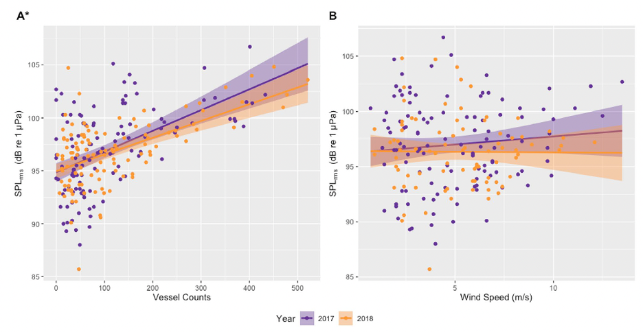
In addition to the data used in my previous three chapters collected from gray whales foraging off the Oregon coast, we also collected ambient noise levels using hydrophones, vessel count data from the Oregon Department of Fish and Wildlife (ODFW), and wind data from NOAA National Data Buoy Center (NDBC). Our first finding was a positive correlation between vessel counts and underwater noise levels (Fig. 1A), likely indicating that vessel traffic is the dominant source of noise in the area. To confirm this, we also compared underwater noise levels with wind speed (Fig. 1B), but no correlations were found.

**Figure 1:** Linear correlations between noise levels (daily median root mean square [rms] sound pressure level [SPL] in dB [re 1 μPa]; 50–1000 Hz) recorded on a hydrophone deployed outside the Newport harbor entrance during June to October of 2017 and 2018 and **(A)** vessel counts in Newport and Depoe Bay, Oregon, USA, and **(B)** daily median wind speed (m/s) from an anemometer station located on South Beach, Newport, Oregon, USA (station NWPO3). Asterisk indicates significant correlations between SPL and vessel counts in both years.

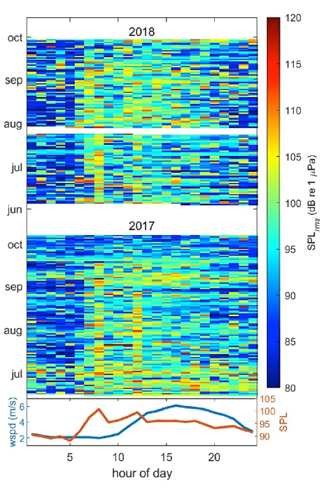
We also investigated noise levels by the hour of the day (Fig. 2), and we found that noise levels peaked between 6 and 8 am most days, coinciding with the peak of vessels leaving the harbor to get to fishing grounds. Another smaller peak is seen at 12 pm, which may represent “half-day fishing charter” vessels returning to the harbor. In contrast, wind speeds (in the lower graph) peaked between 3 and 4 pm, thus confirming the absence of correlation between noise and wind and providing more evidence that noise levels are dominated by the vessel activity in the area.

**Figure 2:** Median noise levels (root mean square sound pressure levels—SPLrms) for each hour of each day recorded on a hydrophone (50–10,000 Hz) deployed outside the Newport harbor entrance during June to October of 2017 (middle plot) and 2018 (upper plot), and hourly median noise level (SPL) against hourly median wind speed (lower plot) from an anemometer station located on South Beach, Newport, Oregon, USA (station NWPO3) over the same time period.

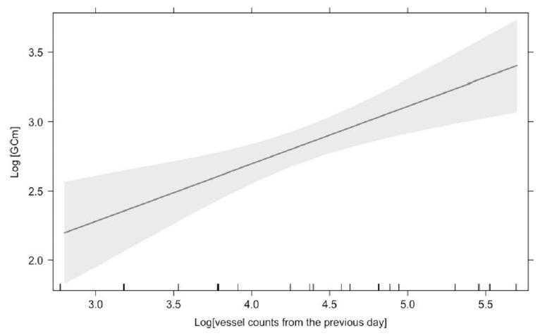
Finally, we assessed the effects of vessel counts, month, year, sex, whale body condition, and other hormone metabolites on glucocorticoid metabolite (GCm; “stress”) concentrations. Since we are working with fecal samples, we needed to consider the whale gut transit time and go back in time to link time of exposure (vessel counts) to response (glucocorticoid concentrations). However, due to uncertainty regarding gut transit time in baleen whales, we compared different time lags between vessel counts and fecal collection. The gut transit time in large mammals is ~12 hours to 4 days^3,19,20, so we investigated the influence of vessel counts on whale “stress hormone levels” from the previous 1 to 7 days. The model with the most influential temporal scale included vessel counts from previous day, which showed a significant positive relationship with GCm (the “stress hormone level”) (Fig. 3).

**Figure 3:** The effect of vessel counts in Newport and Depoe Bay (Oregon, USA) on the day before fecal sample collection on gray whale fecal glucocorticoid metabolite (GCm) concentrations.

Thus, the “take home messages” of our study are:

The soundscape in our study area is dominated by vessel noise.
Vessel counts are strongly correlated with ambient noise levels in our study area.
Gray whale glucocorticoid levels are positively correlated with vessel counts from previous day meaning that gray whale gut transit time may occur within ~ 24 hours of the disturbance event.

These four chapters were all very important studies not only to advance the knowledge of gray whale and overall baleen whale physiology (as this group is one of the most poorly understood of all mammals given the difficulties in sample collection²¹), but also to investigate potential sources for the unusual mortality event that is currently happening (2019-present) to the Eastern North Pacific population of gray whales. Such studies can be used to guide future research and to inform population management and conservation efforts regarding minimizing the impact of anthropogenic stressors on whales.

I am very glad to be part of this project, to see such great fruits from our gray whale research, and to know that this project is still at full steam. The GEMM Lab continues to collect and analyze data for determining gray whale body condition and physiological responses in association with ambient noise (Granite, Amber and Diamond projects). The gray whales thank you for this!

Cited Literature

1. McDonald, M. A., Hildebrand, J. A. & Wiggins, S. M. Increases in deep ocean ambient noise in the Northeast Pacific west of San Nicolas Island, California. J. Acoust. Soc. Am. 120, 711–718 (2006).

2. Kaplan, M. B. & Solomon, S. A coming boom in commercial shipping? The potential for rapid growth of noise from commercial ships by 2030. Mar. Policy 73, 119–121 (2016).

3. McCarthy, E. International regulation of underwater sound: establishing rules and standards to address ocean noise pollution (Kluwer Academic Publishers, 2004).

4. Weilgart, L. S. The impacts of anthropogenic ocean noise on cetaceans and implications for management. Can. J. Zool. 85, 1091–1116 (2007).

5. Bas, A. A. et al. Marine vessels alter the behaviour of bottlenose dolphins Tursiops truncatus in the Istanbul Strait, Turkey. Endanger. Species Res. 34, 1–14 (2017).

6. Erbe, C., Reichmuth, C., Cunningham, K., Lucke, K. & Dooling, R. Communication masking in marine mammals: a review and research strategy. Mar. Pollut. Bull. 103, 15–38 (2016).

7. Erbe, C. et al. The effects of ship noise on marine mammals: a review. Front. Mar. Sci. 6 (2019).

8. Sullivan, F. A. & Torres, L. G. Assessment of vessel disturbance to gray whales to inform sustainable ecotourism. J. Wildl. Manag. 82, 896–905 (2018).

9. Pirotta, E., Merchant, N. D., Thompson, P. M., Barton, T. R. & Lusseau, D. Quantifying the effect of boat disturbance on bottlenose dolphin foraging activity. Biol. Conserv. 181, 82–89 (2015).

10. Dans, S. L., Degrati, M., Pedraza, S. N. & Crespo, E. A. Effects of tour boats on dolphin activity examined with sensitivity analysis of Markov chains. Conserv. Biol. 26, 708–716 (2012).

11. Christiansen, F., Rasmussen, M. & Lusseau, D. Whale watching disrupts feeding activities of minke whales on a feeding ground. Mar. Ecol. Prog. Ser. 478, 239–251 (2013).

12. Bejder, L., Samuels, A., Whitehead, H. & Gales, N. Interpreting short-term behavioural responses to disturbance within a longitudinal perspective. Anim. Behav. 72, 1149–1158 (2006).

13. Nowacek, S. M., Wells, R. S. & Solow, A. R. Short-term effects of boat traffic on Bottlenose dolphins, Tursiops truncatus, in Sarasota Bay, Florida. Mar. Mammal. Sci. 17, 673–688 (2001).

14. Bejder, L., Dawson, S. M. & Harraway, J. A. Responses by Hector’s dolphins to boats and swimmers in Porpoise Bay, New Zealand. Mar. Mammal Sci. 15, 738–750 (1999).

15. Lusseau, D. Male and female bottlenose dolphins Tursiops spp. have different strategies to avoid interactions with tour boats in Doubtful Sound. New Zealand. Mar. Ecol. Prog. Ser. 257, 267–274 (2003).

16. Sprogis, K. R., Videsen, S. & Madsen, P. T. Vessel noise levels drive behavioural responses of humpback whales with implications for whale-watching. Elife 9, e56760 (2020).

17. Ayres, K. L. et al. Distinguishing the impacts of inadequate prey and vessel traffic on an endangered killer whale (Orcinus orca) population. PLoS ONE 7, e36842 (2012).

18. Rolland, R. M. et al. Evidence that ship noise increases stress in right whales. Proc. R. Soc. B Biol. Sci. 279, 2363–2368 (2012).

19. Wasser, S. K. et al. A generalized fecal glucocorticoid assay for use in a diverse array of nondomestic mammalian and avian species. Gen. Comp. Endocrinol. 120, 260–275 (2000).

20. Hunt, K. E., Trites, A. W. & Wasser, S. K. Validation of a fecal glucocorticoid assay for Steller sea lions (Eumetopias jubatus). Physiol. Behav. 80, 595–601 (2004).

21. Hunt, K. E. et al. Overcoming the challenges of studying conservation physiology in large whales: a review of available methods. Conserv. Physiol. 1, cot006–cot006 (2013).

Data Wrangling to Assess Data Availability: A Data Detective at Work

By Alexa Kownacki, Ph.D. Student, OSU Department of Fisheries and Wildlife, Geospatial Ecology of Marine Megafauna Lab

Data wrangling, in my own loose definition, is the necessary combination of both data selection and data collection. Wrangling your data requires accessing then assessing your data. Data collection is just what it sounds like: gathering all data points necessary for your project. Data selection is the process of cleaning and trimming data for final analyses; it is a whole new bag of worms that requires decision-making and critical thinking. During this process of data wrangling, I discovered there are two major avenues to obtain data: 1) you collect it, which frequently requires an exorbitant amount of time in the field, in the lab, and/or behind a computer, or 2) other people have already collected it, and through collaboration you put it to a good use (often a different use then its initial intent). The latter approach may result in the collection of so much data that you must decide which data should be included to answer your hypotheses. This process of data wrangling is the hurdle I am facing at this moment. I feel like I am a data detective.

Data wrangling illustrated by members of the R-programming community. (Image source: R-bloggers.com)

My project focuses on assessing the health conditions of the two ecotypes of bottlenose dolphins between the waters off of Ensenada, Baja California, Mexico to San Francisco, California, USA between 1981-2015. During the government shutdown, much of my data was inaccessible, seeing as it was in possession of my collaborators at federal agencies. However, now that the shutdown is over, my data is flowing in, and my questions are piling up. I can now begin to look at where these animals have been sighted over the past decades, which ecotypes have higher contaminant levels in their blubber, which animals have higher stress levels and if these are related to geospatial location, where animals are more susceptible to human disturbance, if sex plays a role in stress or contaminant load levels, which environmental variables influence stress levels and contaminant levels, and more!

Alexa, alongside collaborators, photographing transiting bottlenose dolphins along the coastline near Santa Barbara, CA in 2015 as part of the data collection process. (Image source: Nick Kellar).

Over the last two weeks, I was emailed three separate Excel spreadsheets representing three datasets, that contain partially overlapping data. If Microsoft Access is foreign to you, I would compare this dilemma to a very confusing exam question of “matching the word with the definition”, except with the words being in different languages from the definitions. If you have used Microsoft Access databases, you probably know the system of querying and matching data in different databases. Well, imagine trying to do this with Excel spreadsheets because the databases are not linked. Now you can see why I need to take a data management course and start using platforms other than Excel to manage my data.

A visual interpretation of trying to combine datasets being like matching the English definition to the Spanish translation. (Image source: Enchanted Learning)

In the first dataset, there are 6,136 sightings of Common bottlenose dolphins (Tursiops truncatus) documented in my study area. Some years have no sightings, some years have fewer than 100 sightings, and other years have over 500 sightings. In another dataset, there are 398 bottlenose dolphin biopsy samples collected between the years of 1992-2016 in a genetics database that can provide the sex of the animal. The final dataset contains records of 774 bottlenose dolphin biopsy samples collected between 1993-2018 that could be tested for hormone and/or contaminant levels. Some of these samples have identification numbers that can be matched to the other dataset. Within these cross-reference matches there are conflicting data in terms of amount of tissue remaining for analyses. Sorting these conflicts out will involve more digging from my end and additional communication with collaborators: data wrangling at its best. Circling back to what I mentioned in the beginning of this post, this data was collected by other people over decades and the collection methods were not standardized for my project. I benefit from years of data collection by other scientists and I am grateful for all of their hard work. However, now my hard work begins.

The cutest part of data wrangling: finding adorable images of bottlenose dolphins, photographed during a coastal survey. (Image source: Alexa Kownacki).

There is also a large amount of data that I downloaded from federally-maintained websites. For example, dolphin sighting data from research cruises are available for public access from the OBIS (Ocean Biogeographic Information System) Sea Map website. It boasts 5,927,551 records from 1,096 data sets containing information on 711 species with the help of 410 collaborators. This website is incredible as it allows you to search through different data criteria and then download the data in a variety of formats and contains an interactive map of the data. You can explore this at your leisure, but I want to point out the sheer amount of data. In my case, the OBIS Sea Map website is only one major platform that contains many sources of data that has already been collected, not specifically for me or my project, but will be utilized. As a follow-up to using data collected by other scientists, it is critical to give credit where credit is due. One of the benefits of using this website, is there is information about how to properly credit the collaborators when downloading data. See below for an example:

Example citation for a dataset (Dataset ID: 1201):

Lockhart, G.G., DiGiovanni Jr., R.A., DePerte, A.M. 2014. Virginia and Maryland Sea Turtle Research and Conservation Initiative Aerial Survey Sightings, May 2011 through July 2013. Downloaded from OBIS-SEAMAP (http://seamap.env.duke.edu/dataset/1201) on xxxx-xx-xx.

Citation for OBIS-SEAMAP:

Halpin, P.N., A.J. Read, E. Fujioka, B.D. Best, B. Donnelly, L.J. Hazen, C. Kot, K. Urian, E. LaBrecque, A. Dimatteo, J. Cleary, C. Good, L.B. Crowder, and K.D. Hyrenbach. 2009. OBIS-SEAMAP: The world data center for marine mammal, sea bird, and sea turtle distributions. Oceanography 22(2):104-115

Another federally-maintained data source that boasts more data than I can quantify is the well-known ERDDAP website. After a few Google searches, I finally discovered that the acronym stands for Environmental Research Division’s Data Access Program. Essentially, this the holy grail of environmental data for marine scientists. I have downloaded so much data from this website that Excel cannot open the csv files. Here is yet another reason why young scientists, like myself, need to transition out of using Excel and into data management systems that are developed to handle large-scale datasets. Everything from daily sea surface temperatures collected on every, one-degree of latitude and longitude line from 1981-2015 over my entire study site to Ekman transport levels taken every six hours on every longitudinal degree line over my study area. I will add some environmental variables in species distribution models to see which account for the largest amount of variability in my data. The next step in data selection begins with statistics. It is important to find if there are highly correlated environmental factors prior to modeling data. Learn more about fitting cetacean data to models here.

The ERDAPP website combined all of the average Sea Surface Temperatures collected daily from 1981-2018 over my study site into a graphical display of monthly composites. (Image Source: ERDDAP)

As you can imagine, this amount of data from many sources and collaborators is equal parts daunting and exhilarating. Before I even begin the process of determining the spatial and temporal spread of dolphin sightings data, I have to identify which data points have sex identified from either hormone levels or genetics, which data points have contaminants levels already quantified, which samples still have tissue available for additional testing, and so on. Once I have cleaned up the datasets, I will import the data into the R programming package. Then I can visualize my data in plots, charts, and graphs; this will help me identify outliers and potential challenges with my data, and, hopefully, start to see answers to my focal questions. Only then, can I dive into the deep and exciting waters of species distribution modeling and more advanced statistical analyses. This is data wrangling and I am the data detective.

What people may think a ‘data detective’ looks like, when, in reality, it is a person sitting at a computer. (Image source: Elder Research)

Like the well-known phrase, “With great power comes great responsibility”, I believe that with great data, comes great responsibility, because data is power. It is up to me as the scientist to decide which data is most powerful at answering my questions.

Share this:

Share this: