Barcelona-bound! The GEMM Lab heads to the World Marine Mammal Conference

By Dawn Barlow, PhD student, OSU Department of Fisheries and Wildlife, Geospatial Ecology of Marine Megafauna Lab

Every two years, an international community of scientists, managers, policy-makers, educators, and students gather to share the most current research and most pressing conservation issues facing marine mammals. This year, the World Marine Mammal Conference will take place in Barcelona, Spain from December 7-12, and the whole GEMM Lab will make their way across the Atlantic to present their latest work. The meeting is an international gathering of scientists ranging from longtime researchers who have shaped the field throughout the course of their careers to students who are just beginning to carve out a niche of their own. This year’s conference has 2,500 registered attendees from 95 different countries, 1,960 abstract submissions, and 700 accepted oral and speed talks and 1,200 posters. Needless to say, it is an incredible platform for learning, networking, and putting our work in the context of research taking place around the globe.

This will be my third time at this conference. I attended in San Francisco in 2015 as a wide-eyed undergraduate and met with Leigh, who I hoped would soon become my graduate advisor. I also presented my Masters research at the conference in Halifax in 2017. This time around, I will be presenting findings from the first two chapters of my PhD. Looking ahead to the Barcelona 2019 meeting and having some sense of what to expect, I feel butterflies rising in my stomach—a perfect mixture of the nerves that come with putting your hard work out in the world, eagerness to learn and absorb new information, and excitement to reconnect with friends and colleagues from around the world. In short, I can’t wait!

For those of you reading this blog that are unable to attend, I’d like to share an overview of what the GEMM Lab will be presenting at the conference. If you will be in Barcelona, we warmly invite you to the following posters, speed talks, and oral presentations! In order of appearance:

Lisa Hildebrand, MS Student

What do Oregon gray whales like to eat? Do individual whales have individual foraging habits? To learn more visit Lisa Hildebrand’s poster “Investigating potential gray whale individual foraging specializations within the Pacific Coast Feeding Group”. (Poster presentation, Session: Foraging Ecology – Group A, Time: Monday, 1:30-3:00pm)

Todd Chandler, Faculty Research Assistant

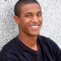
Did you know it is possible to measure the mechanics of how a blue whale feeds using a drone? The GEMM Lab’s all-star drone pilot Todd Chandler will present a poster titled “More than snacks: An analysis of drone observed blue whale surface lunge feeding linked with prey data”. (Poster presentation, Session: Foraging Ecology – Group A, Time: Monday, 1:30-3:00pm)

Clara Bird, MS Student

The GEMM Lab’s newest student Clara Bird will present a poster on work she conducted with the Marine Robotics and Remote Sensing lab at Duke University using new technologies and approaches to investigate scarring patterns on humpbacks. Her poster is titled “A comparison of percent dorsal scar cover between populations of humpback whales (Megaptera novaeangliae) off California and the Western Antarctic Peninsula”. (Poster presentation, Session: New Technology  – Group B, Time: Tuesday, 8:30-9:45am)

Dr. Leigh Torres, Principal Investigator

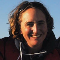
GEMM Lab PI Leigh Torres will synthesize some exciting new analyses from the GEMM Lab’s gray whale physiology and ecology research off the Oregon Coast. Is it stressful to feed in a noisy coastal environment? Leigh will discuss the latest findings in her talk, “Sounds of stress: Evaluating the relationships between variable soundscapes and gray whale stress hormones”. (Oral presentation, Session: Physiology, Time: Tuesday, 11:30-11:45am)

Leila Lemos, PhD Student

Carrying on with exciting new findings about Oregon gray whales, Leila Lemos will present a speed talk titled “Stressed and slim or relaxed and chubby? A simultaneous assessment of gray whale body condition and hormone variability”, in which she will summarize three years of analysis of how gray whale health can be quantified, and how physiology is influenced by ocean conditions. (Speed talk, Session: Physiology, Time: Tuesday, 11:55am-12:m)

Dawn Barlow, PhD Student

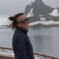
Can we predict where blue whales will be using our understanding of their environment and prey? Can this knowledge be used for effective conservation? I (Dawn Barlow) will give a presentation titled “Cloudy with a chance of whales: Forecasting blue whale occurrence based on tiered, bottom-up models to mitigate industrial impacts”, which will share our latest findings on how functional ecological relationships can be modeled in changing ocean conditions. (Oral presentation, Session: Habitat and Distribution I, Time: Wednesday, 10:15-10:30am)

Dr. Solene Derville, Post-Doctoral Scholar

The GEMM Lab’s most recent graduate Solene Derville will present work she has conducted in New Caledonia regarding humpback whale diving and movement patterns around breeding grounds. Her speed talk is titled “Whales of the deep: Horizontal and vertical movements shed light on humpback whale use of critical pelagic habitats in the western South Pacific” (Speed talk, Session: Behavioral Ecology II, Time: Wednesday, 11:35-11:40am)

Dominique Kone, MS Student

Can sea otters make a comeback in Oregon after a long absence? Dom Kone takes a comprehensive look at how Oregon coast habitat could support a reintroduced sea otter population in his speed talk, “An evaluation of the ecological needs and effects of a potential sea otter reintroduction to Oregon, USA”. (Speed talk, Session: Conservation II, Time: Wednesday, 2:45-2:50pm)

Alexa Kownacki, PhD Student

Alexa Kownacki will share her latest findings on dolphin distribution relative to static and dynamic oceanographic variables in her speed talk titled “The biogeography of common bottlenose dolphins (T. truncatus) of the southwestern USA and Mexico”. (Speed talk, Session: Habitat and Distribution II, Time: Wednesday, 3:35-3:40pm)

Other members of the Marine Mammal Mnstitute who will present their work include: Scott Baker, Debbie Steel, Angie Sremba, Karen Lohman, Daniel Palacios, Bruce Mate, Ladd Irvine, and Robert Pitman. For anyone planning to attend, we look forward to seeing you there! For those who wish to stay tuned from home, keep your eye on the GEMM Lab twitter page for our updates during the conference and follow the conference hashtag #WMMC19, and look forward to future blog posts recapping the experience.

Detecting blue whales from acoustic data

By Dawn Barlow, PhD student, OSU Department of Fisheries and Wildlife, Geospatial Ecology of Marine Megafauna Lab

In January of 2016, five underwater recording units were dropped to the seafloor in New Zealand to listen for blue whales (Fig. 1). These hydrophones sat listening for two years, brought to the surface only briefly every six months to swap out batteries and offload the data. Through all seasons and conditions when scientists couldn’t be on the water, they recorded the soundscape, generating a wealth of acoustic data with the potential to greatly expand our knowledge of blue whale ecology

Figure 1. Locations of the five Marine Autonomous Recording Units (MARUs) in the South Taranaki Bight region of New Zealand.

We have established that blue whales are present in New Zealand waters year-round 1. However, many questions remain regarding their distribution across daily, seasonal, and yearly scales. Our two-year acoustic dataset from five hydrophones throughout the STB region is a goldmine of information on blue whale occurrence patterns and the soundscape they inhabit. Having year-round occurrence data will allow us to examine what environmental and anthropogenic factors may influence blue whale distribution patterns. The hydrophones were listening for whales around the clock, every day, while we were on the other side of the world awaiting the recovery of the data to answer our questions.

Before any questions of seasonal distribution or anthropogenic impacts and noise can be addressed, however, we need to know something far more basic: when and where did we record blue whale vocalizations? This may seem like a simple, stepping-stone question, but it is actually quite involved, and the reason I spent the last month working with a team of acousticians at Cornell University’s Center for Conservation Bioacoustics. The expert research group here at Cornell, led by Dr. Holger Klinck, have been instrumental in our New Zealand blue whale research, including developing and building the recording units, hydrophone deployment and recovery, data processing, analysis, and advice. I am thrilled to work with all of them, and had an incredibly productive month of learning about acoustics from the best.

Blue whales produce multiple vocalizations that we are interested in documenting. The New Zealand song (Fig. 2A) is highly stereotyped and unique to the Southwest Pacific Ocean 2,3. Low-frequency downsweeps, or “D calls” (Fig. 2B), are far more variable and produced by blue whale populations around the world 4. Furthermore, Antarctic blue whales produce a highly-stereotyped “Z call” (Fig. 2C) and are known to be present in New Zealand waters occasionally 5.

Figure 2. Spectrograms of (A) the New Zealand blue whale song, (B), D calls, and (C) Antarctic Z calls.

One way to determine when blue whales were vocalizing is for an analyst to manually review the entirety of the two years of sound recordings for each of the five hydrophones by hand to scan for and select individual vocalizations. An alternative approach is to develop a detector algorithm to locate calls in the data based on their stereotypical characteristics. Over the past month I built, tested, and ran detectors for each blue whale call type using what is called a data template detector. This technique uses example signals from the data that the analyst selects as templates. The templates should be clear signals, and representative of the variation in calls contained in the dataset. Then, by comparing pixel characteristics between the template spectrograms and the spectrogram of the recording of interest using certain matching criteria (e.g. threshold for spectrogram correlation, detection frequency range), the algorithm searches for other signals like the templates in the full dataset. For example, in Fig. 3 you can see units of blue whale song I selected as templates for my detector.

Figure 3. Spectrogram of selected sound clips of New Zealand blue whale song, with units used as templates for a detector shown inside the teal boxes.

Testing the performance of a detector algorithm is critical. Therefore, a dataset is needed where calls were identified by an analyst and then used as the “ground truth”, to which the detector results are compared. For my ground truth dataset, I took a subset of 52 days and hand-browsed the spectrograms to identify and log New Zealand blue whale song, D calls, and Antarctic Z calls. In evaluating detector performance, there are three important metrics that need to be weighed: precision (the proportion of detections that are true), recall (the proportion of true calls identified by the detector), and false alarm rate (the number of false positive detections per hour). Ideally, the detector should be optimized to maximize precision and recall and minimize the false positives.

The STB region is highly industrial, and our two-year acoustic dataset contains periods of pervasive seismic airgun noise from oil and gas exploration. Ideally, a detector would be able to identify blue whale vocalizations even in the presence of airgun operations that dominate the soundscape for months. For blue whale song, the detector did quite well! With a precision of 0.91 and recall of 0.93, the detector could pick out song units over airgun noise (Fig. 4). A false alarm rate of 8 false positives per hour is a sacrifice worth making to identify song during seismic operations (and the false positives will be removed in a subsequent step). For D calls, seismic survey activity presented a different challenge. While the detector did well at identifying D calls during airgun operation, the first several detector attempts also logged every single airgun blast as a blue whale vocalization—clearly problematic. Through an iterative process of selecting template signals, and adjusting the number of templates used and the correlation threshold, I was able to come up with a detector which selected D calls and missed most airgun blasts. This success felt like a victory.

Figure 4. An example of spectrograms of simultaneous recordings from the five hydrophones illustrating seismic airgun noise (strong broadband signals that appear as repetitive black, vertical lines) overlapping New Zealand blue whale song. The red boxes are detection events selected by the detector, demonstrating its ability to capture song even during airgun operation.

After this detector development and validation process, I ran each detector on the full two-year acoustic dataset for all five recording units. This step was a good exercise in patience as I eagerly awaited the outputs for the many hours they took to run. The next step in the process will be for me to go through and validate each detector event to eliminate any false positives. However, running the detectors on the full dataset has allowed for exciting preliminary examinations of seasonal blue whale acoustic patterns, which need to be refined and expanded upon as the analysis continues. For example, sometimes the New Zealand song dominates the recordings on all hydrophones (Fig. 5), whereas other times of year song is less common. Similarly, there appear to be seasonal patterns in D calls and Antarctic Z calls, with peaks and dips in detections during different times of year.

Figure 5. An example spectrogram of simultaneous recordings from all five hydrophones during a time when New Zealand blue whale song dominated the recordings, with numerous, overlapping calls.

As with many things, the more questions you ask, the more questions you come up with. From preliminary explorations of the acoustic data my head is buzzing with ideas for further analysis and with new questions I hadn’t thought to ask of the data before. My curiosity has been fueled by scrolling through spectrograms, looking, and listening, and I am as excited as ever to continue researching blue whale ecology. I would like to thank the team at the Center for Conservation Bioacoustics for their support and guidance over the past month, and I look forward to digging deeper into the stories being told in the acoustic data!

Figure 6. A pair of blue whales observed in February 2017 in the South Taranaki Bight. Photo: L. Torres.

References

1.          Barlow, D. R. et al. Documentation of a New Zealand blue whale population based on multiple lines of evidence. Endanger. Species Res. 36, 27–40 (2018).

2.          McDonald, M. A., Mesnick, S. L. & Hildebrand, J. A. Biogeographic characterisation of blue whale song worldwide: using song to identify populations. J. Cetacean Res. Manag. 8, 55–65 (2006).

3.          Balcazar, N. E. et al. Calls reveal population structure of blue whales across the Southeast Indian Ocean and the Southwest Pacific Ocean. J. Mammal. 96, 1184–1193 (2015).

4.          Oleson, E. M. et al. Behavioral context of call production by eastern North Pacific blue whales. Mar. Ecol. Prog. Ser. 330, 269–284 (2007).

5.          McDonald, M. A. An acoustic survey of baleen whales off Great Barrier Island, New Zealand. New Zeal. J. Mar. Freshw. Res. 40, 519–529 (2006).


Eyes from Space: Using Remote Sensing as a Tool to Study the Ecology of Blue Whales

By Christina Garvey, University of Maryland, GEMM Lab REU Intern

It is July 8th and it is my 4th week here in Hatfield as an REU intern for Dr. Leigh Torres. My name is Christina Garvey and this summer I am studying the spatial ecology of blue whales in the South Taranaki Bight, New Zealand. Coming from the east coast, Oregon has given me an experience of a lifetime – the rugged shorelines continue to take my breath away and watching sea lions in Yaquina Bay never gets old. However, working on my first research project has by far been the greatest opportunity and I have learned so much in so little time. When Dr. Torres asked me to contribute to this blog I was unsure of how I would write about my work thus far but I am excited to have the opportunity to share the knowledge I have gained with whoever reads this blog post.

The research project that I will be conducting this summer will use remotely sensed environmental data (information collected from satellites) to predict blue whale distribution in the South Taranaki Bight (STB), New Zealand. Those that have read previous blogs about this research may remember that the STB study area is created by a large indentation or “bight” on the southern end of the Northern Island. Based on multiple lines of evidence, Dr. Leigh Torres hypothesized the presence of an unrecognized blue whale foraging ground in the STB (Torres 2013). Dr. Torres and her team have since proved that blue whales frequent this region year-round; however, the STB is also very industrial making this space-use overlap a conservation concern (Barlow et al. 2018). The increasing presence of marine industrial activity in the STB is expected to put more pressure on blue whales in this region, whom are already vulnerable from the effects of past commercial whaling (Barlow et al. 2018) If you want to read more about blue whales in the STB check out previous blog posts that talk all about it!

Figure 1. A blue whale surfaces in front of a floating production storage and offloading vessel servicing the oil rigs in the South Taranaki Bight. Photo by D. Barlow.

Figure 2. South Taranaki Bight, New Zealand, our study site outlined by the red box. Kahurangi Point (black star) is the site of wind-driven upwelling system.

The possibility of the STB as an important foraging ground for a resident population of blue whales poses management concerns as New Zealand will have to balance industrial growth with the protection and conservation of a critically endangered species. As a result of strong public support, there are political plans to implement a marine protected area (MPA) in the STB for the blue whales. The purpose of our research is to provide scientific knowledge and recommendations that will assist the New Zealand government in the creation of an effective MPA.

In order to create an MPA that would help conserve the blue whale population in the STB, we need to gather a deeper understanding of the relationship between blue whales and this marine environment. One way to gain knowledge of the oceanographic and ecological processes of the ocean is through remote sensing by satellites, which provides accessible and easy to use environmental data. In our study we propose remote sensing as a tool that can be used by managers for the design of MPAs (through spatial and temporal boundaries). Satellite imagery can provide information on sea surface temperature (SST), SST anomaly, as well as net primary productivity (NPP) – which are all measurements that can help describe oceanographic upwelling, a phenomena that is believed to be correlated to the presence of blue whales in the STB region.

Figure 3. The stars of the show: blue whales. A photograph captured from the small boat of one animal fluking up to dive down as another whale surfaces close by. (Photo credit: L. Torres)

Past studies in the STB showed evidence of a large upwelling event that occurs off the coast of Kahurangi Point (Fig. 2), on the northwest tip of the South Island (Shirtcliffe et al. 1990). In order to study the relationship of this upwelling to the distribution of blue whales, I plan to extract remotely sensed data (SST, SST anomaly, & NPP) off the coast of Kahurangi and compare it to data gathered from a centrally located site within the STB, which is close to oil rigs and so is of management interest. I will first study how decreases in sea surface temperature at the site of upwelling (Kahurangi) are related to changes in sea surface temperature at this central site in the STB, while accounting for any time differences between each occurrence. I expect that this relationship will be influenced by the wind patterns, and that there will be changes based on the season. I also predict that drops in temperature will be strongly related to increases in primary productivity, since upwelling brings nutrients important for photosynthesis up to the surface. These dips in SST are also expected to be correlated to blue whale occurrence within the bight, since blue whale prey (krill) eat the phytoplankton produced by the productivity.

Figure 4. A blue whale lunges on an aggregation of krill. UAS piloted by Todd Chandler.

To test the relationships I determine between remotely sensed data at different locations in the STB, I plan to use blue whale observations from marine mammal observers during a seismic survey conducted in 2013, as well as sightings recorded from the 2014, 2016, and 2017 field studies led by Dr. Leigh Torres. By studying the statistical relationships between all of these variables I hope to prove that remote sensing can be used as a tool to study and understand blue whale distribution.

I am very excited about this research, especially because the end goal of creating an MPA really gives me purpose. I feel very lucky to be part of a project that could make a positive impact on the world, if only in just a little corner of New Zealand. In the mean time I’ll be here in Hatfield doing the best I can to help make that happen.

References: 

Barlow DR, Torres LG, Hodge KB, Steel D, Baker CS, Chandler TE, Bott N, Constantine R, Double MC, Gill P, Glasgow D, Hamner RM, Lilley C, Ogle M, Olson PA, Peters C, Stockin KA, Tessaglia-hymes CT, Klinck H (2018) Documentation of a New Zealand blue whale population based on multiple lines of evidence. Endanger Species Res 36:27–40.

Shirtcliffe TGL, Moore MI, Cole AG, Viner AB, Baldwin R, Chapman B (1990) Dynamics of the Cape Farewell upwelling plume, New Zealand. New Zeal J Mar Freshw Res 24:555–568.

Torres LG (2013) Evidence for an unrecognised blue whale foraging ground in New Zealand. New Zeal J Mar Freshw Res 47:235–248.

Species distribution modeling: Part statistics, part philosophy, and there is no “right answer”

By Dawn Barlow, PhD student, OSU Department of Fisheries and Wildlife, Geospatial Ecology of Marine Megafauna Lab

Just like that, I have wrapped up year 1 of my PhD in Wildlife Science. For my PhD, I am investigating the ecology and distribution of blue whales in New Zealand across multiple spatial and temporal scales. In a region where blue whales overlap with industrial activity, there is considerable interest from managers to be able to reliably forecast when and where blue whales are most likely to be in the area. In a series of five chapters and utilizing multiple different data sources (dedicated boat surveys, oceanographic data, acoustic recordings, remotely sensed environmental data, opportunistic blue whale sightings information), I will attempt to describe, quantify, and predict where blue whales are found in relation to their environment. Each chapter will evaluate the distribution of blue whales relative to the environment at different scales in space (ranging from 4 km to 25 km resolution) and time (ranging from daily to seasonal resolution). One overarching method I am using throughout my PhD is species distribution modeling. Having just completed my research review with my doctoral committee last week, I’ll share this aspect of my research proposal that I’ve particularly enjoyed reading, writing, and thinking about.

A pair of blue whales surfacing in the South Taranaki Bight region of New Zealand. Drone piloted by Todd Chandler during the 2017 field season.

Species distribution models (SDMs), which are sometimes referred to as habitat models or ecological niche models, are mathematical algorithms that combine observations of a species with environmental conditions at their observed locations, to gain ecological insight and predict spatial distributions of the species (Elith and Leathwick, 2009; Redfern et al., 2006). Any model is just one description of what is occurring in the natural world. Just as there are many ways to describe something with words and many languages to do so, there are many options for modeling frameworks and approaches, with stark and nuanced differences. My labmate and friend Solene Derville has equated the number of choices one has for SDMs to the cracker section in an American grocery store. When navigating all of these choices and considerations, it is important to remember that no model will ever be completely correct—it is our best attempt at describing a complex natural system—and as an analyst we need to do the best that we can with the data available to address the ecological questions at hand. As it turns out, the dividing line between quantitative analysis and philosophy is thin at times. What may seem at first like a purely objective, statistical endeavor requires careful consideration and fundamental decision-making on the part of the analyst.

Ecosystems are multifaceted, complex, and hierarchical. They are comprised of multiple physical and biological components, which operate at multiple scales across space and time. As Dr. Simon Levin stated in at 1989 MacArthur Award lecture on the topic of scale in ecology:

“A good model does not attempt to reproduce every detail of the biological system; the system itself suffices for that purpose as the most detailed model of itself. Rather, the objective of a model should be to ask how much detail can be ignored without producing results that contradict specific sets of observations, on particular scales of interest” (Levin, 1992).

The question of scale is central to ecology. As many biology students learn in their first introductory classes, parsimony is “The principle that the most acceptable explanation of an occurrence, phenomenon, or event is the simplest, involving the fewest entities, assumptions, or changes” (Oxford Dictionary). In other words, the best explanation is the simplest one. One challenge in ecological modeling, including SDMs, is to select spatial and temporal scales as coarse as possible for the most parsimonious—the most straightforward—model, while still being fine enough to capture relevant patterns. Another critical consideration is the scale of the question you are interested in answering. The scale of the analysis must match the scale at which you want to make inferences about the ecology of a species.

Similarly, the issue of complexity is central to distribution modeling. Overly simple models may not be able to adequately describe the relationship between species occurrence and the environment. In contrast, highly complex models may have very high explanatory power, but risk ascribing an ecological pattern to noise in the data (Merow et al., 2014), in other words, finding patterns that aren’t real. Furthermore, highly complex models tend to have poorer predictive capacity than simpler models (Merow et al., 2014). There is a trade-off between descriptive and predictive power in SDMs (Derville et al., 2018). Therefore, a key component in the SDM process is establishing the end goal of the model with respect to the region of interest, scale, explanatory power, predictive capacity, and in many cases management need.

Finally, any model is ultimately limited by the data available and the scale at which it was collected (Elith and Leathwick, 2009; Guillera-Arroita et al., 2015; Redfern et al., 2006). Prior knowledge of what environmental features are important to the species of interest is often limited at the time of the data collection effort, and data collection is constrained by when it is logistically feasible to sample. For example, we collect detailed oceanographic data during the summer months when it is practical to get out on the water, satellite imagery of sea surface temperature might be unavailable during times of cloud cover, and people are more likely to report blue whale sightings in areas where there is more human activity. Therefore, useful SDMs that address both ecological and management needs typically balance the scale of analysis and model complexity with the limitations of the data.

Managers and politicians within the New Zealand government are interested in a tool to predict when and where blue whales are most likely to be, based on sound ecological analysis. This is one of the end-goals of my PhD, but in the meantime, I am grappling with the appropriate scales of analysis, and attempting to balance questions of model complexity, explanatory power, and predictive capacity. There is no single, correct answer, and so my process is in part quantitative analysis, part philosophy, and all with the goal of increased ecological understanding and conservation of a species.

A blue whale breaks the surface. As I grapple with questions of model complexity and scale of analysis, I sometimes need a reminder that behind each data point is a blue whale, and what a privilege it is to study them. Photo by Leigh Torres.

References:

Derville, S., Torres, L. G., Iovan, C., and Garrigue, C. (2018). Finding the right fit: Comparative cetacean distribution models using multiple data sources and statistical approaches. Divers. Distrib. 24, 1657–1673. doi:10.1111/ddi.12782.

Elith, J., and Leathwick, J. R. (2009). Species Distribution Models: Ecological Explanation and Prediction Across Space and Time. Annu. Rev. Ecol. Evol. Syst. 40, 677–697. doi:10.1146/annurev.ecolsys.110308.120159.

Guillera-Arroita, G., Lahoz-Monfort, J. J., Elith, J., Gordon, A., Kujala, H., Lentini, P. E., et al. (2015). Is my species distribution model fit for purpose? Matching data and models to applications. Glob. Ecol. Biogeogr. 24, 276–292. doi:10.1111/geb.12268.

Levin, S. A. (1992). The problem of pattern and scale. Ecology 73, 1943–1967.

Merow, C., Smith, M. J., Edwards, T. C., Guisan, A., Mcmahon, S. M., Normand, S., et al. (2014). What do we gain from simplicity versus complexity in species distribution models? Ecography (Cop.). 37, 1267–1281. doi:10.1111/ecog.00845.

Redfern, J. V., Ferguson, M. C., Becker, E. A., Hyrenbach, K. D., Good, C., Barlow, J., et al. (2006). Techniques for cetacean-habitat modeling. Mar. Ecol. Prog. Ser. 310, 271–295. doi:10.3354/meps310271.

The “demon whale-biter”, and why I am learning about an elusive little shark

By Dawn Barlow, PhD student, OSU Department of Fisheries and Wildlife, Geospatial Ecology of Marine Megafauna Lab

There is an ancient Samoan legend that upon entry into a certain bay in Samoa, tuna would sacrifice pieces of their flesh to the community chief1. This was the explanation given for fish with circular shaped wounds where a plug of flesh had been removed. Similar round wounds are also observed on swordfish2, sharks3, and marine mammals including whales4,5, dolphins6, porpoises7, and pinnipeds8,9. In 1971, Everet C. Jones posited that the probable cause of these crater wounds was a small shark only 42-56 cm in length, Isistius brasiliensis1. The species was nicknamed “demon whale-biter” by Stewart Springer, who subsequently popularized the common name for the species, cookie cutter shark.

Figure 1. A yellowfin tuna with a circular bite, characteristic of a cookie cutter shark (Isistius brasiliensis). Photo: John Soward.

I am currently preparing a manuscript on blue whale skin condition. While this is only tangentially related to my doctoral research, it is an exciting side project that has encouraged me to stretch my comfort zone as an ecologist. This analysis of skin condition is part of a broader health assessment of blue whales in New Zealand, where we will be linking skin lesion severity with stress and reproductive hormone levels as well as body condition. Before I continue, I owe a major shout-out to Acacia Pepper, a senior undergraduate student at Oregon State University who has been working with me for nearly the past year through the Fisheries and Wildlife mentorship program. Acacia’s rigor in researching methodologies led us to develop a comprehensive protocol that can be applied widely to any cetacean photo-identification catalog. This method allows us to quantify prevalence and severity of different marking types in a standardized manner. Her passion for marine mammal science and interest in the subject matter is enough to excite this ecologist into fascination with wound morphology and blister concavity. Next thing you know, we are preparing a paper for publication together with P.I. Dr. Leigh Torres on a comprehensive skin condition assessment of blue whales that includes multiple markings and lesion types, but for the purpose of this blog post, I will share just a “bite-sized” piece of the story.

Figure 2. Jaws of a cookie cutter shark. Photo: George Burgess.

Back to the demon whale-biter. What do we know about cookie cutter sharks? Not a whole lot, it turns out. They are elusive, and are thought to live in deep (>1,000 m), offshore waters. They are considered to be both an ectoparasite and an ambush predator. Their distribution is tropical and sub-tropical. Much of what we know and assume about their distribution comes from the bite wounds they leave on their prey2.

In New Zealand where we study a unique population of blue whales10, the southernmost record of cookie cutter sharks is ~ 39⁰S11. We found that in our dataset of 148 photo-identified blue whales, 96% were affected by cookie cutter shark bites. Furthermore, 38% were categorized as having “severe” cookie cutter bite wounds or scars. The latitude of our blue whale sightings ranges from 29-48⁰S and blue whales are highly mobile, so any of the whales in our dataset could theoretically swim in and out of the known range of cookie cutter sharks. In our skin condition assessment, we also categorized cookie cutter bite “freshness” and phase of healing as follows:

We wanted to know if the freshness of cookie cutter shark bites was related in to the latitude at which the whales were photographed. Of the whales photographed north of 39⁰S (n=46), 76% had phase 1 or 2 cookie cutter shark bites present. In contrast, 57.1% of whales photographed south of 39⁰S (n=133) had phase 1 or 2 cookie cutter shark bites. It therefore appears that in New Zealand, the freshness of cookie cutter shark bites on blue whales is related to the latitude at which the whales were sighted, with fresher bites being more common at more northerly latitudes.

Figure 3. A whale with fresh cookie cutter shark bites, photographed in the Bay of Islands, latitude 35.164⁰S. Photo courtesy of Dr. Catherine Peters.

Figure 4. A whale with mostly healed cookie cutter shark bites, photographed off of Kaikoura, latitude 42.464⁰S. Photo courtesy of Jody Weir.

In the midst of a PhD on distribution modeling and habitat use of blue whales, I find myself reading about Samoan legends of tuna with missing flesh and descriptions of strange circular lesions from whaling records, and writing a paper about blue whale skin condition. Exciting “side projects” like this one emerge from rich datasets and good collaboration.

References

  1. Jones, E. C. Isistius brasiliensis, a squaloid shark, the probable cause of crater wounds on fishes and cetaceans. Fish. Bull. 69, 791–798 (1971).
  2. Papastamatiou, Y. P., Wetherbee, B. M., O’Sullivan, J., Goodmanlowe, G. D. & Lowe, C. G. Foraging ecology of Cookiecutter Sharks (Isistius brasiliensis) on pelagic fishes in Hawaii, inferred from prey bite wounds. Environ. Biol. Fishes 88, 361–368 (2010).
  3. Hoyos-Padilla, M., Papastamatiou, Y. P., O’Sullivan, J. & Lowe, C. G. Observation of an Attack by a Cookiecutter Shark ( Isistius brasiliensis ) on a White Shark ( Carcharodon carcharias ) . Pacific Sci. 67, 129–134 (2013).
  4. Mackintosh, N. A. & Wheeler, J. F. G. Southern blue and fin whales. Discov. Reports 1, 257–540 (1929).
  5. Best, P. B. & Photopoulou, T. Identifying the ‘demon whale-biter’: Patterns of scarring on large whales attributed to a cookie-cutter shark Isistius sp. PLoS One 11, (2016).
  6. Heithaus, M. R. Predator-prey and competitive interactions between sharks (order Selachii) and dolphins (suborder Odontoceti): A review. J. Zool. 253, 53–68 (2001).
  7. Van Utrecht, W. L. Wounds And Scars In The Skin Of The Common Porpoise, Phocaena Phocaena (L.). Mammalia 23, 100–122 (1959).
  8. Gallo‐Reynoso, J. ‐P & Figueroa‐Carranza, A. ‐L. A COOKIECUTTER SHARK WOUND ON A GUADALUPE FUR SEAL MALE. Mar. Mammal Sci. 8, 428–430 (1992).
  9. Le Boeuf, B. J., McCosker, J. E. & Hewitt, J. Crater wounds on northern elephant seals: the cookiecutter shark strikes again. Fish. Bull. 85, 387–392 (1987).
  10. Barlow, D. R. et al. Documentation of a New Zealand blue whale population based on multiple lines of evidence. Endanger. Species Res. 36, 27–40 (2018).
  11. Dwyer, S. L. & Visser, I. N. Cookie cutter shark (Isistius sp.) bites on cetaceans, with particular reference to killer whales (Orca) (Orcinus orca). Aquat. Mamm. 37, 111–138 (2011).

More data, more questions, more projects: There’s always more to learn

By Dawn Barlow, PhD student, OSU Department of Fisheries and Wildlife, Geospatial Ecology of Marine Megafauna Lab 

As you may have read in previous blog posts, my research focuses on the ecology of blue whales in New Zealand. Through my MS research and years of work by a dedicated team, we were able to document and describe a population of around 700 blue whales that are unique to New Zealand, present year-round, and genetically distinct from all other known populations [1]. While this is a very exciting discovery, documenting this population has also unlocked a myriad of further questions about these whales. Can we predict when and where the whales are most likely to be? How does their distribution change seasonally? How often do they overlap with anthropogenic activity? My PhD research will aim to answer these questions through models of blue whale distribution patterns relative to their environment at multiple spatial and temporal scales.

Because time at sea for vessel-based surveys is cost-limited and difficult to come by, it is in any scientist’s best interest to collect as many concurrent streams of data as possible while in the field. When Dr. Leigh Torres designed our blue whale surveys that were conducted in 2014, 2016, and 2017, she really did a miraculous job of maximizing time on the water. With more data, more questions can be asked. These complimentary datasets have led to the pursuit of many “side projects”. I am lucky enough to work on these questions in parallel with what will form the bulk of my PhD, and collaborate with a number of people in the process. In this blog post, I’ll give you some short teasers of these “side projects”!

Surface lunge feeding as a foraging strategy for New Zealand blue whales

Most of what we know about blue whale foraging behavior comes from studies conducted off the coast of Southern California[2,3] using suction cup accelerometer tags. While these studies in the California Current ecosystem have led to insights and breakthroughs in our understanding of these elusive marine predators and their prey, they have also led us to adopt the paradigm that krill patches are denser at depth, and blue whales are most likely to target these deep prey patches when they feed. We have combined our prey data with blue whale behavioral data observed via a drone to investigate blue whale foraging in New Zealand, with a particular emphasis on surface feeding as a strategy. In our recent analyses, we are finding that in New Zealand, lunge feeding at the surface may be more than just “snacking”. Rather, it may be an energetically efficient strategy that blue whales have evolved in the region with unique implications for conservation.

Figure 1. A blue whale lunges on an aggregation of krill. UAS piloted by Todd Chandler.

Combining multiple data streams for a comprehensive health assessment

In the field, we collected photographs, blubber biopsy samples, fecal samples, and conducted unmanned aerial system (UAS, a.k.a. “drone”) flights over blue whales. The blubber and fecal samples can be analyzed for stress and reproductive hormone levels; UAS imagery allows us to quantify a whale’s body condition[4]; and photographs can be used to evaluate skin condition for abnormalities. By pulling together these multiple data streams, this project aims to establish a baseline understanding of the variability in stress and reproductive hormone levels, body condition, and skin condition for the population. Because our study period spans multiple years, we also have the ability to look at temporal patterns and individual changes over time. From our preliminary results, we have evidence for multiple pregnant females from elevated pregnancy and stress hormones, as well as apparent pregnancy from the body condition analysis. Additionally, a large proportion of the population appear to be affected by blistering and cookie cutter shark bites.

Figure 2. An example aerial drone image of a blue whale that will be used to asses body condition, i.e. how healthy or malnourished the whale is. (Drone piloted by Todd Chandler).

Figure 3. Images of blue whale skin condition, affected by A) blistering and B) cookie cutter shark bites.

Comparing body shape and morphology between species

The GEMM Lab uses UAS to quantitatively study behavior[5] and health of large whales. From various projects in different parts of the world we have now assimilated UAS data on blue, gray, and humpback whales. We will measure these images to investigate differences in body shape and morphology among these species. We plan to explore how form follows function across baleen whales, based on their different  life histories, foraging strategies, and ecological roles.

Figure 4 . Aerial images of A) a blue whale in New Zealand’s South Taranaki Bight, B) a gray whale off the coast of Oregon, and C) a humpback whale off the coast of Washington. Drone piloted by Todd Chandler (A and B) and Jason Miranda (C). 

So it goes—my dissertation will contain a series of chapters that build on one another to explore blue whale distribution patterns at increasing scales, as well as a growing number of appendices for these “side projects”. Explorations and collaborations like I’ve described here allow me to broaden my perspectives and diversify my analytical skills, as well as work with many excellent teams of scientists. The more data we collect, the more questions we are able to ask. The more questions we ask, the more we seem to uncover that is yet to be understood. So stay tuned for some exciting forthcoming results from all of these analyses, as well as plenty of new questions, waiting to be posed.

References

  1. Barlow DR et al. 2018 Documentation of a New Zealand blue whale population based on multiple lines of evidence. Endanger. Species Res. 36, 27–40. (doi:https://doi.org/10.3354/esr00891)
  2. Hazen EL, Friedlaender AS, Goldbogen JA. 2015 Blue whales (Balaenoptera musculus) optimize foraging efficiency by balancing oxygen use and energy gain as a function of prey density. Sci. Adv. 1, e1500469–e1500469. (doi:10.1126/sciadv.1500469)
  3. Goldbogen JA, Calambokidis J, Oleson E, Potvin J, Pyenson ND, Schorr G, Shadwick RE. 2011 Mechanics, hydrodynamics and energetics of blue whale lunge feeding: efficiency dependence on krill density. J. Exp. Biol. 214, 131–146. (doi:10.1242/jeb.048157)
  4. Burnett JD, Lemos L, Barlow DR, Wing MG, Chandler TE, Torres LG. 2018 Estimating morphometric attributes on baleen whales using small UAS photogrammetry: A case study with blue and gray whales. Mar. Mammal Sci. (doi:10.1111/mms.12527)
  5. Torres LG, Nieukirk SL, Lemos L, Chandler TE. 2018 Drone Up! Quantifying Whale Behavior From a New Perspective Improves Observational Capacity. Front. Mar. Sci. 5. (doi:10.3389/fmars.2018.00319)

More than just whales: The importance of studying an ecosystem


By Dawn Barlow, PhD student, OSU Department of Fisheries and Wildlife, Geospatial Ecology of Marine Megafauna Lab

I have the privilege of studying the largest animals on the planet: blue whales (Balaenoptera musculus). However, in order to understand the ecology, distribution, and habitat use patterns of these ocean giants, I have dedicated the past several months to studying something much smaller: krill (Nyctiphanes australis). New Zealand’s South Taranaki Bight region (“STB”, Figure 1) is an important foraging ground for a unique population of blue whales [1,2]. A wind-driven upwelling system off of Kahurangi Point (the “X” in Figure 1) generates productivity in the region [3], leading to an abundance of krill [4], the desired blue whale prey [5].

Our blue whale research team collected a multitude of datastreams in three different years, including hydroacoustic data to map krill distribution throughout our study region. The summers of 2014 and 2017 were characterized by what could be considered “typical” conditions: A plume of cold, upwelled water curving its way around Cape Farewell (marked with the star in Figure 1) and entering the South Taranaki Bight, spurring a cascade of productivity in the region. The 2016 season, however, was different. The surface water temperatures were hot, and the whales were not where we expected to find them.

Figure 2. Sea surface temperature maps of the South Taranaki Bight region in each of our three study years. The white circles indicate where most blue whale sightings were made in each year. Note the very warm temperatures in 2016, and more westerly location of blue whale sightings.

What happened to the blue whales’ food source under these different conditions in 2016? Before I share some preliminary findings from my recent analyses, it is important to note that there are many possible ways to measure krill availability. For example, the number of krill aggregations, as well as how deep, thick, and dense those aggregations are in an area will all factor into how “desirable” krill patches are to a blue whale. While there may not be “more” or “less” krill from one year to the next, it may be more or less accessible to a blue whale due to energetic costs of capturing it. Here is a taste of what I’ve found so far:

In 2016, when surface waters were warm, the krill aggregations were significantly deeper than in the “typical” years (ANOVA, F=7.94, p <0.001):

Figute 3. Boxplots comparing the median krill aggregation depth in each of our three survey years.

The number of aggregations was not significantly different between years, but as you can see in the plot below (Figure 4) the krill were distributed differently in space:

Figure 4. Map of the South Taranaki Bight region with the number of aggregations per 4 km^2, standardized by vessel survey effort. The darker colors represent areas with a higher density of krill aggregations. 

While the bulk of the krill aggregations were located north of Cape Farewell under typical conditions (2014 and 2017), in the warm year (2016) the krill were not in this area. Rather, the area with the most aggregations was offshore, in the western portion of our study region. Now, take a look at the same figure, overlaid with our blue whale sighting locations:

Figure 5. Map of standardized number of krill aggregations, overlaid with blue whale sighting locations in red stars.

Where did we find the whales? In each year, most whale encounters were in the locations where the most krill aggregations were found! Not only that, but in 2016 the whales responded to the difference in krill distribution by shifting their distribution patterns so that they were virtually absent north of Cape Farewell, where most sightings were made in the typical years.

The above figures demonstrate the importance of studying an ecosystem. We could puzzle and speculate over why the blue whales were further west in the warm year, but the story that is emerging in the krill data may be a key link in our understanding of how the ecosystem responds to warm conditions. While the focus of my dissertation research is blue whales, they do not live in isolation. It is through understanding the ecosystem-scale story that we can better understand blue whale ecology in the STB. As I continue modeling the relationships between oceanography, krill, and blue whales in warm and typical years, we are beginning to scratch the surface of how blue whales may be responding to their environment.

  1. Torres LG. 2013 Evidence for an unrecognised blue whale foraging ground in New Zealand. New Zeal. J. Mar. Freshw. Res. 47, 235–248. (doi:10.1080/00288330.2013.773919)
  2. Barlow DR et al. 2018 Documentation of a New Zealand blue whale population based on multiple lines of evidence. Endanger. Species Res. 36, 27–40. (doi:https://doi.org/10.3354/esr00891)
  3. Shirtcliffe TGL, Moore MI, Cole AG, Viner AB, Baldwin R, Chapman B. 1990 Dynamics of the Cape Farewell upwelling plume, New Zealand. New Zeal. J. Mar. Freshw. Res. 24, 555–568. (doi:10.1080/00288330.1990.9516446)
  4. Bradford-Grieve JM, Murdoch RC, Chapman BE. 1993 Composition of macrozooplankton assemblages associated with the formation and decay of pulses within an upwelling plume in greater cook strait, New Zealand. New Zeal. J. Mar. Freshw. Res. 27, 1–22. (doi:10.1080/00288330.1993.9516541)
  5. Gill P. 2002 A blue whale (Balaenoptera musculus) feeding ground in a southern Australian coastal upwelling zone. J. Cetacean Res. Manag. 4, 179–184.

Hundreds and hundreds and hundreds of models: An ecologist’s love for programming

By Dawn Barlow, PhD student, Department of Fisheries & Wildlife, Geospatial Ecology of Marine Megafauna Lab

When people hear that I study blue whales, they often ask me questions about what it’s like to be close to the largest animal on the planet, where we do fieldwork, and what data we are interested in collecting. While I love time at sea, my view on a daily basis is rarely like this:

Our small research vessel at sunset in New Zealand’s South Taranaki Bight at the end of a day of blue whale survey. Photo by D. Barlow.

More often than not, it looks something like this:

In my application letter to Dr. Leigh Torres, I wrote something along the lines of “while I relish remote fieldwork, I also find great satisfaction in the analysis process.” This statement is increasingly true for me as I grow more proficient in statistical modeling and computer programming. When excitedly telling my family about how I am trying to model relationships between oceanography, krill, whales, and satellite imagery, I was asked what I meant by “model”. Put simply, a model is a formula or equation that we can use to describe a pattern. I have been told, “all models are wrong, but some models work.” What does this mean? While we may never know exactly every pattern of whale feeding behavior, we can use the data we have to describe some of the important relationships. If our model performance is very good, then we have likely described most of what drives the patterns we see. If model performance is poor, then there is more to the pattern that we have not yet captured in either our data collection or in our analytical methods. Another common saying about models is, “A model is only ever as good as the data you put into it.” While we worked hard during field seasons to collect a myriad of data about what could be influencing blue whale distribution patterns, we inevitably could not capture everything, nor do we know everything that should be measured.

So, how do you go about finding the ‘best’ model? This question is what I’ve been grappling with over the last several weeks. My goal is to describe the patterns in the krill that drive patterns in whale distribution, the patterns in oceanography that drive patterns in the krill, and the patterns in the oceanography that drive patterns in whale distribution. The thing is, we have many metrics to describe oceanographic patterns (surface temperature, mixed layer depth, strength of the thermocline, integral of fluorescence, to name just a few), as well as several metrics to describe the krill (number of aggregations, aggregation density, depth, and thickness). When I multiplied out how many possible combinations of predictor variables and parameters we’re interested in modeling, I realized this meant running nearly 300 models in order to settle on the best ten. This is where programming comes in, I told myself, and caught my breath.

I’ve always loved languages. When I was much younger, I thought I might want to study linguistics. As a graduate student in wildlife science, the language I’ve spent the most time learning, and come to love, is the statistical programming language R. Just like any other language, R has syntax and structure. Like any other language, there are many ways in which to articulate something, to make a particular point or reach a particular end goal. Well-written code is sometimes described as “elegant”, much like a well-articulated piece of writing. While I certainly do not consider myself “fluent” in R, it is a language I love learning. I like to think that the R scripts I write are an attempt to eloquently uncover and describe ecological patterns.

Rather than running 300 models one by one, I wrote an R script to run many models at a time, and then sort the outputs by model performance. I may look at the five best models of 32 options in order to select one. But this is where Leigh reminds me to step back from the programming for a minute and put my ecologist hat back on. Insight on the part of the modeler is needed in order to discern between what are real ecological relationships and what are spurious correlations in the data. It may not be quite as simple as choosing the model with the highest explanatory power when my goal is to make ecological inferences.

So, where does this leave me? Hundreds of models later, I am still not entirely sure which ones are best, although I’ve narrowed it down considerably. My programming proficiency and confidence continue to grow, but that only goes so far in ecology. Knowledge of my study system is equally important. So my workflow lately goes something like this: write code, try to interpret model outputs, consider what I know about the oceanography of my study region, re-write code, re-interpret the revised results, and so on. Hopefully this iterative process is bringing us gradually closer to an understanding of the ecology of blue whales on a foraging ground… stay tuned.

A blue whale lunges on an aggregation of krill in New Zealand’s South Taranaki Bight. Drone piloted by Todd Chandler.

Cloudy with a chance of blue whales

By Dawn Barlow, PhD student, Department of Fisheries & Wildlife, Geospatial Ecology of Marine Megafauna Lab

As a PhD student studying the ecology of blue whales in New Zealand, my time is occupied by questions such as: When and where are the blue whales? Can we predict where they will be based on environmental conditions? How does their distribution overlap with human activity such as oil and gas exploration?

Leigh and I have just returned from New Zealand, where I gave an oral presentation at the Society for Conservation Biology Oceania Congress entitled “Cloudy with a chance of whales: Forecasting blue whale presence to mitigate industrial impacts based on tiered, bottom-up models”. While the findings I presented are preliminary, an exciting ecological story is emerging, and one with clear management implications.

The South Taranaki Bight (STB) region of New Zealand is an important area for a population of blue whales which are unique to New Zealand. A wind-driven upwelling system brings cold, productive waters into the bight [1], which sustains high densities of krill [2], blue whale prey. The region is also frequented by busy shipping traffic, oil and gas drilling and extraction platforms as well as seismic survey effort for subsurface oil and gas reserves, and is the site of a recently-permitted seabed mine for iron sands (Fig. 1). However, a lack of knowledge on blue whale distribution and habitat use patterns has impeded effective management of these potential anthropogenic threats.

Figure 1. A blue whale surfaces in front of a floating production storage and offloading vessel servicing the oil rigs in the South Taranaki Bight. Photo by D. Barlow.

Three surveys were conducted in the STB region in the summer months of 2014, 2016, and 2017. During that time, we not only looked for blue whales, we also collected oceanographic data and hydroacoustic backscatter data to map and measure aspects of the krill in the region. These data streams will help us understand the functional, ecological relationships between the environment (oceanography), prey (krill), and predators (blue whales) in the ecosystem (Fig. 2). But in practice these data are costly and time-consuming to collect, while other data sources such as satellite imagery are readily accessible to managers at a variety of spatial and temporal scales. Therefore, another one of my aims is to link the data we collected in the field to satellite imagery, so that managers can have a practical tool to predict when and where the blue whales are most likely to be found in the region.

Figure 2. Data streams collected during surveys of the South Taranaki Bight Region in 2014, 2016, and 2017. 

So what did I find? Here are the highlights from my preliminary analyses:

  • The majority of the patterns in blue whale distribution can be explained by the density, depth, and thickness of the krill patches.
  • Patterns in the krill are driven by oceanography.
  • Those same oceanographic parameters that drive the krill can be used to explain blue whale distribution.
  • There are tight relationships between the important oceanographic variables and satellite images of sea surface temperature.
  • Blue whale distribution can, to some degree, be explained using just satellite imagery.

We were able to identify a sea surface temperature range in the satellite imagery of approximately 18°C where the likelihood of finding a blue whale is the highest. Is this because blue whales really like 18° water? Well, more likely this relationship exists because the satellite imagery is reflective of the oceanography, and the oceanography drives patterns in the krill distribution, and the krill drives the distribution of blue whales (Fig. 3). We were able to make each of these functional linkages through our series of models, which is quite exciting.

Figure 3. The tiered modeling approach we took to investigate the ecological relationships between blue whales, krill, oceanography, and satellite imagery. Because of the ecological linkages we made, we are able to say that any relationship between whale distribution and satellite imagery most likely reflects a relationship between the blue whales and their prey. 

That’s all well and good, but we were interested in testing these relationships to see if our identified habitat associations hold up even when we do not have field data (oceanographic, krill, and whale data). This past austral summer, we did not have a field season to collect data, but there was a large seismic airgun survey of the STB region. Seismic survey vessels are required to have trained marine mammal observers on board, and we were given access to the blue whale sightings data they recorded during the survey. In December, when the water was right around the preferred temperature identified by our models (18°C), the observers made 52 blue whale sightings (Fig. 4). In January and February, the waters warmed and only two sightings were made in each month. This is not only reassuring because it supports our model results, it also implies that there is the potential to balance industrial use of the area with protection of blue whale habitat, based on our understanding of the ecology. In January and February, very few blue whales were likely disturbed by the industrial activity in the STB, as conditions were not favorable for foraging at the location of the seismic survey. In contrast, the blue whales that were in the STB region in December may have experienced physiological consequences of sustained exposure to airgun noise since the conditions were favorable for foraging in the STB. In other words, the whales may have tolerated the noise exposure to gain access to good food, but this could have significant biological repercussions such as increased stress [3].

Figure 4. Monthly sea surface temperature (MODIS Aqua) overlaid with blue whale sightings from marine mammal observers aboard seismic survey vessel R/V Amazon Warrior. Black rectangles represent areas of seismic survey effort. Blue whale sighting location data were provided by RPS Energy Pty Ltd & Schlumberger, and Todd Energy.

In the first two weeks of July, we presented these latest findings to managers at the New Zealand Department of Conservation, the Minister of Conservation, the CEO and Policy Advisor of a major oil and gas conglomerate, NGOs, advocacy groups, and scientific colleagues. It was valuable to gather feedback from many different stakeholders, and satisfying to see such a clear interest in, and management application of, our work.

Dr. Leigh Torres and Dawn Barlow in front of Parliament in Wellington, New Zealand, following the presentation of their recent findings.

What’s next? We’re back in Oregon, and diving back into analysis. We intend to take the modeling work a step further to make the models predictive—for example, can we forecast where the blue whales will be based on the temperature, productivity, and winds two weeks prior? I am excited to see where these next steps lead!

References:

  1. Shirtcliffe TGL, Moore MI, Cole AG, Viner AB, Baldwin R, Chapman B. 1990 Dynamics of the Cape Farewell upwelling plume, New Zealand. New Zeal. J. Mar. Freshw. Res. 24, 555–568. (doi:10.1080/00288330.1990.9516446)
  2. Bradford-Grieve JM, Murdoch RC, Chapman BE. 1993 Composition of macrozooplankton assemblages associated with the formation and decay of pulses within an upwelling plume in greater cook strait, New Zealand. New Zeal. J. Mar. Freshw. Res. 27, 1–22. (doi:10.1080/00288330.1993.9516541)
  3. Rolland RM, Parks SE, Hunt KE, Castellote M, Corkeron PJ, Nowacek DP, Wasser SK, Kraus SD. 2012 Evidence that ship noise increases stress in right whales. Proc. Biol. Sci. 279, 2363–8. (doi:10.1098/rspb.2011.2429)

“Applied conservation science”

By Dawn Barlow, M.S.
Ph.D. student, Department of Fisheries and Wildlife, Oregon State University

For years, I have said I want to do “applied conservation science”. As an undergraduate student at Pitzer College I was a double major in Biology and Environmental Policy. While I have known that I wanted to study the oceans on some level my whole life, and I have known for about a decade that I wanted to be a scientist, I realized in college that I wanted to learn how science could be a tool for effective conservation of the marine ecosystems that fascinate me.

Answering questions during my public defense seminar. Photo by Leila Lemos.

Just over a week ago, I successfully defended my MS thesis. When Leigh introduced me at the public seminar, she read a line from my initial letter to her expressing my interest in being her graduate student: “My passion for cetacean research lies not only in fascination of the animals but also how to translate our knowledge of their biology and ecological roles into effective conservation and management measures.” I believe I’ve grown and learned a lot in the two and a half years since I crafted that email and nervously hit send, but the statement is still true.

My graduate research in many ways epitomizes what I am passionate about. I am part of a team studying the ecology of blue whales in a highly industrial area of New Zealand. Not only is it a system in which we can address fascinating questions in ecology, it is also a region that experiences extensive pressure from human use and so all of our findings have direct management implications.

We recently published a paper documenting and describing this New Zealand blue whale population, and the findings reached audiences and news outlets far and wide. Leigh and I are headed to New Zealand for the first two weeks in July. During this time we will not only present our latest findings at the Society for Conservation Biology Oceania Conference, we will also meet with managers at the New Zealand Department of Conservation, speak with the Minister of Energy and Resources as well as the Minster of Conservation, meet with the CEO and Policy Advisor of PEPANZ (a representative group of oil and gas companies in New Zealand), and participate in a symposium of scientists and stakeholders aiming to establish goals for the protection of whales in New Zealand. Now, “applied conservation science” extends well beyond a section in the discussion of a paper outlining the implications of the findings for management.

A blue whale surfaces in front of a floating production storage and offloading (FPSO) vessel servicing the oil rigs in the South Taranaki Bight. Photo by Dawn Barlow. 

During our 2017 field season in New Zealand, Leigh and I found ourselves musing on the flying bridge of the research vessel about all the research questions still to be asked of this study system and these blue whales. How do they forage? What are their energetic demands? How does disturbance from oil and gas exploration impact their foraging and their energetic demands? Leigh smiled and told me, “You better watch out, or this will turn into your PhD.” I said that maybe it should. Now I am thrilled to immerse myself into the next phase of this research project and the next chapter of my academic journey as a PhD student. This work is applied conservation science, and I am a conservation biologist. Here’s to retaining my passion for ecology and fascination with my study system, while not losing sight of the implications and applications of my work for conservation. I am excited for what is to come!

Dawn Barlow and Dr. Leigh Torres aboard the R/V Star Keys during the 2017 blue whale field season in New Zealand. Photo by Todd Chandler.