By Lisa Hildebrand, MSc student, OSU Department of Fisheries and Wildlife, Geospatial Ecology of Marine Megafauna Lab
For my research in Port Orford, my field team and I track individual gray whales continuously from a shore-based location: once we spot a whale we will track it for the entire time that it remains in our study site. The time spent tracking a whale can vary widely. In the 2018 field season, our shortest trackline was three minutes, and our longest track was over three hours in duration.
This variability in foraging time is partly what sparked my curiosity to investigate potential foraging differences between individuals of the Pacific Coast Feeding Group (PCFG) gray whales. I want to know why some individuals, like “Humpy” who was our longest tracked individual in 2018, stayed in an area for so long, while others, like “Smokey”, only stayed for three minutes (Figure 1). It is hard to pinpoint just one variable that drives these decisions (e.g., prey, habitat) made by individuals about where they forage and how long because the marine environment is so dynamic. Foraging decisions are likely dictated by several factors acting in concert with one another. As a result, I have many research questions, including (but certainly not limited to):
- Does prey density drive length of individual foraging bouts?
- Do individual whales have preferences for a particular prey species?
- Are prey patches containing gravid zooplankton targeted more by whales?
- Do whales prefer to feed closer to kelp patches?
- How does water depth factor into all of the above decisions and/or preferences?
I hope to get to the bottom of these questions through the data analyses I will be undertaking for my second chapter of my Master’s thesis. However, before I can answer those questions, I need to do a little bit of tidying up of my whale tracklines. Now that the 2019 field season is over and I have all of the years of data that I will be analyzing for my thesis (2015-2019), I have spent the past 1-2 weeks diving into the trackline clean-up and analysis preparation.
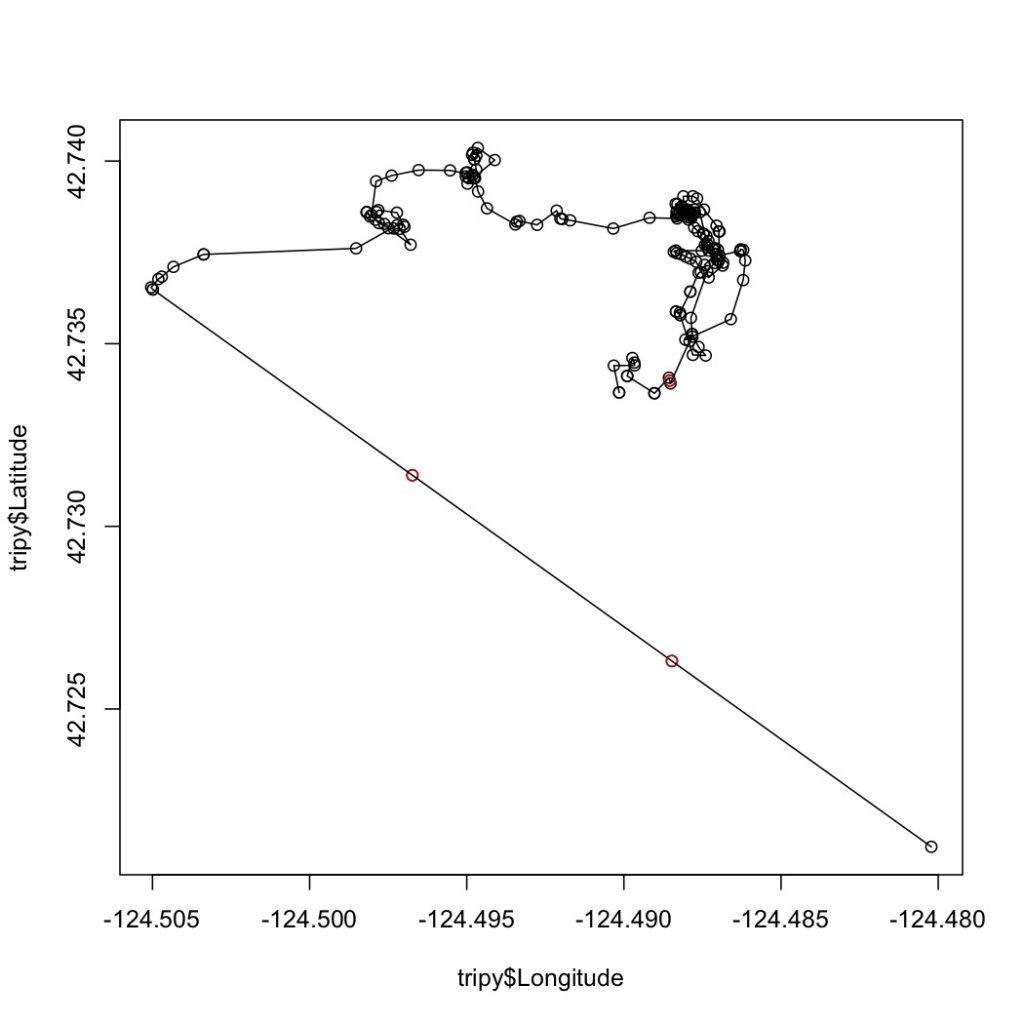
The first step in this process is to run a speed filter over each trackline. The aim of the speed filter is to remove any erroneous points or outliers that must be wrong based on the known travel speeds of gray whales. Barb Lagerquist, a Marine Mammal Institute (MMI) colleague who has tracked gray whales for several field seasons, found that the fastest individual she ever encountered traveled at a speed of 17.3 km/h (personal communication). Therefore, based on this information, my tracklines are run through a speed filter set to remove any points that suggest that the whale traveled at 17.3 km/h or faster (Figure 2).

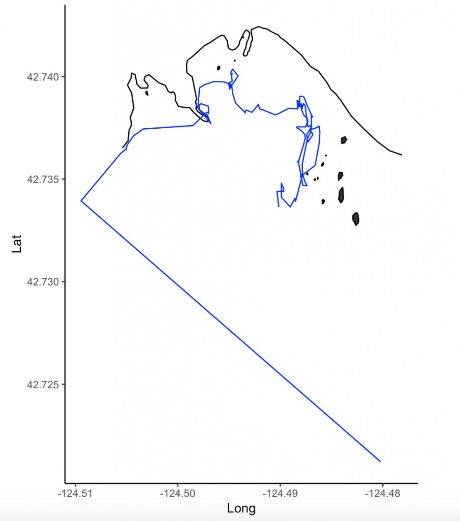
Next, the speed-filtered tracklines are interpolated (Figure 3). Interpolation fills spatial and/or temporal gaps in a data set by evenly spacing points (by distance or time interval) between adjacent points. These gaps sometimes occur in my tracklines when the tracking teams misses one or several surfacings of a whale or because the whale is obscured by a large rock.
After speed filtration and interpolation has occurred, the tracklines are ready to be analyzed using Residence in Space and Time (RST; Torres et al. 2017) to assign behavior state to each location. The questions I am hoping to answer for my thesis are based upon knowing the behavioral state of a whale at a given location and time. In order for me to draw conclusions over whether or not a whale prefers to forage by a reef with kelp rather than a reef without kelp, or whether it prefers Holmesimysis sculpta over Neomysis rayii, I need to know when a whale is actually foraging and when it is not. When we track whales from our cliff site, we assign a behavior to each marked location of an individual. It may sound simple to pick the behavior a whale is currently exhibiting, however it is much harder than it seems. Sometimes the behavioral state of a whale only becomes apparent after tracking it for several minutes. Yet, it’s difficult to change behaviors retroactively while tracking a whale and the qualitative assignment of behavior states is not an objective method. Here is where RST comes in.
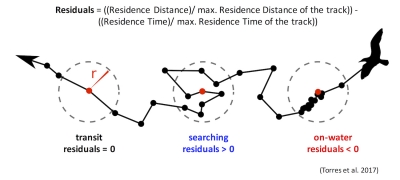
Those of you who have been following the blog for a few years may recall a post written in early 2017 by Rachael Orben, a former post-doc in the GEMM Lab who currently leads the Seabird Oceanography Lab. The post discussed the paper “Classification of Animal Movement Behavior through Residence in Space Time” written by Leigh and Rachael with two other collaborators, which had just been published a few days prior. If you want to know the nitty gritty of what RST is and how it works, I suggest reading Rachael’s blog, the GEMM lab’s brief description of the project and/or the actual paper since it is an open-access publication. However, in a nut shell, RST allows a user to identify three primary behavioral states in a tracking dataset based on the time and distance the individual spent within a given radius. The three behavioral categories are as follows:

- Transit – characterized by short time and distance spent within an area (radius of given size), meaning the individual is traveling.
- Time-intensive – characterized by a long time spent within an area, meaning the individual is spending relatively more time but not moving much distance (such as resting in one spot).
- Time & distance-intensive – characterized by relatively high time and distances spent within an area, meaning the individual is staying within and moving around a lot in an area, such as searching or foraging.
What behavior these three categories represent depends on the resolution of the data analyzed. Is one point every day for two years? Then the data are unlikely to represent resting. Or is the data 1 point every second for 1 hour? In which case travel segments may cover short distances. On average, my gray whale tracklines are composed of a point every 4-5 minutes for 1-2 hours. Bases on this scale of tracking data, I will interpret the categories as follows: Transit is still travel, time & distance-intensive points represent locations where the whale was searching because it was moving around one area for a while, and time-intensive points represent foraging behavior because the whale has ‘found what it is looking for’ and is spending lots of time there but not moving around much anymore. The great thing about RST is that it removes the bias that is introduced by my field team when assigning behavioral states to individual whales (Figure 5). RST looks at the tracklines in a very objective way and determines the behavioral categories quantitatively, which helps to remove the human subjectivity.
While it took quite a bit of troubleshooting in R and overcoming error messages to make the codes run on my data, I am proud to have results that are interesting and meaningful with which I can now start to answer some of my many research questions. My next steps are to create interpolated prey density and distance to kelp layers in ArcGIS. I will then be able to overlay my cleaned up tracklines to start teasing out potential patterns and relationships between individual whale foraging movements and their environment.
Literature cited
Torres, L. G., R. A. Orben, I. Tolkova, and D. R. Thompson. 2017. Classification of animal movement behavior through residence in space and time. PLoS ONE: doi. org/10.1371/journal.pone.0168513.


Hello! I’ve just discovered this super insightful blog and also the work of your laboratory member recently on PLOS. I am currently working with cow movement data in order to analyze their behavior as well. However as you said in this blog post… there are errors found when I run the R code. I was thinking because the C file is built under 32-bit? (I am not a programming advance so any help is appreciated). Also I am using MacOS and the first error I got is when trying to import the .so image file. Can you provide more information on how to tackle this error? Thanks in advance!