bioinformatics « Center for Quantitative Life Sciences

Bing Wang, CQLS; Marco Corrales Ugalde HMSC; Elena Conser HMSC

By leveraging the scalability and parallelization of high-performance computing (HPC), CQLS and CEOAS Research Computing, collaborated with PhD student Elena Conser and postdoctoral research scholar Marco Corrales Ugalde from Hatfield Marine Science Center’s (HMSC) Plankton Ecology Laboratory to complete the end-to-end processing of 128 TB of plankton image data collected during Winter and Summer of 2022 and 2023 along the Pacific Northwest coast of the United States (Figure 1a) .The workflow, which encompassed image segmentation, training library development, and custom convolutional neural network (CNN) model training, produced taxonomic classification and size data for 11.2 billion plankton and particle images. Processing was performed on the CQLS and CEOAS HPC and Pittsburgh Supercomputing Center Bridges-2, consuming over 40,000 GPU hours and 3 million CPU hours. CQLS and CEOAS Research Computing provided essential high-performance computing resources, such as NVIDIA Hopper GPUs, IBM PowerPC system, and multi-terabyte NFS storage. In addition, these computing centers contributed with software development that expedited the processing of images through our pipeline, such as custom web applications for image visualization and annotation, and automated, high-throughput pipelines for segmentation, classification, and model training.

Project introduction

Plankton (meaning “wanderer,” in Greek) are composed of a diverse community of single-celled and multicellular organisms, comprising an extensive size range from less than 0.1 micrometers to several meters. Planktonic organisms also vary extensively in their taxonomy, from bacteria and protists to the early life stages of fishes and crustaceans. The distribution and composition of this diverse “drifting” community is determined in part by the ocean’s currents and chemistry. Marine plankton form the foundation of oceanic food webs and play a vital role in sustaining key ecosystem services, such as climate regulation via the fixation of atmospheric CO₂, the deposition of organic matter to the ocean’s floor, and by the production of biomass at lower levels of the food chain, which sustains global fisheries productivity. Thus, understanding plankton communities is critical for forecasting the impacts of climate change on marine ecosystems and evaluating how these changes may affect climate and global food security.

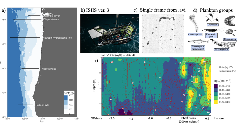
Figure 1. Plankton imagery was collected along several latitudinal transects through the Pacific Northwest coast (a), by the In-situ Ichthyoplankton Imaging System (ISIIS) (b). This data is split into frames (c) and then individual plankton and particle images (d). The high image capture rate (20 frames/second) along a large spatial range allows to provide a detailed description of plankton abundance patterns (colors in panel e) and their relation to oceanographic features (Chlorophyll concentration, dotted isolines, and Temperature, red isolines).

HMCS’s Plankton Ecology Lab, in collaboration with Bellamare engineering, has been the lead developer of the In-situ Ichthyoplankton Imaging System (ISIIS), a state-of-the-art underwater imaging system (Figure 1b) that captures in situ, real-time images of marine plankton (Figures 1c-d). It utilizes a high-resolution line-scanning camera and shadowgraph imaging technology, enabling imaging of up to 162 liters of water per second with a pixel resolution of 55 µm, and detecting particles ranging from 1 mm to 13 cm in size. In addition, ISIIS is outfitted with oceanographic sensors that measure depth, oxygen, salinity, temperature, and other water characteristics. ISIIS is towed behind a research vessel during field deployments. In a single day, a vessel may cover 100 miles while towing ISIIS. ISIIS collects imagery data at a rate of about 10 GB per minute with its paired camera system. A typical two-week deployment produces datasets containing more than one billion particles and approximately 160 hours of imagery, resulting in over 35 TB of raw data. This unprecedented volume of data, together with its high spatial resolution and simultaneous sampling of the environmental context (Figure 1e) allows to address questions of how mesoscale and submesoscale oceanography determine plankton distribution and food web interactions.

Processing this vast amount of data is complex and highly demanding on computing resources. To address this challenge, CQLS and CEOAS Research Computing developed a comprehensive workflow encompassing image segmentation, training library construction, CNN model development, and large-scale image classification and particle size calculation. In the first step, raw imagery is segmented into smaller regions containing regions of interest. These regions are subsequently classified using a CNN based model (Figure 2). In earlier work, a custom sparse CNN model was developed for classification, but thanks to significant advances in computer vision, more efficient models such as YOLO (“You Only Look Once”) have been developed. To train a new YOLO plankton model, a training library of 72,000 images across 185 classes was constructed. Additionally, a test library of 360,000 images was curated to verify model accuracy and ensure robust performance. This improved workflow was applied to 128 TB of ISIIS video data, enabling the classification and size measurement of 11.2 billion images.

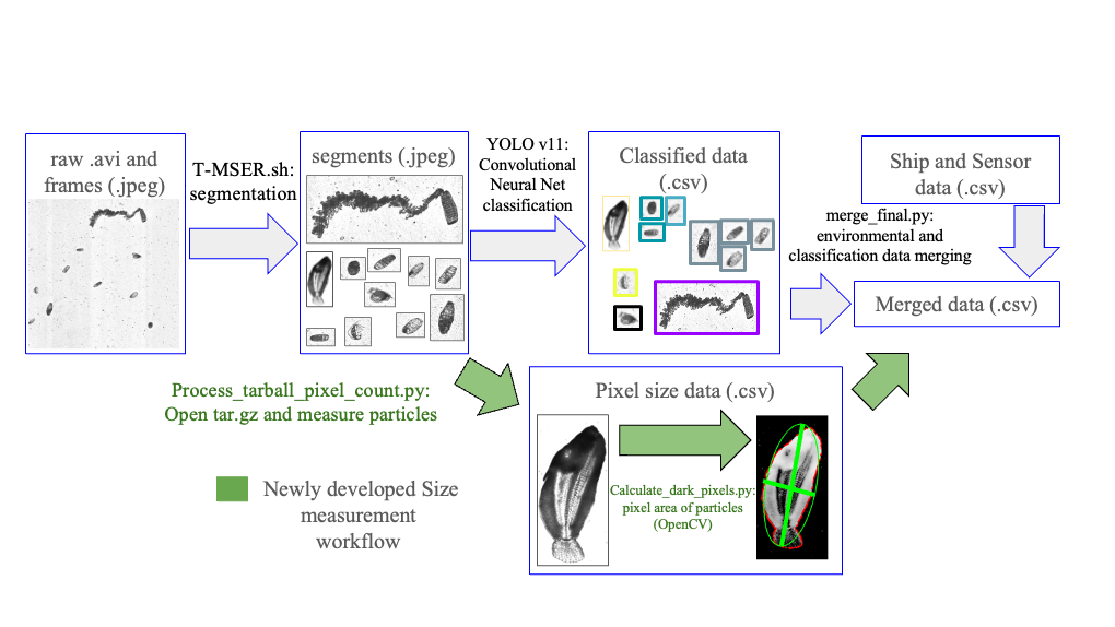
Figure 2. Data processing workflow from raw video to training library development, model training, and plankton classification and particle size estimation

Hardware and software support from CQLS and CEOAS research computing

CQLS and CEOAS Research Computing provide high-performance computing resources for research and is accessible to all OSU research programs. The HPC has a capacity of 9PB for data storage, 45TB of memory, 6500 processing CPUs, and 80+ GPUs. The CQLS and CEOAS HPC can handle more than 20,000 submitted jobs per day.

1. GPU resources

Multiple generations of NVIDIA GPUs are available across architectures on the CQLS and CEOAS HPC, including Tesla V100, Grace Hopper, GTX 1080, and A100, with memory capacities ranging from 11 GB to 480 GB as listed below. GPUs are indispensable for image processing and artificial intelligence, delivering orders of magnitude faster performance than CPUs.

In this project, GPU resources were employed to train YOLO models and to perform classification and particle size estimation of billions of plankton images.

cqls-gpu1 (5 Tesla V100 32GB GPUs), x86 platform
cqls-gpu3 (4 Tesla T4 16GB GPUs), x86 platform
cqls-p9-1 (2 Tesla V100 16GB GPUs), PowerPC platform
cqls-p9-2 (4 Tesla V100 32GB GPUs), PowerPC platform
cqls-p9-3 (4 Tesla V100 16GB GPUs), PowerPC platform
cqls-p9-4 (4 Tesla V100 16GB GPUs), PowerPC platform
ayaya01 (8 GeForce GTX 1080 Ti 11GB GPUs), x86 platform
ayaya02 (8 GeForce GTX 1080 Ti 11GB GPUs), x86 platform
coe-gh01, grace NVIDIA GH200s, 480 GB memory, ARM platform
aerosmith A100, 80GB memory, x86 platform

2. CQLS GitLab

CQLS hosts a GitLab website to streamline project collaboration and code version control for users. https://gitlab.cqls.oregonstate.edu/users/sign_in#ldapprimary

3. Plankton annotator

Plankton Annotator (Figure 3) is a web application developed by Christopher M. Sullivan, Director of CEOAS Research Computing. The tool provides an intuitive platform for the visualization and annotation of plankton imagery. The CQLS and CEOAS Research Computing has the capacity for developing and hosting various web applications. In this project, the Plankton annotator was used to efficiently visualize and annotate plankton images, supporting the creation of reliable training library for downstream YOLO models training.

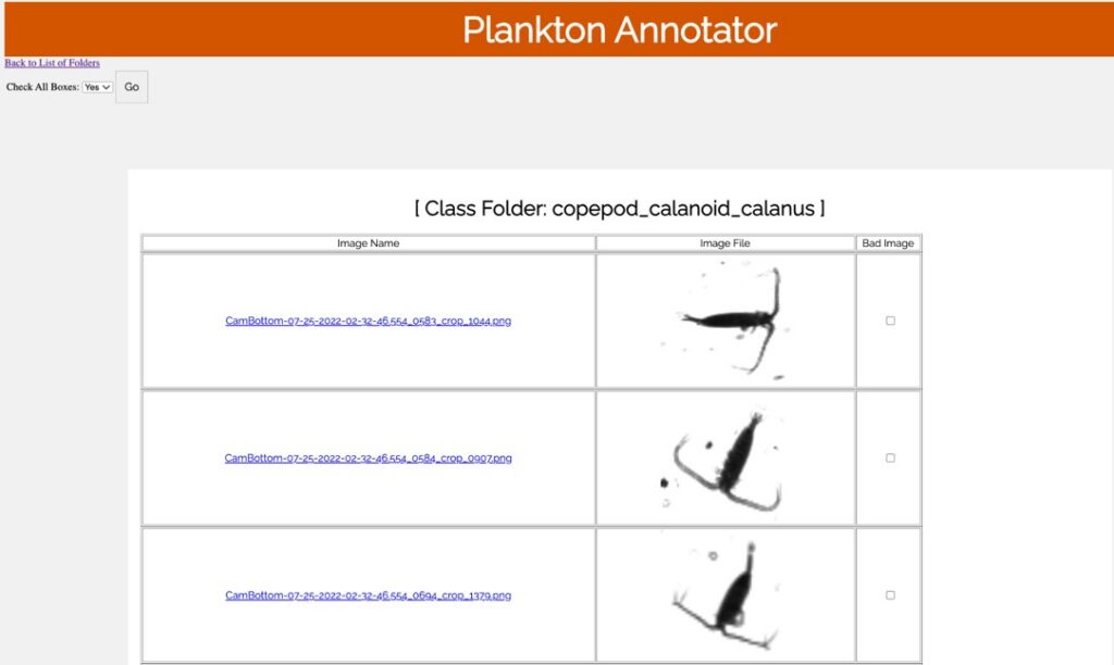
Figure 3. Plankton annotator web application

4. Pipeline developments

CQLS and CEOAS Research Computing has a team of consultants with various programming expertise such as Shell, Python, R, JavaScript, SQL, PHP, and C++. They are available to collaborate on grant proposals, project discussions, experimental design, pipeline development, and data analysis for a wide range of projects in bioinformatics and data science. For this project a series of automated, high-throughput pipelines were updated and created to support image segmentation, model training, species classification and particle size estimation. These pipelines were designed to handle large volumes of data efficiently, ensuring scalability, and reproducibility.

5. Storage

In this project, CQLS and CEOAS HPC provided more than 200 TB of centralized NFS storage to accommodate both raw and processed data. This shared storage infrastructure ensures reliable data access, supports efficient file sharing across the HPC environment, and enables seamless collaboration among researchers.

References

Conser, E. & Corrales Ugalde, M., 2025. The use of high-performance computing in the processing and management of large plankton imaging datasets. [Seminar presentation] Plankton Ecology Laboratory, Hatfield Marine Science Center, Oregon State University, Newport, OR, 19 February.

Schmid, M.S., Daprano, D., Jacobson, K.M., Sullivan, C., Briseño-Avena, C., Luo, J.Y. & Cowen, R.K., 2021. A convolutional neural network based high-throughput image classification pipeline: code and documentation to process plankton underwater imagery using local HPC infrastructure and NSF’s XSEDE. National Aeronautics and Space Administration, Belmont Forum, Extreme Science and Engineering Discovery Environment, vol. 10.

Oregon State University, 2025. Oregon State University Research HPC Documentation. Viewed 18 September 2025, https://docs.hpc.oregonstate.edu.

Ultralytics Inc., 2025. Ultralytics YOLO Docs. Viewed 18 September 2025, https://docs.ultralytics.com.

Sam Talbot, CQLS

High-quality reference genomes are the foundation for much of what our collaborators do at OSU — from mapping reads and calling variants to identifying genes of interest and performing CRISPR knockouts. Obtaining high-quality genomes is still an evolving field: only recently did NIH researchers from the Telomere-to-Telomere consortium bring to full completion a human reference genome; this milestone led to the discovery of nearly 2,000 additional gene predictions, broadly improving our ability to understand genetic variation and epigenetic activity (Sergey Nurk et al. 2022). At the forefront of this achievement was developing protocols for Nanopore ultra-long (UL) sequencing: critical for spanning centromeres, telomeres, and other repeat-rich, heterozygous, and duplicated regions. At CQLS, we’re adapting this methodology for plants to overcome technical biases that persist in traditional short-read and long-read sequencing.

Traditional methods for plant DNA extraction typically rely on aggressive homogenization and lysis methods to break down cell walls, resulting in highly fragmented DNA. Bead beating, vortexing, and even pipette mixing can shear long DNA molecules. By isolating intact nuclei and removing cytoplasmic contaminants without rupturing the nuclear membrane, we can recover DNA fragments that span >60 kilobases to 1Mbp ideal for UL sequencing. We’re pleased to report that our yield of UL reads is on par with other leading institutions.

Figure 1. A. Visualizing of a DNA genome assembly graph (V2) that lacks ultralong reads. Different colors along the graph indicate Simple Bubbles that represent heterozygous loci. The dotted red circle is a Super Bubble composed of many bubbles at different positions within the allelic locus. B. Magnification of the dotted-red circle Super Bubble from a genome assembly that lacks the ultralong reads. C. The same Super Bubble from 1B. identified in the ultralong assembly (V3) shows a significant reduction in the number of bubbles within, vastly reducing complexity of heterozygous calls and read mapping at this allelic locus.

Even modest UL coverage simplifies assemblies and improves accuracy. In benchmarks on a polyploid mint and highly heterozygous hop, ~5x UL depth reduced the total number of spurious short contigs by three-fold compared to genomes without UL support. To illustrate this, Figure 2A. shows a genome assembly graph that lacks UL support. Complex regions in the graph often contain numerous heterozygous loci that exist within a larger heterozygous locus (known as a super bubble). Comparing the same super bubble between two genomes, one without ultralong (Figure 1B) and one with 5x UL coverage (Figure 1C), we can see a significant reduction in total bubbles and complexity. Across the entire genome, UL assemblies reduce super bubbles by ~30% versus no-UL assemblies (Figure 2). These structural improvements carry through to the chromosome validation, yielding cleaner Hi-C contact maps that contain less technical artifacts and stronger assembly metrics overall.

Figure 2. Impact of ultralong reads on raw genome assembly graphs of two plant species.
A polyploid species of mint is represented in orange (raw assembly) and blue (UL reads). Highly heterozygous hop in green (raw assembly) and yellow (UL reads). Plots represent three distinct categories of assembly graph statistics: the number of super bubble, the number of insertions within bubbles and the total number of sequential bubbles.

Ultralong reads deliver biological insights by resolving previously unknown regions that can erroneously impact downstream analysis. Many facets of gene function and regulation have been found to be embedded within or adjacent to transposable-element rich regions that are difficult to assemble correctly without ultralong support. In mint, UL reads led to a nearly seven-fold reduction in an expanded higher-order nucleotide repeat, greatly clarifying our understanding of a centromeric region. We expect UL data to continue strengthening our understanding of biology, especially in non-model species that may hold unknown complexity.

References

Sergey Nurk et al. ,The complete sequence of a human genome.Science376,44-53(2022).DOI:10.1126/science.abj6987

Ed Davis, CQLS

In a collaboration between the Tom Sharpton and Steve Giovannoni labs in the microbiology department, graduate student Seb Singleton designed and performed a study to examine degradation of, and the communities that form biofilms on, plastics in the ocean. Plastic waste accumulation in marine environments is a growing problem that has global effects on the macro and micro scales. In order to understand the ecology surrounding plastic-colonizing bacteria in marine environments, Seb designed a 3 month-long study to examine the changes in biofilm communities as well as structural and chemical changes in the polymer surfaces on high density polyethylene (HDPE), low density polyethylene (LDPE), and polypropylene (PP). An overview of the study design is shown below in Figure 1 from the paper.

Figure 1. Summarized experimental workflow: sample collection (biweekly over 3 months) to downstream analysis [cultivation, 16S (V4) sequence analysis, ATR-FTIR spectral analysis and HIM imaging].

The CQLS, including sequencing using the MiSeq platform in the core lab, as well as bioinformatics consulting done by senior bioinformatics scientist Ed Davis, was integral to the successful outcome of this study. The study encountered several technical roadblocks that were overcome using novel analytical techniques that leveraged the CQLS compute infrastructure. Here is a brief summary of the findings and difficulties overcome:

Initial Dominance: Common marine microbial families such as Alteromonadaceae, Marinomonadaceae, and Vibrionaceae were initially prevalent.
Community Shift: A significant transition in microbial composition occurred between days 42 and 56, with Hyphomonadaceae and Rhodobacteraceae becoming more dominant. These community shifts also coincided with the passing of Tropical Storm Henri!
Rare Taxa: 8,641 colonizing taxa (Amplicon Sequence Variants; ASVs) were identified in total, with 594 overall ASVs enriched on one or more polymer types vs. the glass control, and only 25 ASVs, including known hydrocarbon degraders, significantly enriched on specific plastics.
- Plastic types differ in the ‘rare’ taxa they recruit: Five were specifically enriched on HDPE, nine on LDPE, and eleven on PP.
Taxonomic Assignment Difficulties: Of the 594 significant ASVs, many were unable to be classified to lower taxonomic levels using a classifier trained on the Silva database (i.e. Family and/or Genus level). An alternative classification scheme, called Cladal Taxonomic Annotation (CTA), provided additional taxonomic assignments to 171 (29%) of the significantly enriched ASVs. Most importantly, 8 of the 25 plastic-specific significantly enriched ASVs were better assigned after the CTA.

The shift in taxa over the study period are shown below in Figure 5 from the study:

Figure 5. Gradual temporal shift in a/b diversity shared among material colonizing communities. The Shannon alpha diversity plot (A), Bray-Curtis PCoA (MDS) ordination (B), and Relative abundance stacked bar chart (C) showcase the transition in community complexity and inter-, intra-group similarity over time. In plot (A), alpha diversity measures of the substrate attached communities sharply increases following the mid-experimental transition (between days 42 and 56). Plot (B) explores the compositional dissimilarity of the microbial communities (9,069 unique ASVs) present on the plastics, glass and seawater over the incubation period based on a Bray-Curtis distance matrix. Plot (C) shows the community composition of the top 5% taxa present in each substrate type throughout the incubation period.

Taxa enriched on one or more plastics throughout the study are shown below in Figure 7 from
the paper:

Figure 7. Polymer enriched marine taxa. The Log2foldchange plot showcases NBC classified ASVs that were significantly enriched (adjusted p-value ≤ 0.05) on either one or more polymer types throughout the incubation. The color, size and shape of the data points are associated with the enriched taxon’s class, mean abundance, and substrate preference, respectively. Mean abundance is the average of the sequence depth normalized count values for all included samples, whereas Log2FoldChange is the effect size estimate. All ASVs listed possess >3 log fold differences in abundance compared to glass. Day 42 (and 56 for HDPE) Log2FoldChange data were not included due to loss of sample replicates at the time point, similar rationale was used for Day 14 for all three polymers in respect to the loss of glass control biological replicates.

Degradation of plastics was confirmed using high resolution helium ion microscropy (HIM), and
relevant examples are shown below from Figure 4 of the paper:

Figure 4. Post incubation biodegradation artifacts. HIM images of 77-day incubated polyolefins with biofilm removed in contrast to unexposed controls to exhibit artifacts of biodegradation by colonizing taxa. Marine-incubated LDPE (A) (1–4), HDPE (B) (1–2) and PP (C) (1–2). Unexposed polyolefins: LDPE (A), HDPE (B) and PP (C).

This research highlights the complex interactions between microbes and plastic surfaces in
marine environments, offering insights into the ecological impact of plastic pollution.

Citation: Singleton SL, Davis EW, Arnold HK, Daniels AMY, Brander SM, Parsons RJ, Sharpton
TJ and Giovannoni SJ (2023) Identification of rare microbial colonizers of plastic materials
incubated in a coral reef environment. Front. Microbiol. 14:1259014. doi:
10.3389/fmicb.2023.1259014

Tyler Radniecki, CBEE

Born at the beginning of the COVID-19 pandemic, OSU’s wastewater surveillance efforts, led by Drs. Christine Kelly and Tyler Radniecki (both professors in the School of Chemical, Biological and Environmental Engineering), are still going strong. On-going collaborative efforts include researching how wastewater surveillance can contribute to pandemic resilient cities (National Science Foundation), creating a national wastewater surveillance network for tracking antibiotic resistance genes, bacteria and pharmaceuticals (US Environmental Protection Agency), as well as monitoring state-wide community disease dynamics for SARS-CoV-2, influenza and RSV (Oregon Health Authority). Additional current pilot-scale wastewater surveillance projects include monitoring for Candida auris and antibiotic resistance genes at health care facilities and identifying the presence of the markers for H5N1 influenza strain in Oregon communities.

Throughout it all, Oregon State University’s Center of Quantitative Life Sciences (CQLS) has been a critical partner in these efforts. CQLS wet lab staff assist with nucleic acid extractions from wastewater, library preparation and sequencing of wastewater samples. Additionally, CQLS bioinformatics staff have helped develop and implement bioinformatic pipelines to identify wastewater surveillance targets and report relevant results to OHA and the Center for Disease Control and Prevention. I can honestly say that every member of the CQLS staff has played a hand in our wastewater surveillance efforts.

It is due to our collaborative efforts with CQLS that a lot of exciting advancements in wastewater surveillance have been made. For instance, in collaboration with the OSU TRACE team, we demonstrated that wastewater surveillance is less biased than clinical surveillance at estimating COVID-19 prevalence in a community and that wastewater surveillance can identify COVID-19 hotspots and variant compositions of a community. We have used wastewater sequence surveillance to identify COVID-19 variants in a community before they were identified in clinical samples. Additionally, we demonstrated that wastewater sequence surveillance could accurately identify the COVID-19 variant relative abundances in the state, a critical finding as clinical COVID-19 sequencing has declined substantially from its peak. Finally, we have used wastewater surveillance data to help evaluate the effectiveness of COVID-19 policies implemented by Oregon State University during the first two years for the pandemic.

As we continue to move forward with our wastewater surveillance work, the CQLS will remain a critical collaboration. Together we are developing novel bioinformatic tools and pipelines to identify strains of RSV, norovirus and influenza. Additionally, we are moving forward with new wastewater surveillance projects that will explore links between the environment and human pathogens as well as use our national wastewater surveillance network to monitor the spread climate sensitive diseases in the US. While these endeavors remain challenging, I am grateful to have access to the CQLS to advance our goals.

Another great term of the CGRB’s Bioinformatics User Group (BUG) is in the books!

This term we had a wide range of presenters—graduate students to Principle Investigators. It was nice to get the perspective of folks who are in different parts of their careers.

A special thanks to all of our presenters:

Sept 25: Christopher Sullivan and Ken Lett (Center for Genome Research & Biocomputing)

Title: CGRB’s new DFS for one and all!, i.e., Don’t know what a Distributed File System is? Come find out!
Abstract: The CGRB works with researchers to provide the most robust computational infrastructure available today. Many group rely on file services at the heart of their research computing needs and the CGRB has worked for over 2 decades to provide redundant high speed file services. Over the years users have grown to expect the best solution at a very cheap price. Because of this model the CGRB spends a great deal of time evaluating the available systems to ensure we always have the best at the lowest price. In the past year the CGRB has worked to evaluate and purchase new file service hardware that will replace our existing setups. We will be explaining the pathway taken to bring the new service online and some of the new exciting features.

Oct 9: Lillian Padgitt-Cobb (David Hendrix Lab, Biochemistry & Biophysics)

Title: A phased, diploid assembly of the hop (Humulus lupulus) genome reveals patterns of selection and haplotype variation, i.e., Resolving functional and evolutionary mysteries of a large, complex plant genome with genomic data science
Abstract: Hop (Humulus lupulus) is a plant valued for its use in brewing and traditional medicine. Efforts to determine how biosynthetic pathways in hop are regulated have been challenged by its complex genomic landscape. The diploid hop genome is large, repetitive, and heterozygous, which challenged early attempts at sequencing with short-reads. Advances in long-read sequencing have improved detection of repeats and heterozygous regions, revealing that the genome is nearly 78% repetitive. For our assembly, PacBio long-read sequences were assembled with FALCON and phased into haplotype assemblies with FALCON-Unzip. Using the phased, diploid assembly to assess haplotype variation, we discovered genes under positive selection enriched for stress-response, growth, and flowering functions. Comparative analysis of haplotypes provides insight into large-scale structural variation and the selective pressures that have driven hop evolution. The approaches we developed to analyze the phased, diploid assembly of hop have broader applicability to the study of other large, complex genomes.
Lillian’s GitHub: https://github.com/padgittl/CascadeHopAssembly
Hop Genome Browser: http://hopbase.org/

Oct 23: Kelly Vining (Kelly Vining Lab, Horticulture)

Title: R/qtl, i.e., Applications and methods for analysis of quantitative traits
Abstract: R/qtl is an R package that is used for genetic mapping and marker-trait association. This presentation will explore specific features of R/qtl applied to plant breeding populations. Data types, functions, and interpretation of results will be explored.

Nov 6: Ed Davis (Center for Genome Research & Biocomputing)

Title: Introductory microbiome analysis using phyloseq, i.e., How to generate exploratory diversity plots and what they mean
Abstract: Generating high quality, publication ready figures for a microbiome study can be somewhat difficult. An understanding of both the statistical tests and how to effectively use R to produce figures is required, so the learning curve can be somewhat steep. Fortunately, there are several easy-to-use packages in R that facilitate the analysis of microbiome studies using 16S amplicon data, including the phyloseq package that will be the focus of my talk. I will cover the basics of analyzing alpha and beta diversity and provide some code and example images to show how to generate publication ready figures starting from the base phyloseq output. I will also generate some exploratory charts and graphs such that one would be able to form and later test hypotheses using microbiome data. I will be happy to share the examples and code as well, so that I might catalyze the analysis of your own microbiome studies.
Follow up blog post: https://tips.cgrb.oregonstate.edu/posts/phyloseq-bug-meeting-presentation-fall-2019/

Nov 20: Cedar Warman (John Fowler Lab, Botany & Plant Pathology)

Title: High-throughput maize ear phenotyping with a custom-built scanner and machine learning seed detection, i.e., Computer counts corn, correctly.
Abstract: Near-incomprehensible amounts of maize are produced each year, but our understanding of the dominant North American crop is fundamentally incomplete. Of particular interest is the seed-producing structure of maize, the ear. Here, we present a novel maize ear phenotyping system. Our system captures a video of a rotating ear, which is subsequently flattened into a projection of the ear’s surface. Seed positions and genetic markers can be quantified manually from this projection. To increase throughput, we applied deep learning-based computer vision approaches to seed and marker quantification. Our progress towards a completely automated phenotyping system will be described, in addition to challenges we continue to face adapting computer vision technology to maize ears.
Links from Cedar’s presentation:
Movie flattening: github.com/fowler-lab-osu/flatten_all_videos_in_pwd
Seed distribution analysis: github.com/vischulisem/Maize_Scanner
Also here’s a preprint describing the scanner: https://www.biorxiv.org/content/10.1101/780650v2

Dec 4: Christina Mulch (Kelly Vining Lab, Horticulture)

Title: IsoSeq pooling and HiSeq multiplexing comparison for Rubus occidentalis samples to explore Aphid resistance, i.e., Utilizing RNA to find differences between Aphid Resistant and Susceptible plants.
Abstract: Black raspberry (Rubus occidentalis L.) is a small specialty crop produced primarily in the Pacific Northwest of the U.S. A major challenge for its success is Black raspberry necrosis virus vectored by the Large Raspberry Aphid (Amphorophora agathonica A.). We used Pacific Biosciences IsoSeq long read sequencing technology to study the gene expression patterns in leaves following aphid inoculation. We collected samples from a segregating population for resistance to the pest. High quality RNA was extracted from 20 samples, 10 resistant (R) and 10 susceptible (S) using a modified RNA extraction protocol. Data processing was preformed using the IsoSeq3 pipeline. Alignment of each R and S pool to the latest chromosome level black raspberry reference genome used minimap2 according to recommended options for IsoSeq. Reads were filtered based on mapping quality, alignment length, and presence or absence in multiple samples. This study seeks to reveal the genetic underpinning of aphid resistance with the ultimate goal of enabling marker assisted selection.

Thank you for attending and we look forward to seeing you in 2020!

All of the slots for winter 2020 are full, but please contact us if you’re interested in presenting in the future.

The CGRB will be offering three different workshops this fall. For more information and to register, see the CGRB website.

All workshops are available for credit for students or available to non-students as non-credit workshop(s).

To give perspective students a better insight on each course, we’ve conducted short interviews with the instructors about their course.

See course descriptions and the interviews with the instructors below!

Courses Offered:

Introduction to Unix/Linux and Command-Line Data Analysis (2 modules x 5 weeks @ 2 hrs per week)

Instructor: Matthew Peterson

Course Description:

Introduction to Unix/Linux (5 weeks @ 2 hrs per week)

Logistics:
Date & Time: Sep 25 – Oct 23, Mon/Wed 2:00pm – 2:50pm
For credit: BDS599 CRN 20579
Workshop Cost: $250

This module introduces the natural environment of bioinformatics: the Linux command line. Material will cover logging into remote machines, filesystem organization and file manipulation, and installing and using software (including examples such as HMMER, BLAST, and MUSCLE). Finally, we introduce the CGRB research infrastructure (including submitting batch jobs) and concepts for data analysis on the command line with tools such as grep and wc.

Command-Line Data Analysis (5 weeks @ 2 hrs per week)

Logistics:
Date & Time: Nov 4 – Dec 4, Mon/Wed, 2:00pm – 2:50pm
For credit: BDS599 CRN 20580
Workshop Cost: $250

The Linux command-line environment has long been used for analyzing text-based and scientific data, and there are a large number of tools pre-installed for data analysis. These can be chained together to form powerful pipelines. Material will cover these and related tools (including grep, sort, awk, sed, etc.) driven by examples of biological data in a problem-solving context that introduces programmatic thinking. This module also covers regular expressions, a useful syntax for matching and substituting string and sequence data.

Matthew Peterson in the CGRB server room

Q1: What do you hope students gain from this workshop?

My hope is that students come to appreciate the power and flexibility of using the text-based command-line interface to interact with (Linux) computational infrastructures. With practice students will become self-sufficient in utilizing the infrastructure to conduct their own research.

Q2: Favorite topic in your course?

Pipelines! The ability to chain the inputs and outputs of multiple commands to filter data is immensely powerful.

Q3: Who should register for this course?

From the first page of the course syllabus: “Linux/Unix Commands, Bioinformatics Utilities, Computational Infrastructure: If you know nothing about the above, then you are exactly in the right course! WELCOME!”

Q4: Advice for users new to bioinformatics and/or programming?

Practice, practice, practice! Learning how to use the command-line effectively is like making a clay pot, you need to get your hands dirty!

RNA-Sequencing (10 weeks @ 2 hrs per week)

Instructor: Dr. Andrew Black

Course Description:

Logistics:
Date & Time: Sept 25 – Dec 5, Tue/Thur 11:00am – 11:50am
For credit: BDS 599, CRN 20581
Workshop Cost: $500

This course provides an introduction to, and practical experience with, the computational component of bulk-RNA-sequencing. After a general overview, participants will obtain a working introduction to command line, R-studio, and accessing and utilizing a computing infrastructure. Students with then work through a series of exercises cleaning raw FASTQ files, aligning reads to a reference genome, quasi-mapping reads to a transcriptome / de novo assembly, followed by data visualization and Differential Gene Expression analysis.

Dr. Andrew Black will teach the RNA-seq workshop this term.

Q1: What do you hope students gain from this workshop?

I hope that students gain an understanding of the computational workflow involved with RNA-seq and an appreciation of the methodology! My overarching goal with this course is that people can use material from this course as scaffolding for analyzing their own data on the CGRB infrastructure.

Q2: Favorite topic in your course?

I added a lord of the rings theme to my course; students are looking for differentially expressed genes between hobbits and golems. I’m a dork, I know, but I had fun spiking different genes into the data and enjoy having students visualize this.

Q3: Who should register for this course?

Graduate students, postdocs, faculty, or anyone outside of OSU that are interested in receiving an introduction to RNA-seq or for those that are needing to learn the workflow for their own project(s).

Q4: Advice for users new to bioinformatics and/or programming?

Take it one step at a time and get comfortable with several commands before expanding your scope. Also, record your commands / code in a text document, because if you aren’t using it on a daily basis, you’ll forget it!

Data Programming in R (6 weeks @ 3 hrs per week)

Instructor: Dr. Shawn O’Neil

Logistics:
Date & Time: Sept. 25 – Nov. 6, Mon/Weds/Fri 9:00am – 9:50am
For credit: ST 599, CRN 17196
Workshop Cost: $500

The R programming language is widely used for the analysis of statistical data sets. This course introduces the language from a computer science perspective, covering topics such as basic data types (e.g. integers, numerics, characters, vectors, lists, matrices, and data frames), importing and manipulating data (in particular, vector and data-frame indexing), control flow (loops, conditionals, and functions), and good practices for producing readable, reusable, and efficient R code. We’ll also explore functional programming concepts and the powerful data manipulation and visualization packages dplyr and tidyr, and ggplot2.

Q1: What do you hope students gain from this workshop?

I really hope that students gain an appreciation for programming as a creative activity. It’s not just a means to an end, even with a statistical language like R; there’s a lot of room for play and exploration. Simulation, for example, is a great way to explore complex systems and ask ‘what if’ questions. Many languages (including R) support programmatic drawing and data visualization which can be quite fun.

Q2: Favorite topic in your course?

I always enjoy the point when we first start scaling analyses to thousands of statistical tests. It’s an eye-opening moment, and doing so in R introduces ‘functional programming,’ a powerful and increasingly important paradigm for software design.

Q3: Who should register for this course?

Anyone who is interested in doing data analysis, especially of a statistical sort. For those interested in learning programming in a broader sense, our winter Intro to Python series is an excellent overview of fundamental concepts. Although we cover the same topics in the R course, R organizes its features differently than most mainstream programming languages like Python, Java, and C++. Learning both Python and R provides a solid foundation for data science!

Q4: Advice for users new to bioinformatics and/or programming?

I do recommend learning more than one programming language, eventually, as this helps separate deeper concepts from syntax. Find what motivates you and explore it via programming — this could be your primary research project, some field you’ve been wanting to learn more about, or even a hobby.

This blog post was originally published on September 10, 2018 and written by Christopher M. Sullivan, Assistant Director for Biocomputing. Read the whole article here.

The Oregon State University’s Center for Genome Research and Biocomputing (CGRB) and the Plankton Ecology Lab at OSU Hatfield have been collaborating in implementing an image processing pipeline to automate the classification of in situ images of plankton: microscopic organisms at the base of the food web in the world’s oceans and freshwater ecosystems. The imagery collection from a 10-day cruise typically contains approximately 80 TB worth of video, which, in some cases, may convert into image data yielding several billions of segments representing individual plankton and particles that need to be identified; a near impossible task to carry out manually by human experts. While we have a fully functional Convolutional Neural Net (CNN) algorithm that does an excellent job at predicting the identity of the plankton organisms or particles, we have been limited by GPU computational capabilities. We started working with PCI bus based Tesla K40 and K80 GPUs, which were good enough to manage millions of segments. However, when it came to billions of segments, it became a near insurmountable challenge.

R’s default print function for data frames and matrices is not an effective way to display the contents, especially in a html report. RStudio created a R package, DT, that is an interface to the JavaScript library DataTable. DT allows users to have interactive tables that includes searching, sorting, filtering and exporting! I routinely use these tables in my analysis reports.

Install the DT package from cran

First, one must install and load the DT package. Open up RStudio and run the following commands to install and load the DT package:

# Install the DT package
install.packages("DT")
# Load the DT package
library(DT)

Example Table

The print function is not the most effective was to display a table in an HTML R Markdown report.

print(head(mtcars))

This image has an empty alt attribute; its file name is image-10-1024x252.png

Now let’s look at the datatable function for comparison. The input to the datatable function is a data frame or matrix. Let’s make a table with the preloaded iris data that’s in a data.frame. The basic call is DT::datatable(iris) but in our example I’ve added the filter option to the top of the table, and limited the number of entries to 5 per table. See code and table features below:

datatable(iris, filter = "top", 
          options = list(pageLength = 5))

A screen shot of the output looks like:

This image has an empty alt attribute; its file name is image-1024x490.png

Already, the readability is much better than the base r function print. This is a JavaScript based table, stored in a HTML widget, so a flat image doesn’t convey all of the interactive features.

Features

NUMBER OF ENTRIES TO DISPLAY

You’ll notice that there is a drop down menu that says: “Show 5 entries”. The default is 10, but I specified 5 as default with the code pageLength=5. One may select the number of entries to show by using the drop down menu like so:

This image has an empty alt attribute; its file name is image-1.png

SEARCH BAR

The widget also includes a search bar on the top right corner which can be very useful when interactively exploring data. Note at the bottom of the table it shows you how many entries (rows) were found and are being displayed.

This image has an empty alt attribute; its file name is image-2.png

This image has an empty alt attribute; its file name is image-3-1024x58.png

SORT COLUMNS

Notice that to the right of each column name are two arrows: One may sort by ascending or descending order and the direction of the blue arrow indicates by which direction you sorted the column.

This image has an empty alt attribute; its file name is image-6.png

FILTER COLUMNS

The datatable function also allows users to filter each column depending on the datatype: filter numeric columns with a slider & filter columns of class factor with a drop down menu. One must add the filter = "top" (or bottom, etc.) to the code to enable this feature.

This image has an empty alt attribute; its file name is image-7.png — Numeric columns have sliders

This image has an empty alt attribute; its file name is image-8.png — Columns of class factor have a drop down menu

Export Data

Another useful aspect of the datatable function is the “Buttons” extension. This enables users to copy the table, save as a csv, excel or PDF file, or print the table. The table “remembers” what you’ve changed so far—so if you sort by Sepal Length, filter pedal width to > 1 and select species “versicolor” the copied/saved table will have these same restrictions.

datatable(iris, 
          extensions = 'Buttons',
          options = list(dom = 'Bfrtip', 
                         buttons = c('copy', 'csv', 'excel', 'pdf', 'print'))

The above code adds “buttons” to the top of the table like so:

This image has an empty alt attribute; its file name is image-9.png

If one clicks “copy”, the table will be copied to your clipboard, “CSV” or “PDF” will save the table to the give file type, and “print” will bring put the table into a print friendly format and will bring up the print dialog box.

Links and Color

One may also have links in their table. Say you made a data frame with links you want to work in your html report. For example: a data frame of variants w/ links to their position in a genome browser. This is done through not escaping content in the table, specifically the column with the links. The links are made with html and must not be escaped to show up. This applies to other html as well; including color. For me, it was confusing that I had to not escape the html columns. Got it completely backwards the first time I tried it. NOTE: > got replaced with “& gt;” (with no spaces) when it is rendered on the blog… Need to find a fix!

# Make dataframe
df.link <- data.frame(school=c("OSU", "UO", "Linfield", "Willamette"), 
                      mascot=c("beavers", "ducks", "wildcats", "bearcats"),
                      website=c('<a href="http://oregonstate.edu/">oregonstate.edu</a>',
                                '<a href="https://www.uoregon.edu/">uoregon.edu</a>',
                                '<a href="https://www.linfield.edu/">linfield.edu</a>',
                                '<a href="https://www.willamette.edu/">willamette.edu</a>'),
                      School_colors=c('<span style="color:orange">orange & black</span>', 
                                        '<span style="color:green">green & yellow</span>', 
                                        '<span style="color:purple">purple and red</span>', 
                                        '<span style="color:red">red and yellow</span>'))

# When the html columns, 3 & 4, are not escaped, it works!
datatable(df.link, escape = c(1,2,3))

This image has an empty alt attribute; its file name is image-11-1024x333.png

Column Visibility

One may also hide columns from visibility and add a button to add the column back interactively. For example, say we have a data frame called sv.all.i.in. We can hide columns 3 and 4, which are long sequences and disrupt the readability of the table, with the following code:

datatable(sv.all.i.in, extensions = 'Buttons',
          options = list(dom = 'Bfrtip', columnDefs = list(list(visible=FALSE, targets=c(3,4))), 
                         buttons = list(I('colvis'),c('copy', 'csv', 'excel', 'pdf', 'print'))))

This image has an empty alt attribute; its file name is image-12.png

Learn More

There are many more useful features that you can add to your datatable! Learn more here: https://rstudio.github.io/DT/

Friday, September 12, 2014

Poster Award Winners

PostDoc/Trainer/Faculty: Venkatesh Moktali, FungiDB: a functional genomic resource for fungal & oomycete organisms
Grad student: Rachael C. Kuintzle, RNA-Seq Reveals Age-Induced Changes in Rhythmicity in Drosophila Transcriptome
Undergrad student: Alvin Yu, Identifying candidate drugs for atherosclerosis prevention or treatment through a systems biology approach to drug repurposing

Program

8:00	Registration & refreshments (Poster & sponsor setup)
9:00	Brett Tyler, Director, CGRB Introduction, CGRB update
9:20	Shawn O’Neil, Adelaide Rhodes and Kelly Vining, CGRB CGRB Bioinformatics Training: We can help!
	Moderator: Thomas Wolpert
9:30	Sheng-Yang He, Michigan State University Bacterial pathogenesis as a probe of plant biology
10:15	Niklaus J. Grünwald, USDA –ARS/Botany & Plant Pathology Inferring pattern and process of emergence in Phytophthora pathogens
10:40	Break (Poster & sponsor setup)
11:10	Ryan Mueller, Microbiology Linking phylogenetic identity and biogeochemical function of uncultivated marine microbes with novel mass spectrometry techniques
	[Joyce Loper introduces C. Whistler]
11:35	Cheryl Whistler, University of New Hampshire Barbarians at the gate: Adaptive evolution of squid-naive Vibrio fischeri to light organ symbiosis
12:20	Lunch (Poster and Sponsor setups / displays)
	Moderator: Siva Kolluri
1:35	Michael Banks, Cooperative Institute for Marine Resource Studies (CIMRS) Enigmas Related to the Ocean Migration of Chinook Salmon
2:00	Justin Sanders, Microbiology Development of a novel vertebrate model for the cosmopolitan parasite, Toxoplasma gondii
2:25	Patrick De Leenheer, Mathematics/Integrative Biology On finding hotspots and sinks in a multipatch malaria model
2:50	Break (Poster and Sponsor setups / displays)
3:15	Prasad Kopparapu, Environmental & Molecular Toxicology Fighting Cancer with its own tools
3:40	William Bisson, Environmental & Molecular Toxicology Computer-aided cancer drug discovery and chemoprevention in the postgenomic era
4:05	Shankar Subramaniam, University of California – San Diego The Impact of “Omics” on Systems Medicine
4:50	Ron Adams, Interim Vice President of Research Closing remarks
5:00	Poster Session/Reception, Sponsor Displays

Sept 25: Christopher Sullivan and Ken Lett (Center for Genome Research & Biocomputing)

Oct 9: Lillian Padgitt-Cobb (David Hendrix Lab, Biochemistry & Biophysics)

Oct 23: Kelly Vining (Kelly Vining Lab, Horticulture)

Nov 6: Ed Davis (Center for Genome Research & Biocomputing)

Nov 20: Cedar Warman (John Fowler Lab, Botany & Plant Pathology)

Dec 4: Christina Mulch (Kelly Vining Lab, Horticulture)

Courses Offered:

Introduction to Unix/Linux and Command-Line Data Analysis (2 modules x 5 weeks @ 2 hrs per week)

Instructor: Matthew Peterson

Course Description:

Introduction to Unix/Linux (5 weeks @ 2 hrs per week)

Command-Line Data Analysis (5 weeks @ 2 hrs per week)

Q1: What do you hope students gain from this workshop?

Q2: Favorite topic in your course?

Q3: Who should register for this course?

Q4: Advice for users new to bioinformatics and/or programming?

RNA-Sequencing (10 weeks @ 2 hrs per week)

Instructor: Dr. Andrew Black

Course Description:

Q1: What do you hope students gain from this workshop?

Q2: Favorite topic in your course?

Q3: Who should register for this course?

Q4: Advice for users new to bioinformatics and/or programming?

Data Programming in R (6 weeks @ 3 hrs per week)

Instructor: Dr. Shawn O’Neil

Q1: What do you hope students gain from this workshop?

Q2: Favorite topic in your course?

Q3: Who should register for this course?

Q4: Advice for users new to bioinformatics and/or programming?

Install the DT package from cran

Example Table

Features

NUMBER OF ENTRIES TO DISPLAY

SEARCH BAR

SORT COLUMNS

FILTER COLUMNS

Export Data

Links and Color

Column Visibility

Learn More

Poster Award Winners

Program

Contact Info