As mentioned in last weeks blog, I’ve been working on some R analysis for the data we received from OSU. Essentially we’re using the nutritional data we receive to look at the differences between our treatments. We have two trials going on at Belle Fiore, a thinning and irrigation trial and a fertilizer and irrigation trial, I am focusing on the fertilizer trial for my report and poster.
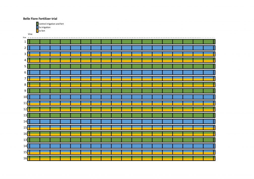
For the fertilizer trial we have four replicates of the four treatment combinations, control irrigation and fertilizer (CC), control irrigation and supplemental fertilizer (CS), supplemental irrigation and control fertilizer (SC), and lastly supplemental irrigation and fertilizer (SS). We use codes as sort of a short annotation, C for control, S for supplemental, and when looking at the code irrigation always comes first. We also use a block design so that if there is variance within the vineyard, for example the west side is dryer than the east, then the blocks or our replicates will keep that from affecting the data. I’ve included a map of the fertilizer treatment below. Rows 1-4 create block 1, rows 5-8 are block 2, rows 9-12 are block 3, and rows 13-16 are block 4.
For the purposes of R analysis we combine the results from each replicate and using R we calculate the least squares means (LS means). We use least squares mean because it minimizes the sum of the squared residuals, meaning it reduces the difference calculated between the observed value and the value produced by the model. This is what helps eliminate any difference between the blocks. We then use those values calculated for each treatment and compare the treatments to see if there is a significant difference between the treatments. The resulting table looks like this:

You’ll notice a letter after each value, the letters just tell us if there is a significant difference between the values. Those that are followed by the same number are not significantly different (P < 0.5). For example in the Manganese (Mn) data for blades CC, CS, and SS are all followed by the letter a so they are not significantly different but, SC is followed by just the letter b which means it is significantly different compared to CC and CS, but not SS because its also followed by the letter b. It’s a little confusing but once you get it, it all makes sense.
We also use R to perform an Analysis of Variance or ANOVA for short. We use a two way ANOVA to study the relationship between our treatment parameters, to see if there is a significant difference between just irrigation and fertilizer and the interaction between the two. The resulting analysis gives us a table of p-values as follows:

In this table I’ve highlighted all the p-values that are significantly different. The interesting thing about comparing the p-values to the LS means is that while according to the p-values a certain treatment may be considered significantly different when looking at the LS means there is no significant difference, for example if you look at Copper (Cu). This is due to the fact that LS means uses a confidence interval to determine significant difference, and sometimes the interval is too large for it to be determined a significant difference. This is why we look at both LS means and p-values, they’re both important and tell us different things about our data.
That was pretty much how I spent my Monday, looking at R outputs and trying to determine what they mean. The rest of the week was pretty normal. On Tuesday I performed a DNA extraction and worked on my report. On Wednesday morning we went out to Belle Fiore and berry sampled, during which we got rained on for like 30 seconds. In the afternoon I got to do an entire juice panel by myself which was pretty cool and honestly didn’t take as long as I thought it would. Then on Thursday we went out to Grestoni and berry sampled, and in the afternoon we took Spad measurements, LICOR photosynthesis analysis, SWP and took the leaves back with us to perform Chlorophyll analysis later.

Hopefully sometime next week I’ll get the second set of data back from OSU so that I can run those numbers through R and compare them to our first set of data. Also if you didn’t get the reference in the title it’s supposed to be a pun/reference to R studio script. Until next time, I hope everyone has a great Labor Day weekend!
