W. Smyth, CEOAS Ocean Mixing Group, Oregon State University
Introduction: The ocean surface

We call the ocean surface an interface because it separates two different types of fluid, air and water. Because of gravity, the denser fluid (water) lies below the lighter fluid (air). Two properties of this interface are important.
1.Exchange. Both water and air cross the interface in small amounts. One result is that sea air tends to be moist (compared to desert air, for example). Likewise, water near the surface tends to be well aerated, with a high oxygen content compared with deeper water.
2.Relative motion. The two fluids are generally in motion relative to one another, the main cause being wind. This motion generates waves (figure 1), and waves greatly accelerate the exchange of fluids across the interface. For example, breaking waves send spray into the air and bubbles into the water. Because both spray droplets and bubbles are small, they are easily absorbed into the surrounding fluid.
The ocean surface is not the only such interface. Similar surfaces are found on lakes and rivers, for example, but more interesting to us are interfaces that exist within the atmosphere and the ocean.
Interfaces in the atmosphere
The atmosphere is composed of air masses with different densities. These air masses tend to arrange themselves into layers, with denser air below and lighter air above. The layers are generally in motion relative to each other, causing wavelike structures and exchange of fluid between the layers, just like at the ocean surface. These internal interfaces are not as sharp as the ocean surface, but we still call them as interfaces because they are much thinner than the layers above and below. Interfaces are usually visible in the afternoon of a partly cloudy day. Typically, a layer of dense air, adjacent to the ground and about a kilometer thick, is overlain by lighter air, and the interface is made visible by clouds. It is often easy to see the relative motion of the layers as the clouds move rapidly relative to the ground. With luck, one can also see the wavelike patterns (figure 2).


Compared with waves at the ocean surface (figure 1), these motions are large and slow. A typical billow is the size of a house, and you have to watch for several minutes to see it change. This is because the difference in density, which causes the wavelike motion, is much smaller than the corresponding difference between air and water at the sea surface. Nonetheless, the motions are similar, and they result in an exchange of air across the interface, with dense air being absorbed into the upper layer and light air absorbed into the lower layer.
Interfaces in the ocean
In seawater, density differences may be caused by differences in either temperature (figure 3) or salinity. For example, temperature differences originate with surface warming in the tropics or cooling in the polar regions. Salinity differences come from river input or from evaporation at the surface (since evaporating water leaves its salt behind).

These cause exchange of fluid between a dense layer (shown in blue) and a light layer (red).
The upshot is that the ocean is arranged into layers just like the atmosphere. These layers move relative to one another due to ocean currents, and water is exchanged across them due to wavelike motions which are, as in the atmosphere, large and slow compared with surface waves.
The exchange of fluids across an interface is an example of mixing. The wavelike motions (like all types of mixing) are turbulent, making their growth and breaking extremely difficult to predict. It is important that we learn to do this, though. For example, suppose that melting of the polar ice caps (figure 4) generates a layer of light, fresh water at the ocean surface in the North Atlantic. This has the potential to slow down ocean currents and thereby radically affect the global climate (as dramatized in the 2004 movie “The Day After Tomorrow”). Another possible outcome, though, is that the light layer of meltwater will mix harmlessly into the underlying ocean. Which will happen? To forecast this, we must predict the rate of mixing across the interface between the light and dense ocean layers.

Other situations where mixing across interfaces is important include:
1. the dispersal of river-borne pollutants into the ocean and
2. El Niño events, which are moderated by the mixing of the sun’s heat into the tropical Pacific ocean.
The wavelike motions described here are called Kelvin-Helmholtz billows. To learn more, see this review article.
Current Research
My students and I study mixing at interfaces mostly using direct numerical simulations on large computers. Figure 5 shows the interface between two layers in motion relative to one another. You’ll see the interface roll up to form two Kelvin-Helmholtz billows (figure 5a). These will merge, develop small-scale instabilities (figure 5b) and ultimately become turbulent (figure 5c, d). Note that, at the end (figure 5d), the interface region is about 10 times thicker than at the beginning (figure 5a). This is the effect of mixing, which we must understand and learn to predict.

To learn more, go to Turbulence Theory and Modeling
The Ocean Mixing Group also makes direct measurements of interfacial mixing in sea-going experiments. Figure 6 shows Kelvin-Helmholtz billows observed in a large (30m) internal wave that was propagating across the continental shelf toward the Oregon coast. Shear within the wave generated the billows much as in figure 5. The red areas at the left are regions where the billows have broken and become turbulent, as in figures 5c and 3.
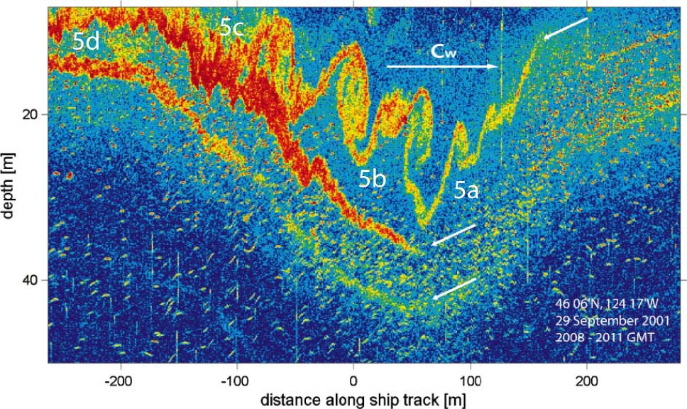
Near the surface the current flows from left to right, the direction of wave propagation, while the underlying fluid flows left to compensate.
The resulting current shear generates the Kelvin-Helmlholtz billows and turbulence. The annotations 5a-5d indicate approximate points where
conditions are comparable to the stages of the DNS shown in figure 5.
For further info, email Bill Smyth.
