06/03/22
Final Project Blog Post and Presentation
1. The research question that you asked (provide one question for each exercise).
- Ex 01: How do offshore wind energy installation locations affect distributions of groundfish, Pacific hake, and northern anchovy along the US West Coast?
- Ex 02:
- How is variable A (sablefish density) affected by variable B (offshore wind energy locations)?
- Then (revised): How does variable A (sablefish population estimates/distributions) change in response to variable B (% of available survey locations)?
- Ex 03: How are the spatial patterns of variable A (sablefish population estimates/distributions) influenced by various spatial scales of B (seafloor bathymetry in this case)?
2. A description of the dataset you examined, with spatial and temporal resolution and extent.
- Ex 01:
- Variable A: groundfish survey data (dark blotched rockfish) from NOAA’s historical survey sites off the coasts of Washington, Oregon, and California which has been gathered consistently over the last 20 years. Temporal resolution/extent is 20 years and the spatial resolution/extent is the whole US West Coast N to S (approx. 50,207 square miles in area).
- Variable B: offshore wind energy installation locations off the coasts of Oregon, and California (Oregon call sites add up to1810 square miles of total area and California wind areas add up to 583 square miles of total area).
- Ex 02:
- Variable A: groundfish survey data (sablefish) from NOAA’s historical survey sites off the coast of Oregon which has been gathered consistently over the last 20 years. Temporal resolution/extent is 20 years and the spatial resolution/extent is the whole US West Coast N to S (approx. 65,816 square miles in area).
- Variable B: offshore wind energy locations off the coast of Oregon (call sites add up to1810 square miles in area).
- Ex 03:
- Variable A: groundfish survey data (sablefish) from NOAA’s historical survey sites off the coast of Oregon which has been gathered consistently over the last 20 years. Temporal resolution/extent is 20 years and the spatial resolution/extent is the whole US West Coast N to S (approx. 65,816 square miles in area).
- Variable B: Bathymetry of the Oregon Coast. Downloaded a NOAA NetCDF file and converted it to a raster file in ArcGIS. I can probably download bathymetry for the whole West Coast on ArcGIS Earth. I couldn’t download the program on the school computers so I will do this at home going forward.
3. Hypotheses: predictions of patterns and processes you looked for.
- Ex 01:
- Groundfish avoid offshore wind energy locations due to unsuitable habitat parameters, intra or interspecies territoriality/competition, lack of appropriate prey species, etc.
- Groundfish are attracted to offshore wind energy locations as they have the potential to function as artificial reefs and attract suitable prey species.
- Ex 02:
- First: What are the relative patterns of sablefish densities within offshore wind energy locations Vs. outside offshore wind energy locations in Oregon.
- Then (revised): What are the relative patterns of Sablefish population estimates/distributions within offshore wind energy locations Vs. outside offshore wind energy locations in Oregon.
- Ex 03: The presence/abundance of sablefish will be positively correlated with deeper oceanic bathymetry on the US West Coast.
4. Approaches: analysis approaches you used.
- Ex 01: Point pattern analysis in ArcGIS Pro of dark blotched rockfish using a 20-year time series of raw survey data that was gathered by NOAA through the agency’s scientific trawl survey efforts on the US West Coast. I exported the Excel data into a table, and then digitized the table into XY points using geoprocessing tools in ArcGIS Pro. I then represented the comparative abundance/distribution of dark blotched rockfish through the use of graduated symbology.
- Ex 02:
- First: Kernel density analysis in ArcGIS Pro of sablefish for the years 1998 and 1999 to understand population densities all along the US West Coast and then within and outside offshore wind energy locations in Oregon.
- Then (revised): Calculation of sablefish population estimate statistics, with standard deviations, as a function of the % of available survey locations through time in ArcGIS Pro. Ended up doing this within offshore wind energy locations Vs. outside of them for the purpose of completing exercise 02 for this class. I will keep working on this methodology going forward.
- Ex 03: A Geographic Weighted Regression in ArcGIS Pro of sablefish population estimates/distributions and Oregon Coast bathymetry.
5. Results: what did you produce — maps? statistical relationships? other? Present the key, important results you created.
- Ex 01:
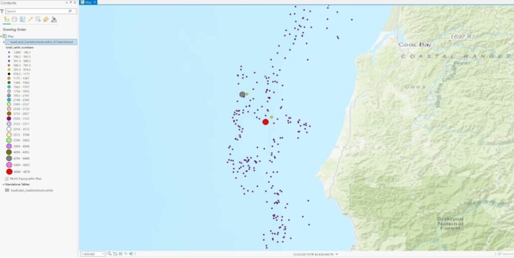
Figure 1. Relative dark blotched rockfish abundances and distributions in Coos Bay, Oregon from 1998 to 2021 (highest abundances are represented by larger symbology).
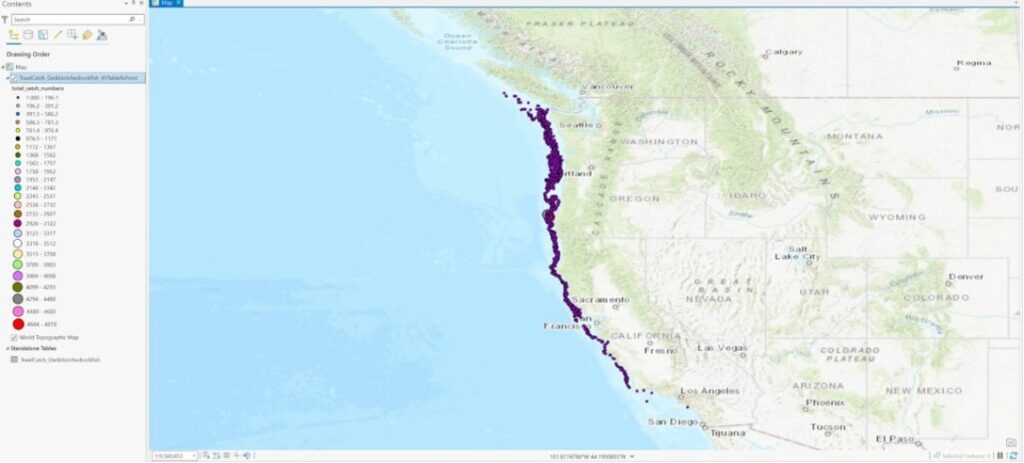
Figure 2. Relative dark blotched rockfish abundances and distributions along the Oregon Coast from 1998 to 2021.
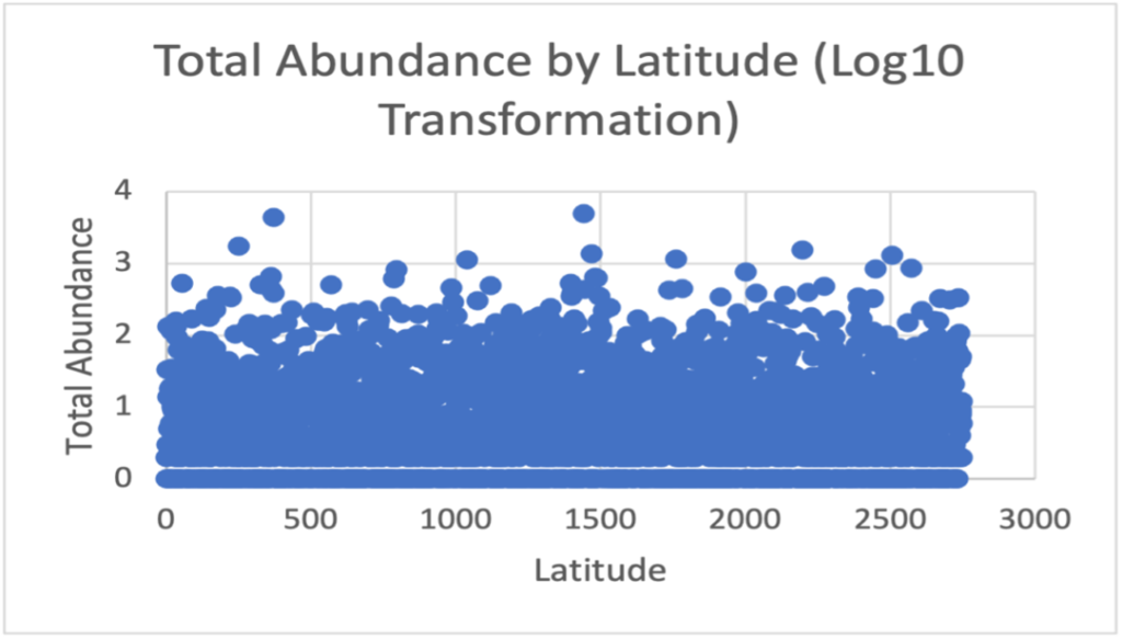
Figure 3. Scatterplot representing a log10 transformation of total abundance of dark blotched rockfish along the Oregon Coast from 1998 to 2021 as a function of latitude location from N to S.
- Ex 02:
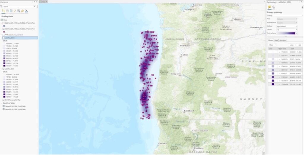
Figure 4. Kernel density map of sablefish off the Oregon Coast in 1998.
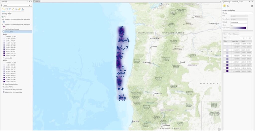
Figure 5. Kernel density map of sablefish off the Oregon Coast in 1999.
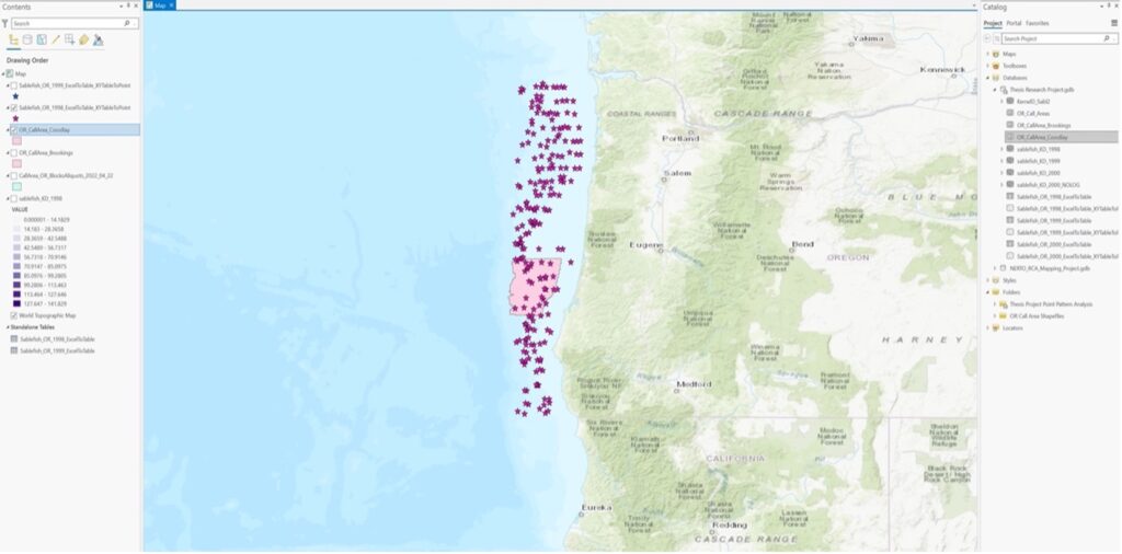
Figure 6. Sablefish population estimates for the year 1998 overlaid upon the Coos Bay call area off the Oregon Coast (need to figure out how to exclude points within the polygon so I can calculate population estimate statistics).
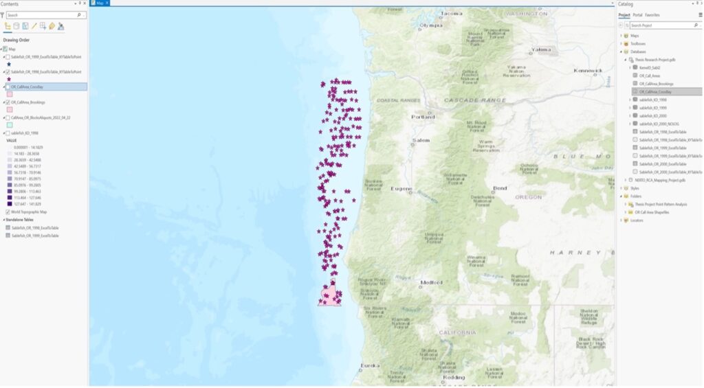
Figure 7. Sablefish population estimates for the year 1998 overlaid upon the Brookings call area off the Oregon Coast (need to figure out how to exclude points within the polygon so I can calculate population estimate statistics).
- Ex 03:
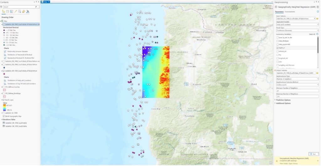
Figure 8. A Geographic Weighted Regression (GWR) map of sablefish population estimates/distributions in 1998 with bathymetry of the Oregon Coast.
6. What did you learn from each of the analyses you conducted (i.e., from each exercise)?
- Ex 01:
- Dark blotched rockfish seem to have an extensive distribution along the US West Coast, from northern WA to southern CA.
- The highest densities of dark blotched rockfish seem to be off the Coast of OR near the Portland area, whereas the highest abundances of dark blotched rockfish in single observations (4684-4878) occurred off the coast of Oregon near Coos Bay, which is very close to one of OR’s proposed offshore wind energy locations.
- Observations of 200-1000 individuals are the most common along the West Coast and these observations occurred in the highest densities.
- There are small gaps in population distributions South of Sacramento, CA. This is the same north of WA but that is not within my study area.
- Ex 02:
- I successfully created kernel density maps of sablefish densities in Oregon for 1998 and 1999. Densities shifted slightly between the two years but overall were quite similar.
- Moderately high densities of sablefish were observed within the Coos Bay offshore wind energy call area as well as within the Brookings offshore wind energy call area, which I think is good.
- I was unable to compute statistics of population estimates with standard deviations within and outside offshore wind polygons as I ran out of time this week. I will keep working on this methodology and work on this analysis going forward.
- Ex 03:
- Sablefish population estimates/distributions were negatively correlated with depth according to the statistics calculated.
- These results do not make sense to me because sablefish distributions should be positively correlated with depth according to the specie’s life history. I think that I did not correctly include the bathymetry raster in this analysis which is why I got negative correlations.
- I tried to use the “extract values to points” geoprocessing tool before rerunning a Geographic Weighted Regression analysis.
- I think I executed the tool correctly, however, the GWR tool failed when I tried to rerun it. I attempted to troubleshoot with the class TA, but we could not figure it out, other than maybe the bathymetry data that I have is too limited. I can try this again once I have downloaded data from ArcGIS Earth which I could not do on the school computers without an admin password. The error message that I got was Geographically Weighted Regression (GWR) failed- “Unable to estimate at least one local model due to multicollinearity (data redundancy)”.
- I can retry this in R or with a different bathymetry dataset going forward.
7. Significance. How are these results important to science and resource managers?
It is vital for the scientific community to gain an understanding of the socioecological impacts of installing and operating OWE off the US West Coast, particularly with regard to NOAA’s fisheries independent biological surveys. These surveys have taken place over many decades and survey designs may have to change in response to OWE operations. Geographic Information Science (GIS) could be a very useful tool for illustrating the impacts to NOAA’s fisheries independent biological surveys by answering research questions in a spatially explicit manner. The analyses that were conducted for this class have informed me about groundfish population estimates and distributions along the US West Coast and how those estimates and distributions may change in response to offshore wind energy development. Ultimately, the approach that I come up with will essentially allow users to calculate how the uncertainty surrounding population estimates will change as a function of the % of area excluded. The tool that I create will function as an optimization approach, to test the sensitivity of surveys to partial surveying.
8. Software learning. Your learning: what did you learn about software (a) Arc-Info, (b) GIS programming in Python, (c) programming in R, (d) Modelbuilder in Arc, or (e) other?
- Arc-Info: nothing.
- GIS programming in Python: I learned some basic Python code from my classmates which I can apply to my own research.
- Programming in R: I learned basic R code from my classmates which I can apply to my own research. I will likely use R a lot going forward.
- Model builder in Arc: not much, however, model builder in ArcGIS Pro may be important for my research going forward as I need to automate my process either in R or ArcGIS Pro.
9. Statistics learning. What did you learn about statistics, including (a) hotspot, (b) spatial autocorrelation (including correlogram, wavelet, Fourier transform/spectral analysis), (c) cross-correlation/regression (cross-correlation, geographically weighted regression [GWR], regression trees, boosted regression trees), (d) multivariate methods (e.g., PCA, multiple component analysis), (e) other techniques (change detection/confusion matrices, other)?
- Hotspot: I did not complete this analysis but I learned a little more about it from my classmates in terms of its applications.
- Spatial autocorrelation: same as above.
- Cross-correlation/regression (Geographic Weighted Regression [GWR]): I conducted a GWR analysis so I learned quite a lot more about it, its applications, and how to interpret its outputs.
- Multivariate methods: I did not complete this analysis but I learned a little more about it from my classmates in terms of its applications.
10. Evolving question. How did the results of each analysis lead you to change/refine your question? Write out the original question you stated at the beginning of the class, and restate the question(s) you now plan to address.
- Ex 01:
- First: How do wind energy installation locations affect current and future distributions of groundfish?
- Then (revised): How do offshore wind energy installation locations affect distributions of groundfish, Pacific hake, and northern anchovy along the US West Coast?
- Ex 02:
- First: How is variable A (sablefish density) affected by variable B (offshore wind energy locations)?
- Then (revised): How does variable A (sablefish population estimates/distributions) change in response to variable B (% of available survey locations)?
- Ex 03: How are the spatial patterns of variable A (sablefish population estimates/distributions) influenced by various spatial scales of B (seafloor bathymetry in this case)?
11. Future techniques. What techniques would you like to explore to answer your research questions in the future?
- Download bathymetry for the whole West Coast on ArcGIS Earth and rerun my GWR analysis in R or ArcGIS Pro.
- Calculate sablefish population estimate statistics, with standard deviations, as a function of the % of available survey locations through time in R or ArcGIS Pro.
- Keep working in R or use Python code/model builder in ArcGIS Pro to automate the process with some kind of four-loop process over the course of the Summer.