Last week, I wrote about forward propagation in a basic neural network. This week, I’m going to cover back propagation and gradient descent. To keep it simple, I’m not going to dive deeply into the math, but I will describe it in very rudimentary terms.
Let’s do a quick recap of forward propagation in training the model. We start with the 3 main layers: the input layer, the hidden layer, and the output layer.
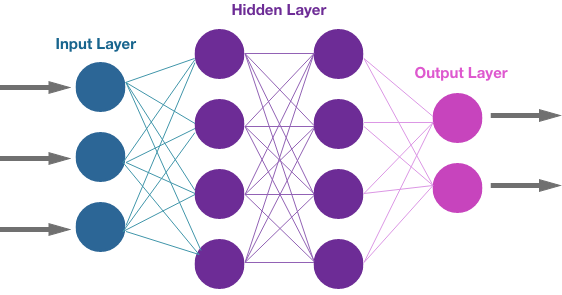
The input layer just takes numerical data as input in the form of a tensor. In the case of an image file, the image is created from a matrix of pixels and each pixel is represented by a color of 3 dimensions (red, green, and blue). Each color in each pixel is encoded as a number between 0 and 255 which determines its strength. A video adds another dimension of time since it is a series of images in a sequential order.
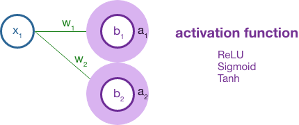
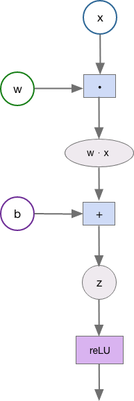
This small network has two hidden layers. Each layer in the hidden layer is associated with an activation function and each neuron in the hidden layer has its own bias (b) assigned randomly at first. The network is connected by weighted edges and each edge is also initially assigned a random weight (w). The fundamental equation between neurons is the dot product of the output from the previous connection (x) and the weight of the edge (w) plus the bias (b).
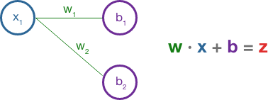
The result here is z, which is fed into the activation function of the neuron. The most common activation function is ReLU which is f(x) = max(0, x). The activation function essentially condenses the tensor, resulting in a more abstract structure as it moves forward in each layer.
Finally, we reach the output layer where we calculate the difference between the current traversal of the network and the expected output (from our labeled training data). Formally, this is calculated by a loss function that might average the squared difference as you would with statistical error.
So, we’ve reached the end of the network and the difference between our current output and the expected output is very high. The labeled picture says “cat” and our current network thinks the image is most likely a “dog”. What do we do now?
Backward propagation and gradient descent to the rescue!
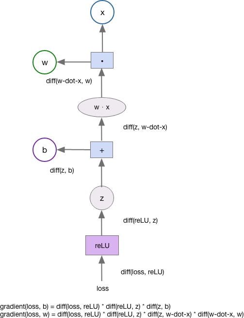
This is an optimization problem and there are two kinds of variables we can change. We can update weights and we can update biases. We want to adjust the weights and biases to get the loss function as close to 0 as possible. We could call the calculations we are using in forward propagation a series of functions. Each of these functions is differentiable; we can take their derivatives to determine the slope at each step along a tensor’s path.
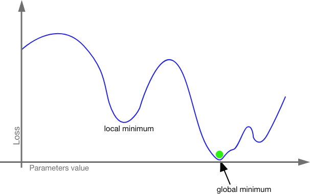
Since we are working with tensors, we combine partial derivatives to determine the gradient (the direction and rate of fastest increase) and then adjust the weights and bias in the opposite direction. The gradient will tell us which weights and biases will have the most impact on the resulting loss. We tweak the weights and biases a lot on those edges and neurons that will have the most impact and we tweak the weights and biases a little for those edges and neurons that will have a little impact. Then we run the input through again and check the loss function again. In this way, we work the model closer and closer to zero cost. We are looking for the global minimum.
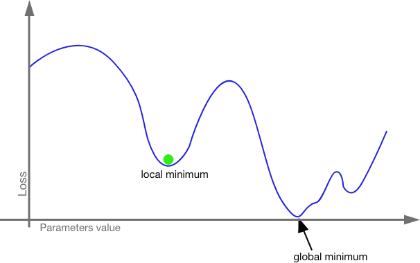
What if we get stuck in a local minimum? This is a real danger. Even traversing a shape of n-dimensional space with thousands or millions of hyper-parameters, it is possible to get caught in a local minimum without realizing it. This is where stochastic gradient descent (SGD) comes in.
With stochastic gradient descent, the model is trained with mini-batches. The entire training set is split up into bite sized batches (usually of about 128 inputs) which are run separately. Each batch is seeded with its own random set of weights and biases. So, even if one batch gets stuck in a local minimum, it is more likely other batches will find the global minimum. The smaller batches also mean that a CPU will not be crushed under the weight of millions of hyper-parameters crunching at once. We can also use momentum here; we can increase the proportion by which we adjust the weights and biases to increase our odds of pushing past local minima.
To find the gradient, we use back propagation. Let’s explore this in a very basic way. As the neural network works forward, it keeps a directed acyclic graph of each operation.

Since each operation is tracked, we can find the derivative of each node with respect to the previous node. We use the chain-rule to determine how each node contributes to the overall loss function.
Because it’s difficult to picture backpropagation and gradient descent using words and static pictures, I’m going to leave you with the beautiful work of Grant Sanderson of 3Blue1Brown who explains the backpropagation of neural networks with the help of his animated pi-gals and pi-guys.
References:
Chollet, F. (November 2021). Deep Learning with Python (2nd edition). Manning Publications. https://learning.oreilly.com/library/view/deep-learning-with/9781617296864/
Sanderson, G. (November 2017). Neural Networks: The basics of neural networks, and the math behind how they learn. 3Blue1Brown. https://www.3blue1brown.com/topics/neural-networks

