For our capstone project, my group is creating a neural network model to classify an audio clip by its musical genre. So, if we are given a 30 second sample of a song, the model should be able to determine if the song is Classical or Hip-Hop or Heavy-Metal. I have written some simple machine learning algorithms before, but three weeks ago, I did not know anything about neural networks. (I also didn’t know anything about audio files.) This week, I am going to go over some of the basics of how a neural network works.
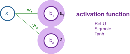
Pictures of neural networks often look like this:

But, what is going on here?
When neural networks are brought up in news articles and tech blogs, they are often compared to biological neural networks. One book I’ve been reading declared this a false comparison and proclaimed that machine learning algorithms are nothing like biological neural networks. Another book suggested that they were, in fact, very much like neural networks. As usual, the truth is somewhere in between.
The concept of machine neural networks was inspired by biological optical neural networks which take in information from the optic nerve (the eye). That visual information is processed in layers of neurons, one after another, which build up pieces of the visual puzzle into the objective world that we see. Like the biological model, a machine neural network model also takes in information and processes it through layers of neurons (or nodes).
A neural network can be divided into 3 layers: the input layer, the hidden layer, and the output layer.
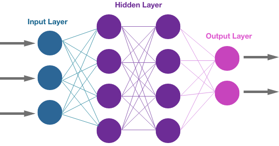
We’ll start with the input layer. This is where the information comes in. The inputs are called tensors.
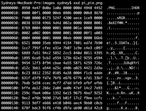
So, what is a tensor? When I started this project, I had heard of TensorFlow, but I didn’t really know what a tensor was. It turns out a tensor is just a data structure that holds our input information. Technically, a tensor is a matrix of N-dimensional space. It sounds very exotic, but you might imagine it as a list of matrices. Or a list of lists of lists. Each tensor will hold data about the object we are looking at. If we are studying an image, the image will be represented by a grid of numerical data.
Here is my Pi a la mode logo image. And here is a section of the numerical grid that represents the grid of pixels that make up the logo. The hexadecimal numbers in the grid define a color for each pixel.

Moving on to the hidden layer.
This is where the math happens that makes a neural network seem like magic. We are going to cover a very basic explanation of forward propagation. Forward propagation is how the information moves from left to right in this diagram.
The basic mathematical building block of the neural network is: x · w + b = z
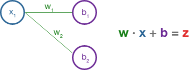
Geometrically, this is known as an affline transformation. In a 2-dimensional space, this might shift a shape object in a way that would still be recognizable. That is, it preserves the points as points, the lines as lines, and their corresponding ratios stay intact. However, angles between the lines may shift and the object may be shifted, rotated, or sheared (tipped to lie in on a different plane). Imagining this in n-dimensional space, requires a higher degree in math (or strong psychedelics).
Let’s take a closer look:
xrepresents the inputswrepresents the weightsbis called the bias
Initially, each weight and each bias is a tensor of random floats set between 0 and 1. The dot between x and w is a dot product between the two tensors.
A quick reminder of dot product product works:
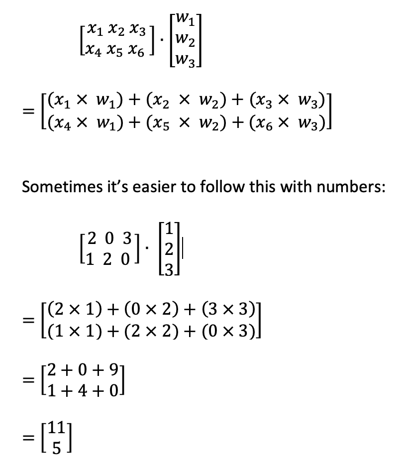
This produces a smaller tensor with fewer dimensions. Now, we add b. It is important to note that the weights and bias will be adjusted as the algorithm progresses.
Once we have calculated x · w + b = z, the result is fed into an activation function.
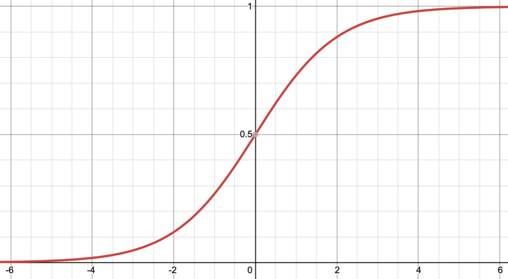
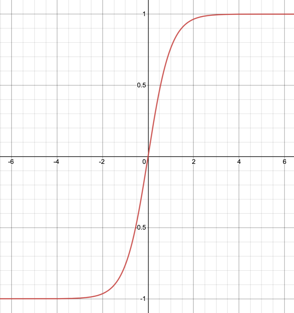
A machine activation function borrows from the activation of a biological neuron as the biological neuron receives input in the form of neurotransmitters that may excite or dampen its own response. In a crude sense, a biological neuron will fire when it reaches a threshold of stimulation from its neighbors. There are 3 common activation functions used in machine neural networks: a sigmoid function, a tanh function, and a ReLU function. Out of these, the ReLU function (Rectified Linear Unit) is generally the most useful. Here is a 2D plot of each:
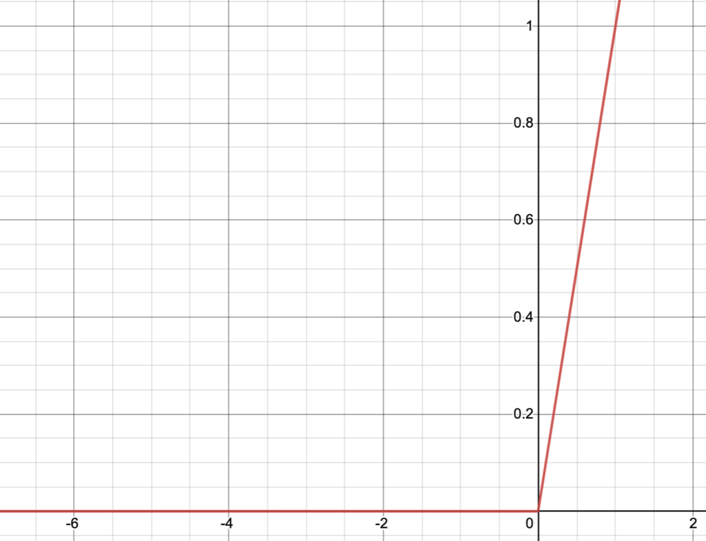
The ReLU function is very simple: f(x) = max(x, 0). It cuts off a geometric object where it reaches zero. Although ReLU is most common, each neuron may have its own activation function.
After the activation function, the result z moves to the next neuron as x, computing the activation function again on x · w + b = z. It moves in the same progression across the hidden layer.
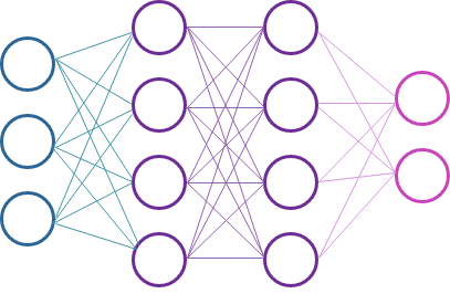
In the picture above, you may notice that all nodes receive input from all nodes in the previous layer. A layer that receives inputs from all nodes in the previous layer is called a Dense layer. There are other ways of designing the connections between nodes, but I’m not far along enough in my reading to cover them here.
Once we’ve traversed the hidden layer, we come to the output layer. At the output layer, we use a loss function to calculate the difference between the expected output and the actual output.
In our genre classification dataset for music audio files, we would probably have the genres indexed into numerical values. If we imagine a list of string values like this:
[ “Classical”, “Folk”, “Hip-Hop”, “Heavy-Metal”, … ]
Classical is at index 0, Folk at index 1, Hip-Hop at index 2, and so on. If we expect the audio file to be classified as Heavy-Metal, the corresponding index should be 3. We would expect the output for this training data to be 3, but say we get 12 instead. The difference between 12 and 3 is 9, so our loss function would return 9.
Now, the neural network algorithm takes the cost (or loss) into consideration and makes adjustments to the weight and bias variables to get an output closer to 3. We want to use the training data to get the loss as close to zero as possible. How do we do this? Through the math-magical marvels of gradient descent and back-propagation. Topics to look forward to in future posts!
References:
Chollet, F. (November 2021). Deep Learning with Python (2nd edition). Manning Publications. https://learning.oreilly.com/library/view/deep-learning-with/9781617296864/
Krohn, J., Beyleveld, G. & Bassens, A. (September 2019). Deep Learning Illustrated: A Visual, Interactive Guide to Artificial Intelligence. Addison-Wesley Professional. https://learning.oreilly.com/library/view/deep-learning-illustrated/9780135116821/
