By Solène Derville, Postdoc, OSU Department of Fisheries and Wildlife, Geospatial Ecology of Marine Megafauna Lab
As a GEMM lab post-doc working on the OPAL project, my main goal for 2021 will be to produce accurate predictive models of baleen whale distribution off the Oregon coast to reduce entanglement risk. For the past months, I have been compiling, cleaning, and processing about two years of data collected by Leigh Torres and Craig Hayslip during monthly repeat surveys conducted onboard United States Coast Guard (USCG) helicopters. These standardized surveys record where and when whales are observed off the Oregon coast. These presence and absence data may now be modeled in relation to habitat, while accounting for effort and detection (as several parameters, such as weather and sea state, can affect the capacity of observers to detect whales at the surface). Considering that several baleen whale species (namely, humpback, fin, blue and gray whales) are known to feed in the area, prey availability is expected to be a major driver of their distribution.
As prey distribution data are frequently the lacking component in the habitat model equation, whale ecologists often resort to using environmental proxies. Variables such as topography (e.g., the depth or slope of the seafloor), water physical and chemical characteristics (e.g., temperature, salinity, oxygen concentration) or ocean circulation (e.g., currents, turbulence) have proved to be good predictors for fish or krill distribution, and in turn potential predictors for whale suitable habitats. In my search for such environmental variables to be tested in our future OPAL models, I have been focusing my research on a fascinating ocean feature: sea height.
Sea height varies both temporally and spatially under the influence of multiple factors, from internal mass of the solid Earth to the orbital revolution of the moon. After reading this blog you will realize that the flatness of the horizon at sea is a deceiving perspective (Figure 1) …

Gravity and the geoid
We all know of Newton’s s discovery of gravity: the attraction force exerted by any object with a given mass on its surroundings. Yet, it is puzzling to think that the rate of acceleration of the apple falling on Newton’s head would have been different if Newton had been anywhere else on Earth.
Why is that and what does it have to do with sea height? On Earth, the standard gravity g is set at 9.80665 m/s2. This constant is called a “standard” because in fact, gravity varies at the surface of our planet, even if estimated at a fixed altitude. Indeed, as gravity is caused by mass, any change in relief or rock composition results in a change in gravity. For instance, magmatic activity in the upper mantle of the Earth and the crust causes a change in rock density and results in a change in gravity measured at the surface.
Gravity therefore is the first reason why the ocean surface is not flat. Gravity shapes an irregular surface called the “geoid”. This hypothetical ocean surface has equal gravitational potential anywhere on Earth and differs from the ellipsoid of reference by as much as 100 m! So to the question whether Earth is round or flat, I would say it is potato shaped (Figure 2)!

The geoid is an essential reference for understanding ocean currents and monitoring changes in sea-level. Hypothetically, if ocean water had equal density everywhere and at any depth, the sea surface should match with the geoid… but that’s not the case. Let’s see why.
Ocean dynamic topography
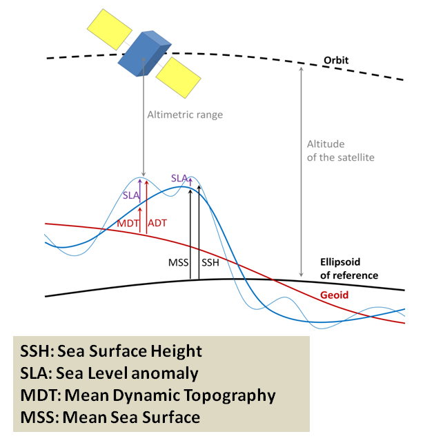
Not unlike the hills and valleys covering landscapes, the ocean surface also has its highs and lows. Except that in the ocean, the surface topography is ever changing. Sea surface height (SSH) measures the average height difference between the observed sea level and the ellipsoid of reference (Figure 3). SSH is mostly affected by ocean circulation and may vary by as much as ±1 m. Indeed, just like the rocks inside the Earth, the water in the ocean varies in density. The vertical and horizontal physical structuring of the ocean was extensively discussed by Dawn last November while she was preparing for her PhD Qualifying Exams. Temperature clearly is at the core of the processes. As thermal expansion increases the space between warming water particles, the volume of a given amount of liquid water increases with increasing temperature. Warmer waters therefore take up “more space” than cooler waters, resulting in an elevated SSH.
SSH may therefore be used as an indicator of oceanographic phenomena such as upwellings, where warm surface waters are replaced by deep, cooler, and nutrient-rich waters moving upwards. The California Current that moves southwards along the North American coast is known as one of the world’s major currents affiliated with strong upwelling zones, which often triggers increased biological productivity. Several studies conducted in the California Current system have found a link between the variations in SSH and whale abundance or foraging activity (Abrahms et al. 2019; Pardo et al. 2015; Becker et al. 2016; Hazen et al. 2016).
SSH is measured by altimeter satellites and is made freely available by the European Space Agency and the US National Aeronautics and Space Administration. Lucky me! Numerous variables are derived from SSH, as shown in Figure 3. Among other things, I was able to download the daily maps of Sea Surface Height Anomaly (SSHa, also referred to as Sea Level Anomaly: SLA) over the Oregon coast from February 2019 to December 2020. SSHa is the difference between observed SSH at a specific time and place from the mean SSH field of reference calculated over a long period of time. Negative values of SSHa potentially suggest upwellings of cooler waters that could be associated with higher prey availability. Figure 4 shows an example of environmental data mining as I try to match SSHa with whale observations made during OPAL surveys. Figure 4B suggests increased whale occurrence where/when SSHa is lower.

and group size (circle size). Monthly averages of SSHa are represented with a colored gradient. B) Monthly averages of SSHa measured over 5-km segments where whales were detected (presence) or not (absence).
Although encouraging, these preliminary insights are just the tip of the modeling iceberg. Many more testing and modeling steps will be required to determine confounding factors and relevant spatio-temporal scales at which these oceanographic variables may be influencing whale distribution off the Oregon coast. I am only at the start of a long road…
References
Abrahms, Briana, Heather Welch, Stephanie Brodie, Michael G. Jacox, Elizabeth A. Becker, Steven J. Bograd, Ladd M. Irvine, Daniel M. Palacios, Bruce R. Mate, and Elliott L. Hazen. 2019. “Dynamic Ensemble Models to Predict Distributions and Anthropogenic Risk Exposure for Highly Mobile Species.” Diversity and Distributions, no. December 2018: 1–12. https://doi.org/10.1111/ddi.12940.
Becker, Elizabeth, Karin Forney, Paul Fiedler, Jay Barlow, Susan Chivers, Christopher Edwards, Andrew Moore, and Jessica Redfern. 2016. “Moving Towards Dynamic Ocean Management: How Well Do Modeled Ocean Products Predict Species Distributions?” Remote Sensing 8 (2): 149. https://doi.org/10.3390/rs8020149.
Hazen, Elliott L, Daniel M Palacios, Karin A Forney, Evan A Howell, Elizabeth Becker, Aimee L Hoover, Ladd Irvine, et al. 2016. “WhaleWatch : A Dynamic Management Tool for Predicting Blue Whale Density in the California Current.” Journal of Applied Ecology 54 (5): 1415–28. https://doi.org/10.1111/1365-2664.12820.
Pardo, Mario A., Tim Gerrodette, Emilio Beier, Diane Gendron, Karin A. Forney, Susan J. Chivers, Jay Barlow, and Daniel M. Palacios. 2015. “Inferring Cetacean Population Densities from the Absolute Dynamic Topography of the Ocean in a Hierarchical Bayesian Framework.” PLOS One 10 (3): 1–23. https://doi.org/10.1371/journal.pone.0120727.
