

I’ve recently found myself (once again) obsessing over the GPU. Specifically, the piece of functionality that modern GPUs have: programmable shaders. The goal of the GPU is to take in data from the CPU – namely data regarding say, a mesh – then run that data through various stages of what’s known as the Graphics Pipeline to ultimately output colors onto your display. Prior to the programmable shader, this pipeline was fixed; meaning developers were quite limited in their ability to fine tune images displayed to their users. While today we’ve been graced by the programmable shaders, there are still pieces of the pipeline that remain fixed. This is actually a good thing. Functionality like primitive assembly, rasterization and per-sample operations are better left to the hardware. If you’ve ever done any graphics programming, you’ve probably seen a diagram that looks like this:
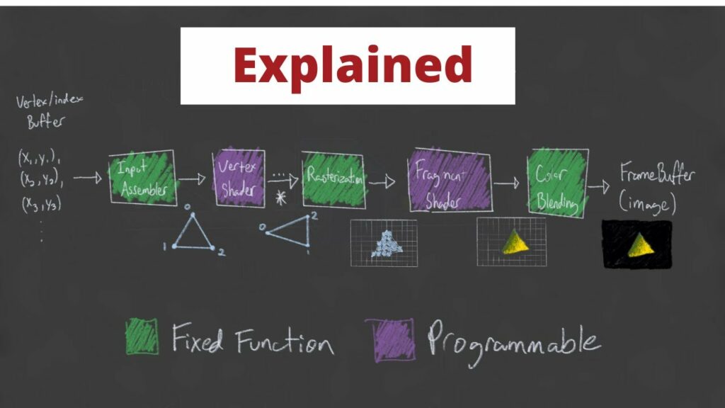
The boxes in green are fixed-function, whereas the purple boxes are programmable. There are actually far more stages than this, but for the most part, these are the stages we’re interested in. And just to be clear, pipeline is a really good name for this as each stage of this process is dependent on the stages prior. The Input Assembly stage is dependent on data being sent to the GPU via the CPU. The Vertex Shader stage is dependent on the input assembler’s triangle/primitive generation so that it can perform any transformations on the vertices that make up each primitive or even perform per-vertex lighting operations. The Rasterization stage needs to figure out what pixels on the screen map to the specified primitives/shapes so data relating to points on the primitives can be interpolated across the primitive, figuring out which of these points are actually within the Camera’s view, calculating depth for perspective cameras and ultimately mapping 3D coordinates to a 2D point on the screen. This leads to the Fragment Shader stage which deals with the fragments generated by the Rasterization Stage; specifically, how each of these pixels should be colored. The final Color Blending stage is responsible for performing any “last-minute” processing on all of the visible pixels using per-pixel shading data from the previous stage, any information that’s context specific to the pipeline state, the current contents of the render target and the contents of the depth and stencil buffers. This final stage also performs depth-testing. This just means that any pixels that are determined to be “behind” another pixel, in other words, will never be seen, will actually be removed when blending occurs. Long story long, the pipeline performs quite a few tasks that are happening unbelievably fast using the power of many, many shader cores and hardware designed to handle these very specific inputs and generate these very specific outputs.
Now, onto our good friend the Compute Shader who doesn’t really belong in the pipeline. As we’ve already seen, the pipelines job is to take data and turn it into colors on your screen. This is all leveraged by the fact that the processors responsible for these operations run in parallel, executing the same (hopefully) operations for every single pixel on the screen. This needs to be fast, especially given the increase in screen resolutions over the past decade. A 4K monitor, 3840 x 2160 pixels, has 8,294,000 pixels! Adding on to this insanity, some of the newer 4K monitors boast a 144Hz refresh rate with a 1ms response time! That’s a lot of work for our GPU to perform! Fortunately, it’s been crafted specifically for this duty. But what if we wanted to use this super-duper parallel computing for other purposes outside of the traditional render-pipeline? Because at the end of the day, the GPU and it’s tons of processors are generally just doing some simple math.
So, if we want to leverage the GPUs parallel processing talents outside of sending a buffer of colors to your monitor, we can use Compute Shaders. Directly from Microsoft, ” A compute shader provides high-speed general purpose computing and takes advantage of the large numbers of parallel processors on the graphics processing unit (GPU). The compute shader provides memory sharing and thread synchronization features to allow more effective parallel programming methods.” What this means is that we can parallelize operations that would otherwise be impractical to run via the CPU (without some of it’s own multi-processing capabilities).
So what might benefit from the use of Compute Shader? Well, some of the more common uses are related to image processing. If you think about the architecture of the GPU as a big grid containing tons of processors, you can think about mapping these processors via their location in the grid. For example, lets say I have a 512 x 512 pixel image where I want to invert every pixel of the original texture and store those inverted values into a new texture. Fortunately, this is a pretty trivial task for a compute shader.
In Unity, the setup code on the CPU looks something like this:
using UnityEngine;

public class ComputeInvertTest : MonoBehaviour
{
    // We want 16 threads per group.
    private const int ThreadsPerGroup = 16;

    // The compute shader.
    [SerializeField] private ComputeShader _testInverter;

    // The texture we want to invert.
    [SerializeField] private Texture2D _sourceTexture;

    // The mesh renderer that we want to apply the inverted texture to.
    [SerializeField] private MeshRenderer _targetMeshRenderer;

    // The texture we're going to store the inverted values for.
    private RenderTexture _writeTexture;

    private void Start()
    {
        // Create the destination texture using the source textures dimensions.
        // Ensure enableRandomWrite is set so we can write to this texture.
        _writeTexture = new RenderTexture(_sourceTexture.width, _sourceTexture.height, 1) {enableRandomWrite = true};

        // Get the resolution of the main texture - in our case, 512 x 512.
        var resolution = new Vector2Int(_sourceTexture.width, _sourceTexture.height);

        // We need to tell the compute shader how many thread groups we want.
        // A good rule of thumb is to figure out how many threads we want per group, then divide
        // the target dimensions by this number.
        // In our case, for our 512 x 512 texture, we want 16 threads per group.
        // This gives us 512 / 16, 512 / 16, or 32 thread groups on both the x and y dimensions.
        var numThreadGroups = resolution / ThreadsPerGroup;

        // Let's find the kernel, or the function, responsible for doing work in the compute shader.
        var inverterKernel = _testInverter.FindKernel("Inverter");

        // Set the texture properties for the source texture and destination textures.
        _testInverter.SetTexture(inverterKernel, Shader.PropertyToID("_WriteTexture"), _writeTexture, 0);
        _testInverter.SetTexture(inverterKernel, Shader.PropertyToID("_ReadTexture"), _sourceTexture, 0);

        // The Dispatch function executes the compute shader using the specified number of thread groups.
        _testInverter.Dispatch(inverterKernel, numThreadGroups.x, numThreadGroups.y, 1);

        // Finally, after the texture has been updated, apply it to the Meshrenderers material.
        _targetMeshRenderer.material.mainTexture = _writeTexture;
    }
}
On the GPU, the code is much simpler.
#pragma kernel Inverter
// The name of the kernel the CPU will look for.
#pragma kernel Inverter

// The number of threads we want per work group - this needs to match what we decided on the CPU side.
static int ThreadsPerGroup = 16;

// The texture we're reading from - no writing allowed here.
Texture2D<float4> _ReadTexture;
// The texture we're writing to, declared as RWTexture2D, or Read/Write Texture2D.
// The <float4> just says that each element in this texture is a 4 component vector, each
// component of type float.
RWTexture2D<float4> _WriteTexture;

// Again, specify the number of threads we want to set per thread group.
[numthreads(ThreadsPerGroup, ThreadsPerGroup, 1)]
void Inverter (uint3 id : SV_DispatchThreadID)
{
    // Write the inverted value to the destination texture.
    _WriteTexture[id.xy] = 1 - _ReadTexture[id.xy];
}
The important bit to realize here is that the attribute above the kernel, [ThreadsPerGroup, ThreadsPerGroup, 1], needs to match the number of threads we set on the CPU side. This value needs to be set at compile time, meaning it can’t change when the program is running. You may also notice this peculiar statement: uint3 id : SV_DispatchThreadID. This is where the magic happens – mapping our threads to our textures. Let’s break down the simple math.
We have a 512 x 512 texture. We want 16 threads per thread-group (or work-group) on both the x and y axes (because our texture is 2D – if our texture was 3D, it would likely be easier to specify 16 on all three axes ) and 1 on the z (we have to have at least 1 thread per group). This SV_DispatchThreadID maps to the following:
SV_GroupID * ThreadsPerGroup + SV_GroupThreadID = SV_DispatchThreadID
This looks like nonsense, I know. The best way to visualize this mapping is, again, like a grid. Taken from Microsoft’s website describing this exact calculation:
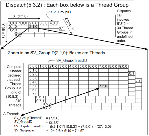
To relate this to our example, let’s remember that our Dispatch call invoked 32 x 32 x 1 Thread groups in an undefined order. So we can think of a 32 x 32 x 1 grid. Each cell of this grid corresponds to another grid – this time mapping to our 16 x 16 x 1 threads per group. This means, if a particular thread has been assigned to say, SV_GroupID of (31, 31, 0), or the last group (as these groups are zero indexed), and it happens to have an SV_GroupdThreadID of (15, 15, 1), or the last thread of this last group, we can calculate it’s 3D id, SV_DispatchThreadID. Doing the math:
SV_GroupID * ThreadsPerGroup + SV_GroupThreadID = SV_DispatchThreadID
(31, 31, 0) * (16, 16, 1) + (15, 15, 1) = (511, 511, 0).
Coincidentally, this is the address, or index, of the last pixel of the texture we’re reading from and writing to! So this mapping worked perfectly. There are a ton of tricks that can be done with playing with threads per group and work group counts, but for this case, it’s pretty straight forward. This is the result:

While this is a pretty contrived example, benchmarking this yielded a grand total of 1ms to invert this 512 x 512 image on the GPU. Just for some perspective, this exact same operation on the CPU took 117ms.
Going even further, using a 4k image, 4096 x 4096 pixels, this is the result:

On the CPU, the inversion took 2,026ms, or just over 2 seconds. On the GPU, the inversion took, once again, 1ms. This is a staggering increase in performance! And just to provide a bit of machine specific information, I have an NVIDIA GeForce GTX 1080 GPU and an Intel Core i7-8700k CPU @ 3.70GHz.
I hope this was an enjoyable read and I hope that you’ve learned something about the wonders of modern technology! And maybe, if you’re a rendering engineer, you’ll consider putting your GPU to work a bit more if you don’t already!
