Month: April 2022

Seeing as how I haven’t done too much in the way of using this platform as a way to write about progress for the Capstone project, I figured now was as good a time as any. My motivation for documenting the development progress of “Virtual Bartender” isn’t because I’m particularly motivated at this moment; nor is it because I’m really leaning into accountability or transparency with the development of this project. I think it’s because I’d like to flesh out some thoughts that generally tend to come up around this point in a somewhat involved project. Specifically, I’ve noticed that I often face an interesting double-edged sword: a truly inspiring, motivating, imaginative state of mind that marks the entry into a project – this tends to be characterized by diagrams, drawings, mind-maps, inspirational art, prototypes, you name it – which is swiftly met with the colder reality that a project almost never meets my unrealistic, imaginative expectations. This often leads me to adding another body to my “dead-projects” folder left to rot somewhere in my C drive.

Alright, enough of the downer negativity! I really don’t want to be a drag, so bear with me here. Because here’s the thing that I’ve realized: all of that day-dreaming about the projects I come to love (and often hate) is ultimately the lifeblood of being a developer, a creator. I guess what I’m getting at is the two are inextricably related. I won’t have motivation for a project if I don’t get inspired – or I need to eat, which is an entirely different topic. However, my inspiration usually comes from an … “out-there” place – movies, music, pictures, dreams, day-dreams, etc. So if my inspiration is born from an imaginary place, which often leads to unrealistic expectations and an inevitable let down, what’s the solution? Well, I certainly don’t have a one-size-fits-all solution, but I’ve slowly been compiling my experiences which have guided me to, at the very least, a bit of awareness and a few tools that tend to help.

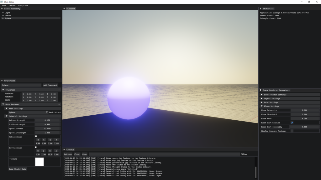
The first tool that comes to mind may be a bit pessimistic at first glance: knowing when your ideas are dumb. Something about the beginning parts of an exciting new project brings an unusual amount of motivation, energy and grandiose ideas! For example, when I started on this Simulation Challenge project, our group opted to do a “bartender” simulation. My initial thought wasn’t, “Let’s give the user the ability to make some simple drinks, let them run around a serve folks”, it was, “I’m going to make a physically realistic simulation of fluid to complement a full-scale realistic bartender simulation with PBR materials and photorealistic graphics!” Of course, this isn’t realistic, but it sure is fun to think about! So the first order of business for me, is to get those ideas out of my system quickly. The best way I can do that is to either sate them, by prototyping those nutty features in a session or two – this is usually just to prove to myself that it’s unrealistic for now – or to really map out everything that would go into implementing them. Again, these are just sobering techniques for the “honeymoon” phase of a project.

The second tool I like to carry around piggy-backs off of the last: breadcrumbs. Somewhere along the way, I go from “Let’s let the user pour fluid with a simple line primitive” to, “Fluid simulation using particles and Laplacian operators”. Now, it isn’t always so easy to remember where I crossed that line separating reality from AAA game feature, so I’ve found it helpful to keep track of my thoughts during this period of early design. The other benefit to keeping track of the thought train that forks off to “Stuck on a feature for weeks”-town is that some of those unrealistic features are really only unrealistic for now. There have been a number of times that I’ve ended up revisiting an idea well into development when it’s been appropriate to either pivot from a current feature or add something fresh. It’s also good to see months into a project that I was at one point really inspired!

The last simple tool that I’m absolutely awful at being consistent with is another really annoying cliché: time management. And I don’t mean, pace-yourself, it’s-a-journey type of management, I mean the you-can’t-allocate-resources-to-save-your-life time management I overestimate certain aspects of a project and underestimate others; I complain about simple, mundane tasks and turn a blind eye to the elephant in the room on a daily basis (refactor that class, seriously, go do it right now!). While I do think there is something to the starving artist trope, I believe there might be something a bit more to the “organized and boring” artist one we don’t often hear about. The times I’ve been the most successful in my short development career have been the times that I’ve been willing to sacrifice time and attention towards the shiny features of my application that I think are cool (they really are, I swear!) to features and tools that have been gasping for air for weeks. There’s also quite a bit to be said about having a semblance of work-life-balance. I have no idea what that is, I just heard that it was valuable.

Ultimately, what I’ve realized is that there’s a beautiful cycle that tends to take place during development that takes longer than a month. Infatuation followed by disinterest, followed by complacency mixed with glimpses of hope, motivation and thoughts of leaving for Mexico, eventually blossoming into the recognition of true progress and the value of hard work, only to be met with more problems to solve, kicking off the cycle anew. But yeah, I’ve been told about that whole work-life-balance thing and how that must fit into that equation somewhere. If you manage to figure out what that looks like, let me know.

In terms of computer graphics, and more prominently, post-processing, bloom is a technique that is used to reproduce a common visual artifact produced by real-world cameras. The effect looks a bit like this:

What we see here is an overwhelmingly bright area on the photo. This is… let’s just say, generally, undesirable – for obvious reasons. However, there are cases where a bit of this flaring effect adds a bit of intensity to points of interest in a scene, or perhaps creating a bit of dramatic contrast. This is also true for real-time (and offline) renders. Too much of this effect oversaturates the image with brightness, defeating the purpose; however, just enough adds some much needed realism in the way we capture the effects of lights in the real-world. And just to be clear, this “Bloom” effect I’m talking about here is a post-processing effect which enhances the relative intensity of the values defining a particular pixels color on the screen based on its relative brightness. That was a bit of a mouthful, so let’s break it down.

First of all, what is a post processing effect? Well, this is from Wikipedia: “The term post-processing (or postproc for short) is used in the video/film business for quality-improvement image processing (specifically digital image processing) methods used in video playback devices, such as stand-alone DVD-Video players; video playing software; and transcoding software. It is also commonly used in real-time 3D rendering (such as in video games) to add additional effects.” TLDR: post processing adds additional effects to the final image of a particular shot, or frame. There are many, many examples of post-processing effects. Just to name a few: Blur, DOF, Bokeh, Bump Mapping, Cel Shading, Film Grain, Dithering, Grayscale, Outlines, Scalines, Shadow Mapping, Vignette, Bloom, Upscaling, Downscaling, Night Vision, Infrared, HDR (High-Dynamic Range) Rendering… I could go on. But this isn’t shocking if you really think about it; how many ways can you potentially alter a picture? Well, your creativity (and your tech) is your only real limitation! All of those filters on your phone? Post-Processing.

Here are a few pictures demonstrating a few commonly seen image effects. No animals were harmed in the making of this blog post – Blue is simply acting as a nice leg rest for my dad.

So now that we have an idea of what Post-Processing effects are and a few common examples, how does one actually apply these effects to images? Well, in a previous blog post, Compute Shaders, I briefly walk through a simple example of utilizing compute shaders to invert the colors of an image. Inversion is a really simple post-processing effect. All we have to do is look at every pixel in the image and subtract it from 1.0. So values that were previously low, perhaps showing a black or grey color, will now look white!

Back to my loveable foot rest:

This picture could be produced in a number of ways – I just happen to be using a compute shader for demoing the inversion of an image, but more common techniques are the use of Vertex/Fragment shaders that work directly in the rendering pipeline. If you want more info on the pipeline, that same post goes through a gentle introduction into the rendering pipeline. To put it simply, whether we’re viewing a picture or a video (a bunch of pictures!), the GPU has sent a 2D grid of pixels to our display. Those 2D pixels are accessible for per-pixel processing within Fragment Shaders. So this is great new for us! Especially if we want to apply these neat effects!

However, if you remember, the rendering pipeline takes a bunch of data about a piece of geometry and works to convert those bits of geometry into triangles that are viewable in 2D screen space so that we can effectively “color” each pixel. And one of the most common usages of the rendering pipeline is for the submission of a mesh. Think about any video game you’ve ever played and think about a character in that game. Whether they exist in 2D or 3D, that character is made up of some very specific geometry (frequently bundled in an object called a Mesh) and the only way that geometry shows up on your screen taking the correct shape, orientation and shading that you’re familiar with is because of that geometric data running through the pipeline. So we can effectively render a mesh by sending it through the pipeline, but how do we apply an effect, say Depth of Field, to every part of our scene that it made into our view? Well, this is where the real magic of post-processing effects come in.

To keep this short, as it could be in its own blog post, the final image we view on our screen is shipped by our GPU in what’s known as a Frame Buffer. This Frame Buffer, often called a Color Buffer, is essentially a 2D grid with the dimensions matching the resolution of your displays dimensions – each cell defining the color of each particular on your display. So, first what we want to do is capture the unfiltered, raw contents of the Frame Buffer that make up the picture we see on screen and store that somewhere. A two-dimensional texture is a pretty intuitive choice due to it’s grid-like nature; not to mention that our GPUs have been optimized to look-up values in a texture, so everyone wins here. Next, we’ll need to take that final image that makes up our scene, then apply our post-processing effects to that. Finally, we can use that filtered texture and map it to a more appropriate mesh, or collection of geometry, for a 2D display. A simple quadrilateral works pretty well here (if you’re viewing this on an 2D screen, you’ll notice that it’s shape is a quadrilateral). And by “map it”, I mean texture mapping, which we won’t get into here. Once the filtered texture has been mapped to our quad, we can simply render that quad every single frame!

After doing quite a bit of work to make my C++ engine render some neat post-processing effects, I learned about the varying complexities involved for a number of techniques. Bloom has got to be one of my favorites! I plan on putting together another post explaining a technique to achieve Bloom in real-time applications – but in the meantime, here are a few very simple photos demoing the effect that I’ve produced in the editor of my work-in-progress game engine!

I’ve recently found myself (once again) obsessing over the GPU. Specifically, the piece of functionality that modern GPUs have: programmable shaders. The goal of the GPU is to take in data from the CPU – namely data regarding say, a mesh – then run that data through various stages of what’s known as the Graphics Pipeline to ultimately output colors onto your display. Prior to the programmable shader, this pipeline was fixed; meaning developers were quite limited in their ability to fine tune images displayed to their users. While today we’ve been graced by the programmable shaders, there are still pieces of the pipeline that remain fixed. This is actually a good thing. Functionality like primitive assembly, rasterization and per-sample operations are better left to the hardware. If you’ve ever done any graphics programming, you’ve probably seen a diagram that looks like this:

The boxes in green are fixed-function, whereas the purple boxes are programmable. There are actually far more stages than this, but for the most part, these are the stages we’re interested in. And just to be clear, pipeline is a really good name for this as each stage of this process is dependent on the stages prior. The Input Assembly stage is dependent on data being sent to the GPU via the CPU. The Vertex Shader stage is dependent on the input assembler’s triangle/primitive generation so that it can perform any transformations on the vertices that make up each primitive or even perform per-vertex lighting operations. The Rasterization stage needs to figure out what pixels on the screen map to the specified primitives/shapes so data relating to points on the primitives can be interpolated across the primitive, figuring out which of these points are actually within the Camera’s view, calculating depth for perspective cameras and ultimately mapping 3D coordinates to a 2D point on the screen. This leads to the Fragment Shader stage which deals with the fragments generated by the Rasterization Stage; specifically, how each of these pixels should be colored. The final Color Blending stage is responsible for performing any “last-minute” processing on all of the visible pixels using per-pixel shading data from the previous stage, any information that’s context specific to the pipeline state, the current contents of the render target and the contents of the depth and stencil buffers. This final stage also performs depth-testing. This just means that any pixels that are determined to be “behind” another pixel, in other words, will never be seen, will actually be removed when blending occurs. Long story long, the pipeline performs quite a few tasks that are happening unbelievably fast using the power of many, many shader cores and hardware designed to handle these very specific inputs and generate these very specific outputs.

Now, onto our good friend the Compute Shader who doesn’t really belong in the pipeline. As we’ve already seen, the pipelines job is to take data and turn it into colors on your screen. This is all leveraged by the fact that the processors responsible for these operations run in parallel, executing the same (hopefully) operations for every single pixel on the screen. This needs to be fast, especially given the increase in screen resolutions over the past decade. A 4K monitor, 3840 x 2160 pixels, has 8,294,000 pixels! Adding on to this insanity, some of the newer 4K monitors boast a 144Hz refresh rate with a 1ms response time! That’s a lot of work for our GPU to perform! Fortunately, it’s been crafted specifically for this duty. But what if we wanted to use this super-duper parallel computing for other purposes outside of the traditional render-pipeline? Because at the end of the day, the GPU and it’s tons of processors are generally just doing some simple math.

So, if we want to leverage the GPUs parallel processing talents outside of sending a buffer of colors to your monitor, we can use Compute Shaders. Directly from Microsoft, ” A compute shader provides high-speed general purpose computing and takes advantage of the large numbers of parallel processors on the graphics processing unit (GPU). The compute shader provides memory sharing and thread synchronization features to allow more effective parallel programming methods.” What this means is that we can parallelize operations that would otherwise be impractical to run via the CPU (without some of it’s own multi-processing capabilities).

So what might benefit from the use of Compute Shader? Well, some of the more common uses are related to image processing. If you think about the architecture of the GPU as a big grid containing tons of processors, you can think about mapping these processors via their location in the grid. For example, lets say I have a 512 x 512 pixel image where I want to invert every pixel of the original texture and store those inverted values into a new texture. Fortunately, this is a pretty trivial task for a compute shader.

In Unity, the setup code on the CPU looks something like this:

using UnityEngine;

public class ComputeInvertTest : MonoBehaviour
{
    // We want 16 threads per group.
    private const int ThreadsPerGroup = 16;
    
    // The compute shader.
    [SerializeField] private ComputeShader _testInverter;
    
    // The texture we want to invert.
    [SerializeField] private Texture2D _sourceTexture;
    
    // The mesh renderer that we want to apply the inverted texture to.
    [SerializeField] private MeshRenderer _targetMeshRenderer;
    
    // The texture we're going to store the inverted values for.
    private RenderTexture _writeTexture;
    
    private void Start()
    {
        // Create the destination texture using the source textures dimensions.
        // Ensure enableRandomWrite is set so we can write to this texture.
        _writeTexture = new RenderTexture(_sourceTexture.width, _sourceTexture.height, 1) {enableRandomWrite = true};

        // Get the resolution of the main texture - in our case, 512 x 512.
        var resolution = new Vector2Int(_sourceTexture.width, _sourceTexture.height);
        
        // We need to tell the compute shader how many thread groups we want.
        // A good rule of thumb is to figure out how many threads we want per group, then divide
        // the target dimensions by this number.
        // In our case, for our 512 x 512 texture, we want 16 threads per group.
        // This gives us 512 / 16, 512 / 16, or 32 thread groups on both the x and y dimensions.
        var numThreadGroups = resolution / ThreadsPerGroup;

        // Let's find the kernel, or the function, responsible for doing work in the compute shader.
        var inverterKernel = _testInverter.FindKernel("Inverter");
        
        // Set the texture properties for the source texture and destination textures.
        _testInverter.SetTexture(inverterKernel, Shader.PropertyToID("_WriteTexture"), _writeTexture, 0);
        _testInverter.SetTexture(inverterKernel, Shader.PropertyToID("_ReadTexture"), _sourceTexture, 0);
        
        // The Dispatch function executes the compute shader using the specified number of thread groups.
        _testInverter.Dispatch(inverterKernel, numThreadGroups.x, numThreadGroups.y, 1);

        // Finally, after the texture has been updated, apply it to the Meshrenderers material.
        _targetMeshRenderer.material.mainTexture = _writeTexture;
    }
}

On the GPU, the code is much simpler.

#pragma kernel Inverter
// The name of the kernel the CPU will look for.
#pragma kernel Inverter

// The number of threads we want per work group - this needs to match what we decided on the CPU side.
static int ThreadsPerGroup = 16;

// The texture we're reading from - no writing allowed here.
Texture2D<float4> _ReadTexture;
// The texture we're writing to, declared as RWTexture2D, or Read/Write Texture2D.
// The <float4> just says that each element in this texture is a 4 component vector, each
// component of type float.
RWTexture2D<float4> _WriteTexture;

// Again, specify the number of threads we want to set per thread group.
[numthreads(ThreadsPerGroup, ThreadsPerGroup, 1)]
void Inverter (uint3 id : SV_DispatchThreadID)
{
    // Write the inverted value to the destination texture.
    _WriteTexture[id.xy] = 1 - _ReadTexture[id.xy]; 
}

The important bit to realize here is that the attribute above the kernel, [ThreadsPerGroup, ThreadsPerGroup, 1], needs to match the number of threads we set on the CPU side. This value needs to be set at compile time, meaning it can’t change when the program is running. You may also notice this peculiar statement: uint3 id : SV_DispatchThreadID. This is where the magic happens – mapping our threads to our textures. Let’s break down the simple math.

We have a 512 x 512 texture. We want 16 threads per thread-group (or work-group) on both the x and y axes (because our texture is 2D – if our texture was 3D, it would likely be easier to specify 16 on all three axes ) and 1 on the z (we have to have at least 1 thread per group). This SV_DispatchThreadID maps to the following:

SV_GroupID * ThreadsPerGroup + SV_GroupThreadID = SV_DispatchThreadID

This looks like nonsense, I know. The best way to visualize this mapping is, again, like a grid. Taken from Microsoft’s website describing this exact calculation:

To relate this to our example, let’s remember that our Dispatch call invoked 32 x 32 x 1 Thread groups in an undefined order. So we can think of a 32 x 32 x 1 grid. Each cell of this grid corresponds to another grid – this time mapping to our 16 x 16 x 1 threads per group. This means, if a particular thread has been assigned to say, SV_GroupID of (31, 31, 0), or the last group (as these groups are zero indexed), and it happens to have an SV_GroupdThreadID of (15, 15, 1), or the last thread of this last group, we can calculate it’s 3D id, SV_DispatchThreadID. Doing the math:

SV_GroupID * ThreadsPerGroup + SV_GroupThreadID = SV_DispatchThreadID

(31, 31, 0) * (16, 16, 1) + (15, 15, 1) = (511, 511, 0).

Coincidentally, this is the address, or index, of the last pixel of the texture we’re reading from and writing to! So this mapping worked perfectly. There are a ton of tricks that can be done with playing with threads per group and work group counts, but for this case, it’s pretty straight forward. This is the result:

While this is a pretty contrived example, benchmarking this yielded a grand total of 1ms to invert this 512 x 512 image on the GPU. Just for some perspective, this exact same operation on the CPU took 117ms.

Going even further, using a 4k image, 4096 x 4096 pixels, this is the result:

On the CPU, the inversion took 2,026ms, or just over 2 seconds. On the GPU, the inversion took, once again, 1ms. This is a staggering increase in performance! And just to provide a bit of machine specific information, I have an NVIDIA GeForce GTX 1080 GPU and an Intel Core i7-8700k CPU @ 3.70GHz.

I hope this was an enjoyable read and I hope that you’ve learned something about the wonders of modern technology! And maybe, if you’re a rendering engineer, you’ll consider putting your GPU to work a bit more if you don’t already!

Every now and then I run into a feature in a project that I can’t help but become totally obsessed with – it’s a bit like a trip to Best Buy or Walmart when the original intent is to buy a phone charger. Half an hour later, your eyes are about as close to the silicon on the new GPU in the electronics section as possible – all the while, your wallet let’s out a puff of smoke reminding you that you’d rather eat this week. While the diehard project manager and realist in me says, “No, no, no, that’s not on the TODO list, that’s good ole fashion scope creep!”, the tech-obsessed junky in me let’s out a rebellious cry, “I don’t care it looks cool!” And in most cases, this is, generally speaking, an unproductive tangent in terms of achieving the original goal. However, in some cases, the time I spend oogling at some new tech, a particular implementation of an algorithm or a new design philosophy actually works to benefit the greater project. And maybe I’m being a bit too black and white, because the reality is, there has yet to be a project that I’m slightly interested in that I haven’t found something that sparks some passion and takes me for an unexpected journey. So, maybe, the two are inextricably connected – it’s difficult for me to truly engage with a project without – in some capacity – getting sucked into a feature that may or may not see the light of day.

This brings us to today’s random, unbelievably time-consuming tangent: fluid simulation. We regret to interrupt your regularly scheduled, Trello-board-approved application development to introduce the world of Navier-Stokes and computational fluid dynamics. Yes, I love simulations. Especially ones where I can really go, “Hm… that actually looks like “insert the real thing here”.” I’ve dabbled with weather simulations and particle simulations, so I figure fluid is next logical step. To put things in a bit of context before I begin my long-winded spiral into drowning the reader with information about fluid simulations (drowning… see what I – I’ll see myself out), this fork in the road originated from my team’s choice of simulation for the Simulation Challenge project for the CS467 Capstone Project.

Out of all of the possible simulations out there, we picked Virtual Bartender. Why? Well, I’m not entirely sure but it sounds pretty fun! I’m used to simulating really, really small stuff or really, really big stuff which isn’t very exciting unless you spent 90% of your childhood building HotWheels tracks. So, the Virtual Bartender gig sounded neat, a nice change of pace and in terms of scope, seemed the most reasonable given the allotted time and our team’s experience using the necessary tools. The tool we’ll be using the most is none other than the Unity game engine. In terms of the simulation itself, the goal is simple – make drinks using tactile, mechanical movements in a VR environment. While this is unbelievably vague, this is as far as we’ve made it so far. We’ve committed ourselves to restricting our focus to ensuring the main mechanic of this simulation, making the dang drinks, feel wonderful. After that, we can choose if the theme is “Space Bar”, or “Under-Sea Atlantis Bar”… or Canada or something… That being said, I don’t have a lot of info regarding the goal of our project, which isn’t a terrible thing at this point in time. We’ve fleshed out the general requirements pertaining to performance, platform/device agnostic API and a general algorithm from which we’ll work to establish the core simulation/gameplay loop. In other words, we have our sand in a truck which we’ll use to build our sand castle – it’s still in the truck, though.

Back to liquids and stuff! You may be two steps ahead of me here, but humor me. We’ve got a Virtual Bar, simulating the experience of a bartender. Now, I’m no bartender and I don’t know the first thing about casual conversation under a dimly lit, stained-glass light fixture from the 80’s while gently swirling a gin and tonic, but I do have a sneaking suspicion there is quite a lot of liquid involved. That being said, how does one simulate liquid? What even is liquid?

Well, to keep things simple, for our purposes, fluid is the volume that defines an infinitesimally small collection of particles that are in constant interaction with one another. And to keep things even simpler so our poor outdated GPUs don’t vomit, maybe we scale back the “infinitesimally” small to “reasonably” small and we partition these particles into their own little cells. Each cell is responsible for keeping track of a bunch of things. Namely, velocity and density. To be even more specific, the cell needs to keep a “memory” of the velocities and densities that it has already recorded. That way, the cell has some knowledge about how it may interact with its neighbors. However, before we get too deep into the meat and potatoes of the core algorithm, it’s worth noting that are a few assumptions we need to make about our fluid. The first is that it’s incompressible. This simply means that the amount of fluid that enters the space stays the same throughout the entire simulation. In other words, conservation of mass. The next is that the means by which the velocities that dictate the circulation of density within the volume is performed via a few processes: diffusion, projection and advection.

Diffusion is the means by which the fluids moves relative to the fluids viscosity, mass of the particles that make up the fluid and temperate (just to name a few variables here).

Projection is the process by which we maintain that first assumption, the incompressible nature of the fluid. After we do some work on the velocities that more or less define the rate of diffusion of the liquid, we need to make sure that we didn’t actually lose any liquid in the process.

Finally, Advection is the means by which the fluid particles themselves move due to the bulk motion of the fluid.

So there seems to be a bit of a niche distinction between Diffusion and Advection, right? Well, the most important difference is that Diffusion refers to a transport mechanism of the fluid that which occurs without any motion of the bulk fluid and Advection refers to the transport mechanism of the fluid due to the motion of the bulk fluid. Still a bit confusing, right? A simple example of Diffusion is the transfer of heat and energy between particles in a drink. A simple example of Advection is the transfer of heat and energy of the particles in the atmosphere as the general circulation of the Earth and regional movements of air around high and low areas of pressure. Diffusion: small. Advection: big.

Back to the general process of simulating fluid: Diffuse the velocities of each cell of the fluid in all axes using the viscosity as the leading factor of change. Perform projection to ensure that the velocities aren’t unreasonable values and that the fluid stays within it’s bounds. Perform advection on each of the cells in all axes using the diffused velocity values as a delta. Again, perform projection to make sure we haven’t broken anything. Finally, we need to diffuse and perform advection on any differing densities – meaning, if we placed dye in water, the dye is the differing density. This final stage is essentially what creates disturbances in the fluid, creating noticeable changes of density throughout the volume.

This was a lot and I’m not quite to the point of implementing this, as there’s just enough math to keep me busy. However, I hope to have a working prototype soon enough that it doesn’t interfere with the development of our Virtual Bar! Worst case scenario, the fluid simulation will never see the light of day and I have a bunch of fun learning about it.