There is something wonderful about time at sea, where your primary obligation is to observe the ocean from sunrise to sunset, day after day, scanning for signs of life. After hours of seemingly empty blue with only an occasional albatross gliding over the swells on broad wings, it is easy to question whether there is life in the expansive, blue, offshore desert. Splashes on the horizon catch your eye, and a group of dolphins rapidly approaches the ship in a flurry of activity. They play in the ship’s bow and wake, leaping out of the swells. Then, just as quickly as they came, they move on. Back to blue, for hours on end… until the next stirring on the horizon. A puff of exhaled air from a whale that first might seem like a whitecap or a smudge of sunscreen or salt spray on your sunglasses. It catches your eye again, and this time you see the dark body and distinctive dorsal fin of a humpback whale.
Figure 1. Pacific white-sided dolphins (Lagenorhynchus obliquidens) play in the big swell and surf the wake of the NOAA ship Bell M. Shimada off Coos Bay, Oregon. Photos: Dawn Barlow.
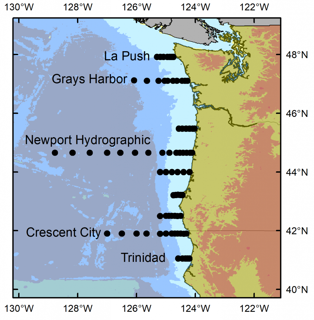
I have just returned from 10 days aboard the NOAA ship Bell M. Shimada, where I was the marine mammal observer on the Northern California Current (NCC) Cruise. These research cruises have sampled the NCC in the winter, spring, and fall for decades. As a result, a wealth of knowledge on the oceanography and plankton community in this dynamic ocean ecosystem has been assimilated by a dedicated team of scientists (find out more via the Newportal Blog). Members of the GEMM Lab have joined this research effort in the past two years, conducting marine mammal surveys during the transits between sampling stations (Fig. 2).
Figure 2. Northern California Current cruise sampling locations, where oceanography and plankton data are collected. Marine mammal surveys were conducted on the transits between stations.
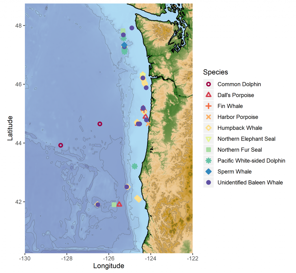
The fall 2019 NCC cruise was a resounding success. We were able to survey a large swath of the ecosystem between Crescent City, CA and La Push, WA, from inshore to 200 miles offshore. During that time, I observed nine different species of marine mammals (Table 1). As often as I use some version of the phrase “the marine environment is patchy and dynamic”, it never fails to sink in a little bit more every time I go to sea. On the map in Fig. 3, note how clustered the marine mammal sightings are. After nearly a full day of observing nothing but blue water, I would find myself scrambling to keep up with recording all the whales and dolphins we were suddenly in the midst of. What drives these clusters of sightings? What is it about the oceanography and prey community that makes any particular area a hotspot for marine mammals? We hope to get at these questions by utilizing the oceanographic data collected throughout the surveys to better understand environmental drivers of these distribution patterns.
Table 1. Summary of marine mammal
sightings from the September 2019 NCC Cruise.
Species
# sightings
Total # individuals
Northern Elephant Seal
1
1
Northern Fur Seal
2
2
Common Dolphin
2
8
Pacific White-sided Dolphin
8
143
Dall’s Porpoise
4
19
Harbor Porpoise
1
3
Sperm Whale
1
1
Fin Whale
1
1
Humpback Whale
22
36
Unidentified Baleen Whale
14
16
Figure 3. Map of marine mammal sighting locations from the September NCC cruise.
It was an auspicious time to survey the Northern California Current. Perhaps you have read recent news reports warning about the formation of another impending marine heatwave, much like the “warm blob” that plagued the North Pacific in 2015. We experienced it first-hand during the NCC cruise, with very warm surface waters off Newport extending out to 200 miles offshore (Fig. 4). A lot of energy input from strong winds would be required to mix that thick, warm layer and allow cool, nutrient-rich water to upwell along the coast. But it is already late September, and as the season shifts from summer to fall we are at the end of our typical upwelling season, and the north winds that would typically drive that mixing are less likely. Time will tell what is in store for the NCC ecosystem as we face the onset of another marine heatwave.
Figure 4. Temperature contours over the upper 150 m from 1-200 miles off Newport, Oregon from Fall 2014-2019. During Fall 2014, the Warm Blob inundated the Oregon shelf. Surface temperatures during that survey were 17°- 18°C along the entire transect. During 2015 and 2016 the warm water (16°C) layer had deepened and occupied the upper 50 m. During 2018, the temperature was 16°C in the upper 20 m and cooler on the shelf, indicative of residual upwelling. During this survey in 2019, we again saw very warm (18°C) temperatures in the upper water column over the entire transect. Image and caption credit: Jennifer Fisher.
It was a joy to spend 10 days at sea with this team of scientists. Insight, collaboration, and innovation are born from interdisciplinary efforts like the NCC cruises. Beyond science, what a privilege it is to be on the ocean with a group of people you can work with and laugh with, from the dock to 200 miles offshore, south to north and back again.
Dawn Barlow on the flying bridge of NOAA Ship Bell M. Shimada, heading out to sea with the Newport bridge in the background. Photo: Anna Bolm.
By: Alexa Kownacki, Ph.D. Student, OSU Department of Fisheries and Wildlife, Geospatial Ecology of Marine Megafauna Lab
Marine mammals are challenging to study for many reasons, and
specifically because they inhabit the areas of the Earth that are uninhabited
by people: the oceans. Monitoring marine mammal populations to gather baselines
on their health condition and reproductive status is not as simple as trap and
release, which is a method often conducted for terrestrial animals. Marine
mammals are constantly moving in vast areas below the surface. Moreover,
cetaceans, which do not spend time on land, are arguably the most challenging
to sample.
One component of my project, based in California, USA, is a health assessment analyzing hormones of the bottlenose dolphins that frequent both the coastal and the offshore waters. Therefore, I am all too familiar with the hurdles of collecting health data from living marine mammals, especially cetaceans. However, the past few decades have seen major advancements in technology both in the laboratory and with equipment, including one tool that continues to be critical in understanding cetacean health: blubber biopsies.
Biopsy dart hitting a bottlenose dolphin below the dorsal fin. Image Source: NMFS
Blubber biopsies are typically obtained via low-powered crossbow with a bumper affixed to the arrow to de-power it once it hits the skin. The arrow tip has a small, pronged metal attachment to collect an eraser-tipped size amount of tissue with surface blubber and skin. I compare this to a skin punch biopsies in humans; it’s small, minimally-invasive, and requires no follow-up care. With a small team of scientists, we use small, rigid-inflatable vessels to survey the known locations of where the bottlenose dolphins tend to gather. Then, we assess the conditions of the seas and of the animals, first making sure we are collecting from animals without potentially lowered immune systems (no large, visible wounds) or calves (less than one years old). Once we have photographed the individual’s dorsal fin to identify the individual, one person assembles the biopsy dart and crossbow apparatus following sterile procedures when attaching the biopsy tips to avoid infection. Another person prepares to photograph the animal to match the biopsy information to the individual dolphin. One scientist aims the crossbow for the body of the dolphin, directly below the dorsal fin, while the another photographs the biopsy dart hitting the animal and watches where it bounces off. Then, the boat maneuvers to the floating biopsy dart to recover the dart and the sample. Finally, the tip with blubber and skin tissue is collected, again using sterile procedures, and the sample is archived for further processing. A similar process, using an air gun instead of a crossbow can be viewed below:
GEMM Lab members using an air gun loaded with a biopsy dart to procure marine mammal blubber from a blue whale in New Zealand. Video Source: GEMM Laboratory.
Part of the biopsy process is holding ourselves to the highest standards in our minimally-invasive technique, which requires constant practice, even on land.
Alexa practicing proper crossbow technique on land under supervision. Image Source: Alexa Kownacki
Blubber is the lipid-rich, vascularized tissue under the
epidermis that is used in thermoregulation and fat storage for marine mammals. Blubber
is an ideal matrix for storing lipophilic (fat-loving) steroid hormones because
of its high fat content. Steroid hormones, such as cortisol, progesterone, and
testosterone, are naturally circulating in the blood stream and are released in
high concentrations during specific events. Unlike blood, blubber is less
dynamic and therefore tells a much longer history of the animal’s nutritional
state, environmental exposure, stress level, and life history status. Blubber
is the cribs-notes version of a marine mammal’s biography over its previous few
months of life. Blood, on the other hand, is the news story from the last 24
hours. Both matrices serve a specific purpose in telling the story, but blubber
is much more feasible to obtain from a cetacean and provides a longer time
frame in terms of information on the past.
A simplified depiction of marine mammal blubber starting from the top (most exterior surface) being the skin surface down to the muscle (most interior). Image Source: schoolnet.org.za
I use blubber biopsies for assessing cortisol, testosterone,
and progesterone in the bottlenose dolphins. Cortisol is a glucocorticoid that
is frequently associated with stress, including in humans. Marine mammals
utilize the same hypothalamic-pituitary-adrenal (HPA) axis that is responsible
for the fight-or-flight response, as well as other metabolic regulations.
During prolonged stressful events, cortisol levels will remain elevated, which
has long-term repercussions for an animal’s health, such as lowered immune
systems and decreased ability to respond to predators. Testosterone and
progesterone are sex hormones, which can be used to indicate sex of the
individual and determine reproductive status. This reproductive information
allows us to assess the population’s composition and structure of males and
females, as well as potential growth or decline in population (West et al.
2014).
Alexa using a crossbow from a small boat off of San Diego, CA. Image Source: Alexa Kownacki
The coastal and offshore bottlenose dolphin ecotypes of interest in my research occupy different locations and are therefore exposed to different health threats. This is a primary reason for conducting health assessments, specifically analyzing blubber hormone levels. The offshore ecotype is found many kilometers offshore and is most often encountered around the southern Channel Islands. In contrast, the coastal ecotype is found within 2 kilometers of shore (Lowther-Thieleking et al. 2015) where they are subjected to more human exposure, both directly and indirectly, because of their close proximity to the mainland of the United States. Coastal dolphins have a higher likelihood of fishery-related mortality, the negative effects of urbanization including coastal runoff and habitat degradation, and recreational activities (Hwang et al. 2014). The blubber hormone data from my project will inform which demographics are most at-risk. From this information, I can provide data supporting why specific resources should be allocated differently and therefore help vulnerable populations. Further proving that the small amount of tissue from a blubber biopsy can help secure a better future for population by adjusting and informing conservation strategies.
Literature Cited:
Hwang, Alice, Richard H Defran, Maddalena Bearzi, Daniela. Maldini, Charles A Saylan, Aime ́e R Lang, Kimberly J Dudzik, Oscar R Guzo n-Zatarain, Dennis L Kelly, and David W Weller. 2014. “Coastal Range and Movements of Common Bottlenose Dolphins (Tursiops Truncatus) off California and Baja California, Mexico.” Bulletin of the Southern California Academy of Sciences 113 (1): 1–13. https://doi.org/10.3390/toxins6010211.
Lowther-Thieleking, Janet L.,
Frederick I. Archer, Aimee R. Lang, and David W. Weller. 2015. “Genetic
Differentiation among Coastal and Offshore Common Bottlenose Dolphins, Tursiops
Truncatus, in the Eastern North Pacific Ocean.” Marine Mammal Science 31
(1): 1–20. https://doi.org/10.1111/mms.12135.
West, Kristi L., Jan Ramer, Janine L. Brown, Jay Sweeney, Erin M. Hanahoe, Tom Reidarson, Jeffry Proudfoot, and Don R. Bergfelt. 2014. “Thyroid Hormone Concentrations in Relation to Age, Sex, Pregnancy, and Perinatal Loss in Bottlenose Dolphins (Tursiops Truncatus).” General and Comparative Endocrinology 197: 73–81. https://doi.org/10.1016/j.ygcen.2013.11.021.
In the GEMM Lab, our research focuses largely on the ecology of marine top predators. Inherent in our work are often assumptions that our study species—wide-ranging predators including whales, dolphins, otters, or seabirds—will distribute themselves relative to their prey. In order to make a living in the highly patchy and dynamic marine environment, predators must find ways to predictably locate and exploit prey resources.
But what about the prey? How do the prey structure themselves relative to their predators? This question is explored in depth in a paper titled “The Landscape of Fear: Ecological Implications of Being Afraid” (Laundre et al. 2010), which we discussed in our most recent lab meeting. When wolves were re-introduced in Yellowstone, the elk increased their vigilance and altered their grazing patterns. As a result, the plant community was altered to reflect this “landscape of fear” that the elk move through, where their distribution not only reflected opportunities for the elk to eat but also the risk of being eaten.
Translating the landscape of fear concept to the marine environment is tricky, but a fascinating exercise in ecological theory. We grappled with drawing parallels between the example system of wolves, elk, and vegetation and baleen whales, zooplankton, and phytoplankton. Relative to grazing mammals like elk, the cognitive abilities of zooplankton like krill, copepods, and mysid might pale in comparison. How could we possibly measure “fear” or “vigilance” in zooplankton? The swarming behavior of mysid and krill into dense patches is a defense mechanism—the strategy they have evolved to lessen the likelihood that any one of them will be eaten by a predator. I would posit that the diel vertical migration (DVM) of zooplankton is a manifestation of fear, at least on some level. DVM occurs over the course of each day, with plankton in pelagic ecosystems migrating vertically in the water column to avoid predators by hiding at depth during the daylight hours, and then swimming upward to feed on phytoplankton under the cover of darkness. I won’t speculate any further on the intelligence of zooplankton, but the need to survive predation has driven them to evolve this effective evolutionary strategy of hiding in the ocean’s twilight zone, swimming upward to feed only after dark so that they’re less likely to linger in spaces occupied by predators.
A swarm of mysid along the Oregon Coast. How does fear of predation by gray whales or rockfish drive the distribution of zooplankton in this shallow, nearshore system? Photo by Dawn Barlow.
A rock covered in purple urchin on the Oregon Coast. In the absence of their major predators (sea otters and sea stars), are urchins able to thrive in an environment with less fear of predation? Photo by Dawn Barlow.
A blue whale lunges on a dense aggregation of krill in New Zealand. In this image, you can actually see the krill “fleeing”, jumping out of the water in an attempt to escape the whale’s mouth. Drone piloted by Todd Chandler.
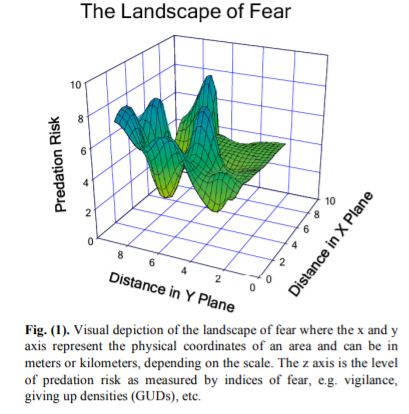
Laundre et al. (2010) present a visual representation of the landscape of fear (Fig. 1, reproduced below), where as an animal moves through space (represented as distance in meters or kilometers, for example), they also move through varying levels of predation risk. Environmental gradients (temperature, for example) tend to be much more stable across space in terrestrial ecosystems such as in the Yellowstone example from the paper. I wonder whether the same concept and visual depiction of a landscape of fear could be translated as risk across various environmental gradients, rather than geographic distances? In this proposed illustration, a landscape of fear would vary based on gradients of environmental conditions rather than geographic space. Such a shift in spatial reference —from geographic to environmental space—might make the model more applicable in the dynamic ocean ecosystems that we study.
What about cases when the predators we study become prey? One example we discussed was gray whales migrating from breeding lagoons in Mexico to feeding grounds in the Bering Sea. Mother-calf pairs hug the coastline tightly, by no means taking the most direct route between locations and adding considerable travel distance to their migration. The leading hypothesis is that mother gray whales take the coastal route to minimize the risk that their calves will fall prey to killer whale attacks. Are there other cases where the predators we study operate in a seascape of fear that we do not yet understand? Likely so, and the predators’ own seascape of fear may account for cases when we cannot explain predator distribution simply by their prey and their environment. To take this a step further, it might be beneficial not only to think of predation risk as only the potential to be eaten, but expand our definition to include human disturbance. While humans may not directly prey on marine predators, the disturbance from human activity in the ocean likely creates a layer of fear which animals must navigate, even in the absence of actual predation.
Our lively lab meeting discussion prompted me to look into
how the landscape of fear model has been applied to the highly dynamic and
intricate marine environment. In a study examining predator-prey dynamics of
three species of marine mammals—bottlenose dolphins, harbor seals, and
dugongs—Wirsing et al. (2007) found that in all three cases, the study species
spent less time in more desirable prey patches or decreased riskier behavior in
the presence of predators. Most studies in marine ecology are observational, as
we rarely have the opportunity to manipulate our study system for experimental
design and hypothesis testing. However, a study of coral reefs in the Florida
Keys conducted by Catano et al. (2015) used fabricated predators—decoys of
black grouper, a predatory fish—to investigate the influence of fear of
predation on the reef system. What they found was that herbivorous fish
consumed significantly less and fed at a much faster rate in the presence of this
decoy predator. The grouper, even in decoy form, created a “reefscape of fear”,
altering patterns in herbivory with potential ramifications for the entire ecosystem.
My takeaway from our discussion and my musings in this
week’s blog post is that predator and prey distribution and behavior is highly
interconnected. While predators distribute themselves to maximize their ability
to find a meal, their prey respond accordingly by balancing finding a meal of
their own with minimizing the risk that they will be eaten. Ecology is the
study of an ecosystem, which means the questions we ask are complicated and
hierarchical, and must be considered from multiple angles, accounting for
biological, environmental, and behavioral elements to name a few. These
challenges of studying ecosystems are simultaneously what make ecology
fascinating, and exciting.
References:
Laundré, J. W., Hernández, L., & Ripple, W. J. (2010).
The landscape of fear: ecological implications of being afraid. Open
Ecology Journal, 3, 1-7.
Catano, L. B., Rojas, M. C., Malossi, R. J., Peters, J. R.,
Heithaus, M. R., Fourqurean, J. W., & Burkepile, D. E. (2016). Reefscapes
of fear: predation risk and reef hetero‐geneity interact to shape herbivore
foraging behaviour. Journal of Animal Ecology, 85(1),
146-156.
Wirsing, A. J., Heithaus, M. R., Frid, A., & Dill, L. M.
(2008). Seascapes of fear: evaluating sublethal predator effects experienced
and generated by marine mammals. Marine Mammal Science, 24(1),
1-15.
By Lisa Hildebrand, MSc student, OSU Department of Fisheries and Wildlife, Geospatial Ecology of Marine Megafauna Lab
It seems unfathomable to me that one year and two months ago I had never used a theodolite before, never been in an ocean kayak before, never identified zooplankton before, never seen a Time-Depth-Recorder (TDR) before. Now, one year later, it seems like all of those tools, techniques and things are just a couple of old friends with which I am being reunited with again. My second field season as the project team lead of the gray whale foraging ecology project in Port Orford (PO) is slowly getting underway and so many of the lessons I learned from my first field season last year have already helped me tremendously this year. I know how to interpret weather forecasts and determine whether it will be a kayak-appropriate day. I know how to figure out the quirks of Pythagoras, the program we use to interface with our theodolite which helps us track whales from our cliff site. I know how to keep track of a budget and feed a team of hungry researchers after a long day of work. Knowing all of these things ahead of this year’s field season have made me feel a little more prepared and at ease with the training of my team and the work to be done. Nevertheless, there are always new curveballs to be thrown my way and while they can often be frustrating, I enjoy the challenges that being a team leader has to offer as it allows me to continue to grow as a field research scientist.
Figure 1. Crew Cinco tracks a whale in Tichenor Cove. Source: L Hildebrand.
2019 marks the fifth year that this project has been taking place in PO. Back in the summer of 2015, former GEMM Lab Master’s student Florence Sullivan started this project together with Leigh. That year the research focused more on investigating vessel disturbance to gray whales by comparing sites of heavy (Boiler Bay) to low boat traffic (Port Orford). The effort found that there were significant differences in gray whale activity budgets between the heavy and low boat traffic conditions (Sullivan & Torres 2018). The following year, the focus of the research switched to being more on the foraging ecology side of things and the project was based solely out of Port Orford, as it continues to be to this day. Being in our fifth year means that we are starting to build a humbly-sized database of sightings across multiple years allowing me to investigate potential individual specialization of the whales that we document. Similarly, multiple years of prey sampling is starting to reveal temporal and spatial trends of prey community assemblages.
Figure 2. Buttons (pictured above) is one of the stars of the Port Orford gray whale foraging ecology project as he has been seen every year since 2016. Crew Cinco has already seen him three times since the start of August. Source: L Hildebrand.
It has become a tradition to come up with a name for the field team that spends 6 weeks at the Oregon State University (OSU) Port Orford Field Station to collect the data for the project. It started with Team Ro“buff”stus in 2015, which I believe carried through until 2017. This is understandable since it’s such a clever name. It’s a play on the species name for gray whales, robustus, but the word “Buff” has been substituted in the center. Buffs are pieces of cloth sewn into a cylindrical shape, often with fun patterns or colors, that can be used as face masks, headbands, and scarves, which come in very handy when your face is exposed to the elements. Doing this project, we can be confronted by wind, sun, fog and sea water all in one day, so Buffs have definitely served the team members very well over the years. Last year, as the project’s torch was passed from Florence to myself, I felt a new team name was apt, and so last year’s team decided our name would be Team Whale Storm. I believe it was because we said we would take the whale world by storm with our insanely good theodolite tracking and kayak sampling skills. With a new year and new team upon us, a new team name was in order. As the title of this blog post indicates, this year the team is called Crew Cinco. The reason behind this name is that we are the fifth team to carry out this field work. Since the gray whales breed in the lagoons of Baja California, Mexico, I like to think that their native language is Spanish. Hence, we have decided that instead of being Crew Five, we are Crew Cinco, as cinco is the Spanish word for five (besides, alliteration makes for a much better team name).
Now that you are up to speed on the history of the PO gray whale project, let me tell you a little about who is part of Crew Cinco and what we have been up to already.
This year’s Marine Studies Initiative OSU undergraduate intern is Mia Arvizu. Mia has just finished her sophomore year at OSU and majors in Environmental Science. Besides being my co-captain this year in the field, Mia is also undertaking an independent research project which focuses on the relationship between sea urchin abundance, kelp health and gray whale foraging. She will tell you all about this project in a few weeks when she takes over the GEMM lab blog. Aside from her interest in ecology and the way science can be used to help local communities in a changing environment, Mia is a dancer, having performed in several dances in OSU’s annual luau this year, and she is currently teaching herself Spanish and Hawaiian.
Both of our high school interns this year are from Astoria. Anthony Howe has just graduated from Astoria High School and will be starting at Clatsop Community College in the fall. His plan is to transfer to OSU and to pursue his interest in marine biology. Anthony, like myself, was born in Germany and lived there until he was six, which means that he is able to speak fluent German. He also introduced the team to the wonders of the Instant Pot, which has made cooking for a team of four hungry scientists much simpler.
Donovan Burns is our other high school intern. He will be going into his junior year in the fall. Donovan never ceases to amaze us with the seemingly endless amounts of general knowledge he has, often sharing facts about Astoria’s history to Asimov’s Laws of Robotics to pickling vegetables, specifically carrots, with us during dinner or while scanning for whales on the cliff site. He also named the first whale we saw here this season – Speckles.
Figure 3. Crew Cinco, from left to right: Anthony Howe, Donovan Burns, Lisa Hildebrand and Mia Arvizu. Source: L Torres.
Crew Cinco has already been in PO for two weeks now. After having a full team meeting with Leigh in Newport and a GEMM lab summer pizza party, we headed south to begin our 6-week field season. It’s hard to believe that the two training weeks are already over. The team worked hard to figure out the subtleties of the theodolite, observe different gray whales and start to understand their dive and foraging patterns, undertake a kayak paddle & safety course, as well as CPR and First Aid training, learn about data processing and management, and how to use a variety of gizmos to aid us in data collection. But it hasn’t all been work. We enjoyed a day in the Californian Redwoods on one of our day’s off and picked blueberries at the Twin Creek Ranch, stocking our freezer with several bags of juicy berries. We have played ‘Sorry!’ perhaps one too many times already (we are in desperate need of some more boardgames if anyone wants to send some our way to the field station!), and enjoyed many walks and runs on beautiful Battle Rock Beach.
Crew Cinco in awe of the Redwoods
Crew Cinco’s blueberry harvest
Crew Cinco after their kayak paddle & safety course South Coast Tours
The next four weeks will not be easy – very early mornings, lots of paddling and squinting into the sun, followed by several hours in the lab processing samples and backing up data. But the next four weeks will also be extremely rewarding – learning lots of new skills that will be valuable beyond this 6-week period, revealing ecological trends and relationships, and ultimately (the true reason for why Mia, Anthony, Donovan and myself are more than happy to put in 6 weeks-worth of hard work), the chance to see whales every day up close and personal. Follow Crew Cinco’s journey over the next few weeks as my interns will be posting to the blog for the next three weeks!
References
Sullivan, F.A., & Torres L.G. Assessment of vessel disturbance to gray whales to inform sustainable ecotourism. Journal of Wildlife Management, 2018. 82: 896-905.
By Dominique Kone, Masters Student in Marine Resource Management
By now, I’m sure you’re aware of recent interests to reintroduce sea otters to Oregon. To inform this effort, my research focuses on predicting suitable sea otter habitat and investigating the potential ecological effects if sea otters are reintroduced in the future. This information will help managers gain a better understanding of the potential for sea otters to reestablish in Oregon, as well as how Oregon’s ecosystems may change via top-down processes. These analyses will address some sources of uncertainties of this effort, but there are still many more questions researchers could address to further guide this process. Here, I note some lingering questions I’ve come across in the course of conducting my research. This is not a complete list of all questions that could or should be investigated, but they represent some of the most interesting questions I have and others have in Oregon.
Credit: Todd Mcleish
The questions, and our associated knowledge on each of these topics:
Is there enough available prey to support a robust sea otter population in Oregon?
Sea otters require approximately 30% of their own body weight in food every day (Costa 1978, Reidman & Estes 1990). With a large appetite, they not only need to spend most of their time foraging, but require a steady supply of prey to survive. For predators, we assume the presence of suitable habitat is a reliable proxy for prey availability (Redfern et al. 2006). Whereby, quality habitat should supply enough prey to sustain predators at higher trophic levels.
In making these habitat predictions for sea otters, we must also recognize the potential limitations of this “habitat equals prey” paradigm, in that there may be parcels of habitat where prey is unavailable or inaccessible. In Oregon, there could be unknown processes unique to our nearshore ecosystems that would support less prey for sea otters. This possibility highlights the importance of not only understanding how much suitable habitat is available for foraging sea otters, but also how much prey is available in these habitats to sustain a viable otter population in the future. Supplementing these habitat predictions with fishery-independent prey surveys is one way to address this question.
Credit: Suzi Eszterhas via Smithsonian Magazine
How will Oregon’s oceanographic seasonality alter or impact habitat suitability?
Sea otters along the California coast exist in an environment with persistent Giant kelp beds, moderate to low wave intensity, and year-round upwelling regimes. These environmental variables and habitat factors create productive ecosystems that provide quality sea otter habitat and a steady supply of prey; thus, supporting high densities of sea otters. This environment contrasts with the Oregon coast, which is characterized by seasonal changes in bull kelp and wave intensity. Summer months have dense kelp beds, calm surf, and strong upwellings. While winter months have little to no kelp, weak upwellings, and intense wave climates. These seasonal variations raise the question as to how these temporal fluctuations in available habitat could impact the number of sea otters able to survive in Oregon.
In Washington – an environment like Oregon – sea otters exhibit seasonal distribution patterns in response to intensifying wave climates. During calm summer months, sea otters primarily forage along the outer coast, but move into more protected areas, such as the Strait of Juan de Fuca, during winter months (Laidre et al. 2009). If sea otters were reintroduced to Oregon, we may very well observe similar seasonal movement patterns (e.g. dispersal into estuaries), but the degree to which this seasonal redistribution and reduction in foraging habitat could impact sea otter reestablishment and recovery is currently unknown.
Credit: Oregon Coast Aquarium
In the event of a reintroduction, do northern or southern sea otters have a greater capacity to adapt to Oregon environments?
In the early 1970’s, Oregon’s first sea otter translocation effort failed (Jameson et al. 1982). Since then, hypotheses on the potential ecological differences between northern and southern sea otters have been proposed as potential factors of the failed effort, potentially due to different abilities to exploit specific prey species. Studies have demonstrated that northern and southern sea otters have slight morphological differences – northern otters having larger skulls and teeth than southern otters (Wilson et al. 1991). This finding has created the hypothesis that the northern otter’s larger skull and teeth allow it to consume prey with denser exoskeletons, and thereby can exploit a greater diversity of prey species. However, there appears to be a lack of evidence to suggest larger skulls and teeth translate to greater bite force. Based on morphology alone, either sub-species could be just as successful in exploiting different prey species.
A different direction to address questions around adaptability is to look at similarities in habitat and oceanographic characteristics. Sea otters exist along a gradient of habitat types (e.g. kelp forests, estuaries, soft-sediment environments) and oceanographic conditions (e.g. warm-temperature to cooler sub-Arctic waters) (Laidre et al. 2009, Lafferty et al. 2014). Yet, we currently don’t know how well or quickly otters can adapt when they expand into new habitats that differ from ones they are familiar with. Sea otters must be efficient foragers and need to acquire skills that allow them to effectively hunt specific prey species (Estes et al. 2003). Hypothetically, if we take sea otters from rocky environments where they’ve developed foraging skills to hunt sea urchins and abalones, and place them in a soft-sediment environment, how quickly would they develop new foraging skills to exploit soft-sediment prey species? Would they adapt quickly enough to meet their daily prey requirements?
Credit: Eric Risberg/Associated Press via The Columbian
In Oregon, specifically, how might climate change impact sea otters, and how might sea otters mediate climate impacts?
Climate change has been shown to directly impact many species via changes in temperature (Chen et al. 2011). Some species have specific thermal tolerances, in which they can only survive within a specified temperature range (i.e. maximum and minimum). Once the temperature moves out of that range, the species can either move with those shifting water masses, behaviorally adapt or perish (Sunday et al. 2012). It’s unclear if and how changing temperatures will impact sea otters, directly. However, sea otters could still be indirectly affected via impacts to their prey. If prey species in sea otter habitat decline due to changing temperatures, this would reduce available food for otters. Ocean acidification (OA) is another climate-induced process that could indirectly impact sea otters. By creating chemical conditions that make it difficult for species to form shells, OA could decrease the availability of some prey species, as well (Gaylord et al. 2011).
Interestingly, these pathways between sea otters and climate change become more complex when we consider the potentially mediating effects from sea otters. Aquatic plants – such as kelp and seagrass – can reduce the impacts of climate change by absorbing and taking carbon out of the water column (Krause-Jensen & Duarte 2016). This carbon sequestration can then decrease acidic conditions from OA and mediate the negative impacts to shell-forming species. When sea otters catalyze a tropic cascade, in which herbivores are reduced and aquatic plants are restored, they could increase rates of carbon sequestration. While sea otters could be an effective tool against climate impacts, it’s not clear how this predator and catalyst will balance each other out. We first need to investigate the potential magnitude – both temporal and spatial – of these two processes to make any predictions about how sea otters and climate change might interact here in Oregon.
Credit: National Wildlife Federation
In Summary
There are several questions I’ve noted here that warrant further investigation and could be a focus for future research as this potential sea otter reintroduction effort progresses. These are by no means every question that should be addressed, but they do represent topics or themes I have come across several times in my own research or in conversations with other researchers and managers. I think it’s also important to recognize that these questions predominantly relate to the natural sciences and reflect my interest as an ecologist. The number of relevant questions that would inform this effort could grow infinitely large if we expand our disciplines to the social sciences, economics, genetics, so on and so forth. Lastly, these questions highlight the important point that there is still a lot we currently don’t know about (1) the ecology and natural behavior of sea otters, and (2) what a future with sea otters in Oregon might look like. As with any new idea, there will always be more questions than concrete answers, but we – here in the GEMM Lab – are working hard to address the most crucial ones first and provide reliable answers and information wherever we can.
References:
Chen, I., Hill, J. K., Ohlemuller, R., Roy, D. B., and C. D. Thomas. 2011. Rapid range shifts of species associated with high levels of climate warming. Science. 333: 1024-1026.
Costa, D. P. 1978. The ecological energetics, water, and electrolyte balance of the California sea otter (Enhydra lutris). Ph.D. dissertation, University of California, Santa Cruz.
Estes, J. A., Riedman, M. L., Staedler, M. M., Tinker, M. T., and B. E. Lyon. 2003. Individual variation in prey selection by sea otters: patterns, causes and implications. Journal of Animal Ecology. 72: 144-155.
Gaylord et al. 2011. Functional impacts of ocean acidification in an ecologically critical foundation species. Journal of Experimental Biology. 214: 2586-2594.
Jameson, R. J., Kenyon, K. W., Johnson, A. M., and H. M. Wight. 1982. History and status of translocated sea otter populations in North America. Wildlife Society Bulletin. 10(2): 100-107.
Krause-Jensen, D., and C. M. Duarte. 2016. Substantial role of macroalgae in marine carbon sequestration. Nature Geoscience. 9: 737-742.
Lafferty, K. D., and M. T. Tinker. 2014. Sea otters are recolonizing southern California in fits and starts. Ecosphere.5(5).
Laidre, K. L., Jameson, R. J., Gurarie, E., Jeffries, S. J., and H. Allen. 2009. Spatial habitat use patterns of sea otters in coastal Washington. Journal of Marine Mammalogy. 90(4): 906-917.
Redfern et al. 2006. Techniques for cetacean-habitat modeling. Marine Ecology Progress Series. 310: 271-295.
Reidman, M. L. and J. A. Estes. 1990. The sea otter (Enhydra lutris): behavior, ecology, and natural history. United States Department of the Interior, Fish and Wildlife Service, Biological Report. 90: 1-126.
Sunday, J. M., Bates, A. E., and N. K. Dulvy. 2012. Thermal tolerance and the global redistribution of animals. Nature: Climate Change. 2: 686-690.
Wilson, D. E., Bogan, M. A., Brownell, R. L., Burdin, A. M., and M. K. Maminov. 1991. Geographic variation in sea otters, Ehydra lutris. Journal of Mammalogy. 72(1): 22-36.
By Christina Garvey, University of Maryland, GEMM Lab REU Intern
It is July 8th and it is my 4th week here in Hatfield as an REU intern for Dr. Leigh Torres. My name is Christina Garvey and this summer I am studying the spatial ecology of blue whales in the South Taranaki Bight, New Zealand. Coming from the east coast, Oregon has given me an experience of a lifetime – the rugged shorelines continue to take my breath away and watching sea lions in Yaquina Bay never gets old. However, working on my first research project has by far been the greatest opportunity and I have learned so much in so little time. When Dr. Torres asked me to contribute to this blog I was unsure of how I would write about my work thus far but I am excited to have the opportunity to share the knowledge I have gained with whoever reads this blog post.
The research project that I will be conducting this summer will use remotely sensed environmental data (information collected from satellites) to predict blue whale distribution in the South Taranaki Bight (STB), New Zealand. Those that have read previous blogs about this research may remember that the STB study area is created by a large indentation or “bight” on the southern end of the Northern Island. Based on multiple lines of evidence, Dr. Leigh Torres hypothesized the presence of an unrecognized blue whale foraging ground in the STB (Torres 2013). Dr. Torres and her team have since proved that blue whales frequent this region year-round; however, the STB is also very industrial making this space-use overlap a conservation concern (Barlow et al. 2018). The increasing presence of marine industrial activity in the STB is expected to put more pressure on blue whales in this region, whom are already vulnerable from the effects of past commercial whaling (Barlow et al. 2018) If you want to read more about blue whales in the STB check out previous blog posts that talk all about it!
Figure 1. A blue whale surfaces in front of a floating production storage and offloading vessel servicing the oil rigs in the South Taranaki Bight. Photo by D. Barlow.
Figure 2. South Taranaki Bight, New Zealand, our study site outlined by the red box. Kahurangi Point (black star) is the site of wind-driven upwelling system.
The possibility of the STB as an important foraging ground for a resident population of blue whales poses management concerns as New Zealand will have to balance industrial growth with the protection and conservation of a critically endangered species. As a result of strong public support, there are political plans to implement a marine protected area (MPA) in the STB for the blue whales. The purpose of our research is to provide scientific knowledge and recommendations that will assist the New Zealand government in the creation of an effective MPA.
In order to create an MPA that would help conserve the blue whale population in the STB, we need to gather a deeper understanding of the relationship between blue whales and this marine environment. One way to gain knowledge of the oceanographic and ecological processes of the ocean is through remote sensing by satellites, which provides accessible and easy to use environmental data. In our study we propose remote sensing as a tool that can be used by managers for the design of MPAs (through spatial and temporal boundaries). Satellite imagery can provide information on sea surface temperature (SST), SST anomaly, as well as net primary productivity (NPP) – which are all measurements that can help describe oceanographic upwelling, a phenomena that is believed to be correlated to the presence of blue whales in the STB region.
Figure 3. The stars of the show: blue whales. A photograph captured from the small boat of one animal fluking up to dive down as another whale surfaces close by. (Photo credit: L. Torres)
Past studies in the STB showed evidence of a large upwelling event that occurs off the coast of Kahurangi Point (Fig. 2), on the northwest tip of the South Island (Shirtcliffe et al. 1990). In order to study the relationship of this upwelling to the distribution of blue whales, I plan to extract remotely sensed data (SST, SST anomaly, & NPP) off the coast of Kahurangi and compare it to data gathered from a centrally located site within the STB, which is close to oil rigs and so is of management interest. I will first study how decreases in sea surface temperature at the site of upwelling (Kahurangi) are related to changes in sea surface temperature at this central site in the STB, while accounting for any time differences between each occurrence. I expect that this relationship will be influenced by the wind patterns, and that there will be changes based on the season. I also predict that drops in temperature will be strongly related to increases in primary productivity, since upwelling brings nutrients important for photosynthesis up to the surface. These dips in SST are also expected to be correlated to blue whale occurrence within the bight, since blue whale prey (krill) eat the phytoplankton produced by the productivity.
Figure 4. A blue whale lunges on an aggregation of krill. UAS piloted by Todd Chandler.
To test the relationships I determine between remotely sensed data at different locations in the STB, I plan to use blue whale observations from marine mammal observers during a seismic survey conducted in 2013, as well as sightings recorded from the 2014, 2016, and 2017 field studies led by Dr. Leigh Torres. By studying the statistical relationships between all of these variables I hope to prove that remote sensing can be used as a tool to study and understand blue whale distribution.
I am very excited about this research, especially because the end goal of creating an MPA really gives me purpose. I feel very lucky to be part of a project that could make a positive impact on the world, if only in just a little corner of New Zealand. In the mean time I’ll be here in Hatfield doing the best I can to help make that happen.
References:
Barlow DR, Torres LG, Hodge KB, Steel D, Baker CS, Chandler TE, Bott N, Constantine R, Double MC, Gill P, Glasgow D, Hamner RM, Lilley C, Ogle M, Olson PA, Peters C, Stockin KA, Tessaglia-hymes CT, Klinck H (2018) Documentation of a New Zealand blue whale population based on multiple lines of evidence. Endanger Species Res 36:27–40.
Shirtcliffe TGL, Moore MI, Cole AG, Viner AB, Baldwin R, Chapman B (1990) Dynamics of the Cape Farewell upwelling plume, New Zealand. New Zeal J Mar Freshw Res 24:555–568.
Torres LG (2013) Evidence for an unrecognised blue whale foraging ground in New Zealand. New Zeal J Mar Freshw Res 47:235–248.
Just like that, I have wrapped up year 1 of my PhD in Wildlife Science. For my PhD, I am investigating the ecology and distribution of blue whales in New Zealand across multiple spatial and temporal scales. In a region where blue whales overlap with industrial activity, there is considerable interest from managers to be able to reliably forecast when and where blue whales are most likely to be in the area. In a series of five chapters and utilizing multiple different data sources (dedicated boat surveys, oceanographic data, acoustic recordings, remotely sensed environmental data, opportunistic blue whale sightings information), I will attempt to describe, quantify, and predict where blue whales are found in relation to their environment. Each chapter will evaluate the distribution of blue whales relative to the environment at different scales in space (ranging from 4 km to 25 km resolution) and time (ranging from daily to seasonal resolution). One overarching method I am using throughout my PhD is species distribution modeling. Having just completed my research review with my doctoral committee last week, I’ll share this aspect of my research proposal that I’ve particularly enjoyed reading, writing, and thinking about.
A pair of blue whales surfacing in the South Taranaki Bight region of New Zealand. Drone piloted by Todd Chandler during the 2017 field season.
Species distribution models (SDMs), which are sometimes referred to as habitat models or ecological niche models, are mathematical algorithms that combine observations of a species with environmental conditions at their observed locations, to gain ecological insight and predict spatial distributions of the species (Elith and Leathwick, 2009; Redfern et al., 2006). Any model is just one description of what is occurring in the natural world. Just as there are many ways to describe something with words and many languages to do so, there are many options for modeling frameworks and approaches, with stark and nuanced differences. My labmate and friend Solene Derville has equated the number of choices one has for SDMs to the cracker section in an American grocery store. When navigating all of these choices and considerations, it is important to remember that no model will ever be completely correct—it is our best attempt at describing a complex natural system—and as an analyst we need to do the best that we can with the data available to address the ecological questions at hand. As it turns out, the dividing line between quantitative analysis and philosophy is thin at times. What may seem at first like a purely objective, statistical endeavor requires careful consideration and fundamental decision-making on the part of the analyst.
Ecosystems are multifaceted, complex, and hierarchical. They are comprised of multiple physical and biological components, which operate at multiple scales across space and time. As Dr. Simon Levin stated in at 1989 MacArthur Award lecture on the topic of scale in ecology:
“A good model does not attempt to reproduce every detail of the biological system; the system itself suffices for that purpose as the most detailed model of itself. Rather, the objective of a model should be to ask how much detail can be ignored without producing results that contradict specific sets of observations, on particular scales of interest” (Levin, 1992).
The question of scale is central to ecology. As many biology students learn in their first introductory classes, parsimony is “The principle that the most acceptable explanation of an occurrence, phenomenon, or event is the simplest, involving the fewest entities, assumptions, or changes” (Oxford Dictionary). In other words, the best explanation is the simplest one. One challenge in ecological modeling, including SDMs, is to select spatial and temporal scales as coarse as possible for the most parsimonious—the most straightforward—model, while still being fine enough to capture relevant patterns. Another critical consideration is the scale of the question you are interested in answering. The scale of the analysis must match the scale at which you want to make inferences about the ecology of a species.
Similarly, the issue of complexity is central to distribution modeling. Overly simple models may not be able to adequately describe the relationship between species occurrence and the environment. In contrast, highly complex models may have very high explanatory power, but risk ascribing an ecological pattern to noise in the data (Merow et al., 2014), in other words, finding patterns that aren’t real. Furthermore, highly complex models tend to have poorer predictive capacity than simpler models (Merow et al., 2014). There is a trade-off between descriptive and predictive power in SDMs (Derville et al., 2018). Therefore, a key component in the SDM process is establishing the end goal of the model with respect to the region of interest, scale, explanatory power, predictive capacity, and in many cases management need.
Finally, any model is ultimately limited by the data available and the scale at which it was collected (Elith and Leathwick, 2009; Guillera-Arroita et al., 2015; Redfern et al., 2006). Prior knowledge of what environmental features are important to the species of interest is often limited at the time of the data collection effort, and data collection is constrained by when it is logistically feasible to sample. For example, we collect detailed oceanographic data during the summer months when it is practical to get out on the water, satellite imagery of sea surface temperature might be unavailable during times of cloud cover, and people are more likely to report blue whale sightings in areas where there is more human activity. Therefore, useful SDMs that address both ecological and management needs typically balance the scale of analysis and model complexity with the limitations of the data.
Managers and politicians within the New Zealand government are interested in a tool to predict when and where blue whales are most likely to be, based on sound ecological analysis. This is one of the end-goals of my PhD, but in the meantime, I am grappling with the appropriate scales of analysis, and attempting to balance questions of model complexity, explanatory power, and predictive capacity. There is no single, correct answer, and so my process is in part quantitative analysis, part philosophy, and all with the goal of increased ecological understanding and conservation of a species.
A blue whale breaks the surface. As I grapple with questions of model complexity and scale of analysis, I sometimes need a reminder that behind each data point is a blue whale, and what a privilege it is to study them. Photo by Leigh Torres.
References:
Derville, S., Torres, L. G., Iovan, C., and Garrigue, C. (2018). Finding the right fit: Comparative cetacean distribution models using multiple data sources and statistical approaches. Divers. Distrib. 24, 1657–1673. doi:10.1111/ddi.12782.
Elith, J., and Leathwick, J. R. (2009). Species Distribution Models: Ecological Explanation and Prediction Across Space and Time. Annu. Rev. Ecol. Evol. Syst. 40, 677–697. doi:10.1146/annurev.ecolsys.110308.120159.
Guillera-Arroita, G., Lahoz-Monfort, J. J., Elith, J., Gordon, A., Kujala, H., Lentini, P. E., et al. (2015). Is my species distribution model fit for purpose? Matching data and models to applications. Glob. Ecol. Biogeogr. 24, 276–292. doi:10.1111/geb.12268.
Levin, S. A. (1992). The problem of pattern and scale. Ecology 73, 1943–1967.
Merow, C., Smith, M. J., Edwards, T. C., Guisan, A., Mcmahon, S. M., Normand, S., et al. (2014). What do we gain from simplicity versus complexity in species distribution models? Ecography (Cop.). 37, 1267–1281. doi:10.1111/ecog.00845.
Redfern, J. V., Ferguson, M. C., Becker, E. A., Hyrenbach, K. D., Good, C., Barlow, J., et al. (2006). Techniques for cetacean-habitat modeling. Mar. Ecol. Prog. Ser. 310, 271–295. doi:10.3354/meps310271.
By: Alexa Kownacki, Ph.D. Student, OSU Department of Fisheries and Wildlife, Geospatial Ecology of Marine Megafauna Lab
Data analysis is often about parsing down data into manageable subsets. My project, which spans 34 years and six study sites along the California coast, requires significant data wrangling before full analysis. As part of a data analysis trial, I first refined my dataset to only the San Diego survey location. I chose this dataset for its standardization and large sample size; the bulk of my sightings, over 4,000 of the 6,136, are from the San Diego survey site where the transect methods were highly standardized. In the next step, I selected explanatory variable datasets that covered the sighting data at similar spatial and temporal resolutions. This small endeavor in analyzing my data was the first big leap into understanding what questions are feasible in terms of variable selection and analysis methods. I developed four major hypotheses for this San Diego site.
The study species: common bottlenose dolphin (Tursiops truncatus) seen along the California coastline in 2015. Image source: Alexa Kownacki.
Hypotheses:
H1: I predict that bottlenose dolphin sightings along the San Diego transect throughout the years 1981-2015 exhibit clustered distribution patterns as a result of the patchy distributions of both the species’ preferred habitats, as well as the social nature of bottlenose dolphins.
H2: I predict there would be higher densities of bottlenose dolphin at higher latitudes spanning 1981-2015 due to prey distributions shifting northward and less human activities in the northerly sections of the transect.
H3: I predict that during warm (positive) El Niño Southern Oscillation (ENSO) months, the dolphin sightings in San Diego would be distributed more northerly, predominantly with prey aggregations historically shifting northward into cooler waters, due to (secondarily) increasing sea surface temperatures.
H4: I predict that along the San Diego coastline, bottlenose dolphin sightings are clustered within two kilometers of the six major lagoons, with no specific preference for any lagoon, because the murky, nutrient-rich waters in the estuarine environments are ideal for prey protection and known for their higher densities of schooling fishes.
Data Description:
The common bottlenose dolphin (Tursiops truncatus) sighting data spans 1981-2015 with a few gap years. Sightings cover all months, but not in all years sampled. The same transect in San Diego was surveyed in a small, rigid-hulled inflatable boat with approximately a two-kilometer observation area (one kilometer surveyed 90 degrees to starboard and port of the bow).
I wanted to see if there were changes in dolphin distribution by latitude and, if so, whether those changes had a relationship to ENSO cycles and/or distances to lagoons. For ENSO data, I used the NOAA database that provides positive, neutral, and negative indices (1, 0, and -1, respectively) by each month of each year. I matched these ENSO data to my month-date information of dolphin sighting data. Distance from each lagoon was calculated for each sighting.
Figure 1. Map representing the San Diego transect, represented with a light blue line inside of a one-kilometer buffered “sighting zone” in pale yellow. The dark pink shapes are dolphin sightings from 1981-2015, although some are stacked on each other and cannot be differentiated. The lagoons, ranging in size, are color-coded. The transect line runs from the breakwaters of Mission Bay, CA to Oceanside Harbor, CA.
Results:
H1:True, dolphins are clustered and do not have a uniform distribution across this area. Spatial analysis indicated a less than a 1% likelihood that this clustered pattern could be the result of random chance (Fig. 1, z-score = -127.16, p-value < 0.0001). It is well-known that schooling fishes have a patchy distribution, which could influence the clustered distribution of their dolphin predators. In addition, bottlenose dolphins are highly social and although pods change in composition of individuals, the dolphins do usually transit, feed, and socialize in small groups.
Figure 2. Summary from the Average Nearest Neighbor calculation in ArcMap 10.6 displaying that bottlenose dolphin sightings in San Diego are highly clustered. When the z-score, which corresponds to different colors on the graphic above, is strongly negative (< -2.58), in this case dark blue, it indicates clustering. Because the p-value is very small, in this case, much less than 0.01, these results of clustering are strongly significant.
H2:False, dolphins do not occur at higher densities in the higher latitudes of the San Diego study site. The sightings are more clumped towards the lower latitudes overall (p < 2e-16), possibly due to habitat preference. The sightings are closer to beaches with higher human densities and human-related activities near Mission Bay, CA. It should be noted, that just north of the San Diego transect is the Camp Pendleton Marine Base, which conducts frequent military exercises and could deter animals.
Figure 3. Histogram comparing the latitudes with the frequency of dolphin sightings in San Diego, CA. The x-axis represents the latitudinal difference from the most northern part of the transect to each dolphin sighting. Therefore, a small difference would translate to a sighting being in the northern transect areas whereas large differences would translate to sightings being more southerly. This could be read from left to right as most northern to most southern. The y-axis represents the frequency of which those differences are seen, that is, the number of sightings with that amount of latitudinal difference, or essentially location on the transect line. Therefore, you can see there is a peak in the number of sightings towards the southern part of the transect line.
H3: False, during warm (positive) El Niño Southern Oscillation (ENSO) months, the dolphin sightings in San Diego were more southerly. In colder (negative) ENSO months, the dolphins were more northerly. The differences between sighting latitude and ENSO index was significant (p<0.005). Post-hoc analysis indicates that the north-south distribution of dolphin sightings was different during each ENSO state.
Figure 4. Boxplot visualizing distributions of dolphin sightings latitudinal differences and ENSO index, with -1,0, and 1 representing cold, neutral, and warm years, respectively.
H4:True, dolphins are clustered around particular lagoons. Figure 5 illustrates how dolphin sightings nearest to Lagoon 6 (the San Dieguito Lagoon) are always within 0.03 decimal degrees. Because of how these data are formatted, decimal degrees is the easiest way to measure change in distance (in this case, the difference in latitude). In comparison, dolphins at Lagoon 5 (Los Penasquitos Lagoon) are distributed across distances, with the most sightings further from the lagoon.
Figure 5. Bar plot displaying the different distances from dolphin sighting location to the nearest lagoon in San Diego in decimal degrees. Note: Lagoon 4 is south of the study site and therefore was never the nearest lagoon.
I found a significant difference between distance to nearest lagoon in different ENSO index categories (p < 2.55e-9): there is a significant difference in distance to nearest lagoon between neutral and negative values and positive and neutral years. Therefore, I hypothesize that in neutral ENSO months compared to positive and negative ENSO months, prey distributions are changing. This is one possible hypothesis for the significant difference in lagoon preference based on the monthly ENSO index. Using a violin plot (Fig. 6), it appears that Lagoon 5, Los Penasquitos Lagoon, has the widest variation of sighting distances in all ENSO index conditions. In neutral years, Lagoon 0, the Buena Vista Lagoon has multiple sightings, when in positive and negative years it had either no sightings or a single sighting. The Buena Vista Lagoon is the most northerly lagoon, which may indicate that in neutral ENSO months, dolphin pods are more northerly in their distribution.
Figure 6. Violin plot illustrating the distance from lagoons of dolphin sightings under different ENSO conditions. There are three major groups based on ENSO index: “-1” representing cold years, “0” representing neutral years, and “1” representing warm years. On the x-axis are lagoon IDs and on the y-axis is the distance to the nearest lagoon in decimal degrees. The wider the shapes, the more sightings, therefore Lagoon 6 has many sightings within a very small distance compared to Lagoon 5 where sightings are widely dispersed at greater distances.
Bottlenose dolphins foraging in a small group along the California coast in 2015. Image source: Alexa Kownacki.
Takeaways to science and management:
Bottlenose dolphins have a clustered distribution which seems to be related to ENSO monthly indices, and likely, their social structures. From these data, neutral ENSO months appear to have something different happening compared to positive and negative months, that is impacting the sighting distributions of bottlenose dolphins off the San Diego coastline. More research needs to be conducted to determine what is different about neutral months and how this may impact this dolphin population. On a finer scale, the six lagoons in San Diego appear to have a spatial relationship with dolphin sightings. These lagoons may provide critical habitat for bottlenose dolphins and/or for their preferred prey either by protecting the animals or by providing nutrients. Different lagoons may have different spans of impact, that is, some lagoons may have wider outflows that create larger nutrient plumes.
Other than the Marine Mammal Protection Act and small protected zones, there are no safeguards in place for these dolphins, whose population hovers around 500 individuals. Therefore, specific coastal areas surrounding lagoons that are more vulnerable to habitat loss, habitat degradation, and/or are more frequented by dolphins, may want greater protection added at a local, state, or federal level. For example, the Batiquitos and San Dieguito Lagoons already contain some Marine Conservation Areas with No-Take Zones within their reach. The city of San Diego and the state of California need better ways to assess the coastlines in their jurisdictions and how protecting the marine, estuarine, and terrestrial environments near and encompassing the coastlines impacts the greater ecosystem.
This dive into my data was an excellent lesson in spatial scaling with regards to parsing down my data to a single study site and in matching my existing data sets to other data that could help answer my hypotheses. Originally, I underestimated the robustness of my data. At first, I hesitated when considering reducing the dolphin sighting data to only include San Diego because I was concerned that I would not be able to do the statistical analyses. However, these concerns were unfounded. My results are strongly significant and provide great insight into my questions about my data. Now, I can further apply these preliminary results and explore both finer and broader scale resolutions, such as using the more precise ENSO index values and finding ways to compare offshore bottlenose dolphin sighting distributions.
By Lisa Hildebrand, MSc student, OSU Department of Fisheries and Wildlife, Geospatial Ecology of Marine Megafauna Lab
Every season, or significant period of time, usually has a distinct event that marks its beginning. For example, even though winter officially begins when the winter solstice occurs sometime between December 20 and December 23, many people often associate the first snowfall as the real start of winter. To mark the beginning of schooling, when children start 1stgrade in Germany (which is where I’m from), they receive something called a “Zuckertüte”, which translated means “sugar bag”. It is a large (sometimes as large as the child) cone-shaped container made of cardboard filled with toys, chocolates, sweets, school supplies and various other treats topped with a large bow.
Receiving my Zuckertüte in August of 2001 before starting 1st grade. Source: Ines Hildebrand.
I still remember (and even have) mine – it was almost as tall as I was, had a large Barbie printed on it (and a real one sitting on top of it) and was bright pink. And of course, while at a movie theatre, once the lights dim completely and the curtain surrounding the screen opens just a little further, members of the audience stop chit-chatting or sending text messages, everyone quietens down and puts their devices away – the film is about to start. There are hundreds upon thousands of examples like these – moments, events, days that mark the start of something.
In the past, the beginning of summer has always been tied to two things for me: the end of school and the chance to be outside in the sun for many hours and days. This reality has changed slightly since moving to Oregon. While I don’t technically have any classes during the summer, the work definitely won’t stop. There are still dozens of papers to read, samples to run in the lab, and data points to plot. For anyone from Oregon or the Pacific Northwest (PNW), it’s pretty well known that the weather can be a little unpredictable and variable, meaning that summer might not always be filled with sunny days. Despite somewhat losing these two “summer markers”, I have found a new event to mark the beginning of summer – the arrival of the gray whales.
Their propensity for coastal waters and near-shore feeding is part of what makes gray whales so unique and arguably “easier” to study than some other baleen whale species. Image captured under NOAA/NMFS permit #21678. Source: Leigh Torres.
It’s official – the gray whale field season is upon us! As many of you may already know, the GEMM Lab has two active gray whale research projects: investigating the impacts of ocean noise on gray whale physiology and exploring potential individual foraging specialization among the Pacific Coast Feeding Group (PCFG) gray whales. Both projects involve field work, with the former operating out of Newport and the latter taking place in Port Orford, both collecting photographs and a variety of samples and tracklines to study the PCFG, which is a sub-group of the larger Eastern North Pacific (ENP) population. June 1st is the widely accepted “cut-off date” for the PCFG whales, whereby gray whales seen after June 1st along the PNW coastline (specifically northern California, Oregon, Washington and British Columbia) are considered members of the PCFG. While this date is not the only qualifying factor for an individual to be considered a PCFG member, it is a good general rule of thumb. Since last week happened to be the first week of June, PI Leigh Torres, field technician Todd Chandler and myself launched out onto the Pacific Ocean in our trusty RHIB Ruby twice looking for gray whales, and it sure was a successful start to the season!
Even though I have done small boat-based field work before, every project and field team operates a little differently, which is why I was a little nervous at first. There are a lot of components to the Newport-based project as Leigh & co. assess gray whale physiology by collecting fecal samples, drone imagery and taking photographs, observing behavior patterns, as well as assessing local prey through GoPro footage and light traps. I wasn’t worried about the prey components of the research, since there is plenty of prey sampling involved in my Port Orford research, however I was worried about the whale side of things. I wasn’t sure whether I would be able to catch the drone as it returned back home to Ruby, fearing I might fumble and let it slip through my fingers. I also experienced slight déjà vu when handling the net we use to collect the fecal samples as I was forced to think back to some previous field work that involved collecting a biopsy dart with a net as well. During that project, I had somehow managed to get the end of the net stuck in the back of the boat and as I tried to scoop up the biopsy dart with the net-end, the pole became more and more stuck while the water kept dragging the net-end down and eventually the pole ended up snapping in my hands. On top of all this anxiety and work, trying to find your footing in a small RHIB like Ruby packed with lots of gear and a good amount of swell doesn’t make any of those tasks any easier.
However, as it turned out, none of my fears came to fruition. As soon as Todd fired up Ruby’s engine and we whizzed out and under the Newport bridge, I felt exhilarated. I love field work and was so excited to be out on the water again. During the two days I was able to observe multiple individuals of a species of whale that I find unique and fascinating.
Markings and pigmentation on the flukes are also unique to individuals and allow us to perform photo identification to track individuals over months and years. Image captured under NOAA/NMFS permit #21678. Source: Leigh Torres.
I felt back in my natural element and working with Leigh and Todd was rewarding and fun, as I have so much to learn from their years of experience and natural talent in the field dealing with stressful situations and juggling multiple components and gear. Even though I wasn’t out there collecting data for my own project, some of my observations did get me thinking about what I hope to focus on in my thesis – individualization. It is always interesting to see how differently whales will behave, whether due to the substrate we find them over, the water depths we find them in, or what their surfacing patterns are like. Although I still have six weeks to go until my field season starts and feel lucky to have the opportunity to help Leigh and Todd with the Newport field work, I am already looking forward to getting down to Port Orford in mid-July and starting the fifth consecutive gray whale field season down there.
But back to Newport – over the course of two days, we were able to deploy and retrieve one light trap to collect zooplankton, collect two fecal samples, perform two GoPro drops, fly the drone three times, and take hundreds of photos of whales. Leigh and Todd were both glad to be reunited with an old friend while I felt lucky to be able to meet such a famous lady – Scarback. A whale with a long sighting history not just for the GEMM Lab but for various researchers along the coast that study this population. Scarback is well-known (and easily identified) by the large concave injury on her back that is covered in whale lice, or cyamids. While there are stories about how Scarback’s wound came to be, it is not known for sure how she was injured. However, what researchers do know is that the wound has not stopped this female from reproducing and successfully raising several calves over her lifetime. After hearing her story from Leigh, I wasn’t surprised that both she and Todd were so thrilled to get both a fecal sample and a drone flight from her early in the season. The two days weren’t all rosy; most of day 1 was shrouded in a cloud of mist resulting in a thin but continuous layer of moisture forming on our clothes, while on day 2 we battled with some pretty big swells (up to 6 feet tall) and in typical Oregon coast style we were victims of a sudden downpour for about 10 minutes. We had some excellent sightings and some not-so-excellent sightings. Sightings where we had four whales surrounding our boat at the same time and sightings where we couldn’t re-locate a whale that had popped up right next to us. It happens.
A local celebrity – Scarback. Image captured under NOAA/NMFS permit #21678. Source: Lisa Hildebrand.
An ecstatic Lisa with wild hair standing in the bow pulpit of Ruby camera at the ready. Source: Leigh Torres.
Field work is certainly one of my favorite things in the world. The smell of the salt, the rustling of cereal bar wrappers, the whipping of hair, the perpetual rosy noses and cheeks no matter how many times you apply and re-apply sunscreen, the awkward hilarity of clambering onto the back of the boat where the engine is housed to take a potty break, the whooshing sound of a blow, the sometimes gentle and sometimes aggressive rocking of the boat, the realization that you haven’t had water in four hours only to chug half of your water in a few seconds, the waft of peanut butter and jelly sandwiches, the circular footprint where a whale has just gracefully dipped beneath the surface slipping away from view. I don’t think I will ever tire of any of those things.
By Dominique Kone, Masters Student in Marine Resource Management
Should scientists engage in advocacy? This question is one of the most debated topics in conservation and natural resource management. Some experts firmly oppose researchers advocating for policy decisions because such actions potentially threaten the credibility of their science. While others argue that with environmental issues becoming more complex, society would benefit from hearing scientists’ opinions and preferences on proposed actions. While both arguments are valid, we must recognize the answer to this question may never be a universal yes or no. As an early-career scientist, I’d like to share some of my observations and thoughts on this topic, and help continue this dialogue on the appropriateness of scientists exercising advocacy.
Policymakers are tasked with making decisions that determine how species and natural resources are managed, and subsequently affect and impact society. Scientists commonly play an integral role in these policy decisions, by providing policymakers with reliable and accurate information so they can make better-informed decisions. Examples include using stock assessments to set fishing limits, incorporating the regeneration capacity of forests into the timing of timber harvest, or considering the distribution of blue whales in permitting seafloor mining projects. Importantly, informing policy with science is very different from scientists advocating on policy issues. To understand these nuances, we must first define these terms.
A scientist considering engaging in policy advocacy. Source: Karen Brey.
According to Merriam-Webster, informing means “to communicate knowledge to” or “to give information to an authority”. In contrast, advocating means “to support or argue for (a cause, policy, etc.)” (Merriam-Webster 2019). People can inform others by providing information without necessarily advocating for a cause or policy. For many researchers, providing credible science to inform policy decisions is the gold standard. We, as a society, do not take issue with researchers supplying policymakers with reliable information. Rather, pushback arises when researchers step out of their role as informants and attempt to influence or sway policymakers to decide in a particular manner by speaking to values. This is advocacy.
Dr. Robert Lackey is a fisheries & political scientist, and one of the prominent voices on this issue. In his popular 2007 article, he explains that when scientists inform policy while also advocating, a conflict of interest is created (Lackey 2007). To an outsider, it can be difficult to distinguish values from scientific evidence when researchers engage in policy discussions. Are they engaging in these discussions to provide reliable information as an honest scientist, or are they advocating for decisions or policies based on their personal preferences? As a scientist, I like to believe most scientists – in natural resource management and conservation – do not engage in policy decisions for their own benefit, and they truly want to see our resources managed in a responsible and sustainable manner. Yet, I also recognize this belief doesn’t negate the fact that when researchers engage in policy discussions, they could advocate for their personal preferences – whether they do so consciously or subconsciously – which makes identifying these conflicts of interest particularly challenging.
Examples of actions scientists take in conducting and reporting research. Actions on the left represent actions of policy advocacy, those on the right do not, and the center is maybe. This graphic was adapted from a policy advocacy graphic from Scott et al. 2007. Source: Jamie Keyes.
It seems much of the unease with researchers exercising advocacy has to do with a lack in transparency about which role the researcher chooses to play during those policy debates. A simple remedy to this dilemma – as Lackey suggested in his paper – could be to encourage scientists to be completely transparent when they are about to inform versus advocate (Lackey 2007). Yet, for this suggestion to work, it would require complete trust in scientists to (1) verbalize and make known whether they’re informing or advocating, and (2) when they are informing, to provide credible and unbiased information. I’ve only witnessed a few scientists do this without ensuing some skepticism, which unfortunately highlights issues around an emerging mistrust of researchers to provide policy-neutral science. This mistrust threatens the important role scientists have played in policy decisions and the relationships between scientists and policymakers.
While much of this discussion has been focused on how researchers and their science are received by policymakers, researchers engaging in advocacy are also concerned with how they are perceived by their peers within the scientific community. When I ask more-senior researchers about their concerns with engaging in advocacy, losing scientific credibility is typically at or near the top of their lists. Many of them fear that once you start advocating for a position or policy decision (e.g. protected areas, carbon emission reduction, etc.), you become known for that one cause, which opens you up to questions and suspicions on your ability to provide unbiased and objective science. Once your credibility as a scientist comes into question, it could hinder your career.
How it sometimes feels when researchers conduct policy-relevant science. Source: Justin DeFreitas.
Conservation scientists are faced with a unique dilemma. They value both biodiversity conservation and scientific credibility. Yet, in some cases, risk or potential harm to a species or ecosystem may outweigh concerns over damage to their credibility, and therefore, may choose to engage in advocacy to protect that species or ecosystem (Horton 2015). Horton’s explanation raises an important point that researchers taking a hands-off approach to advocacy may not always be warranted, and that a researcher’s decision to engage in advocacy will heavily depend on the issue at hand and the repercussions if the researcher does not advocate their policy preferences. Climate change is a great example, where climate scientists are advocating for the use of their science, recognizing the alternative could mean continued inaction on carbon emission reduction and mitigation. [Note: this is called science advocacy, which is slightly different than advocating personal preferences, but this example helps demonstrate my point.]
To revisit the question – should scientists engage in advocacy? Honestly, I don’t have a clear answer, because there is no clear answer. This topic is one that has so many dimensions beyond the few I mentioned in this blog post. In my opinion, I don’t think researchers should have an always yes or always no stance on advocacy. Nor do I think every researcher needs to agree on this topic. A researcher’s decision to engage in advocacy will all depend on context. When faced with this decision, it might be useful to ask yourself the following questions: (1) How much do policymakers trust me? (2) How will my peers perceive me if I choose to engage? (3) Could I lose scientific credibility if I do engage? And (4) What’s at stake if I don’t make my preferences known? Hopefully, the answers to these sub-questions will help you decide whether you should advocate.
References:
Horton, C. C., Peterson, T. R., Banerjee, P., and M. J. Peterson. 2015. Credibility and advocacy in conservation science. Conservation Biology. 30(1): 23-32.
Lackey, R. T. 2007. Science, Scientists, and Policy Advocacy. Conservation Biology. 21(1): 12-17.
Scott et al. (2007). Policy advocacy in science: prevalence, perspectives, and implications for conservation biologists. Conservation Biology. 21(1): 29-35.