Hello from the RV Bell M. Shimada! We are currently sampling at an inshore station on the Heceta Head Line, which begins just south of Newport and heads out 45 nautical miles west into the Pacific Ocean. We’ll spend 10 days total at sea, which have so far been full of great weather, long days of observing, and lots of whales.
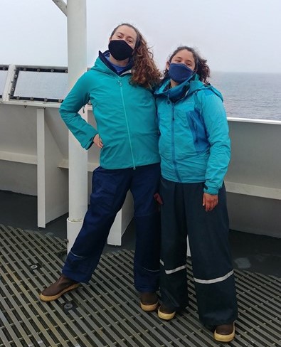
Dawn and Rachel in matching, many-layered outfits, 125 miles offshore on the flying bridge of the RV Bell M. Shimada.
Run by NOAA, this Northern California Current (NCC) cruise takes place three times per year. It is fabulously interdisciplinary, with teams concurrently conducting research on phytoplankton, zooplankton, seabirds, and more. The GEMM Lab will use the whale survey, krill, and oceanographic data to fuel species distribution models as part of Project OPAL. I’ll be working with this data for my PhD, and it’s great to be getting to know the region, study system, and sampling processes.
I’ve been to sea a number of times and always really enjoyed it, but this is my first time as part of a marine mammal survey. The type and timing of this work is so different from the many other types of oceanographic science that take place on a typical research cruise. While everyone else is scurrying around, deploying instruments and collecting samples at a “station” (a geographic waypoint in the ocean that is sampled repeatedly over time), we – the marine mammal team – are taking a break because we can only survey when the boat is moving. While everyone else is sleeping or relaxing during a long transit between stations, we’re hard at work up on the flying bridge of the ship, scanning the horizon for animals.
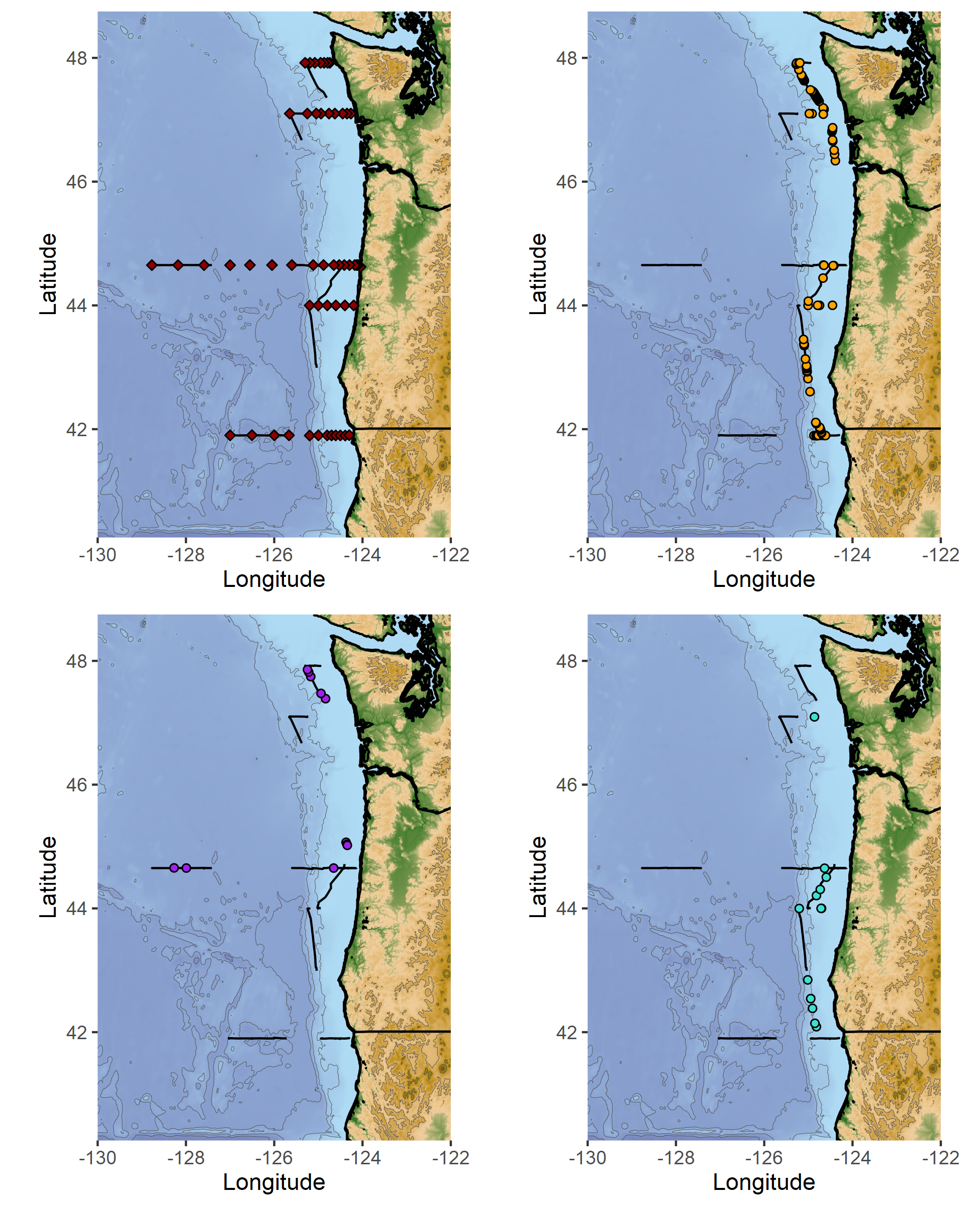
Top left: marine mammal survey effort (black lines), and oceanographic sampling stations (red diamonds). Top right: humpback whale sighting locations. Bottom left: fin whale sighting locations. Bottom right: pacific white-sided dolphin sighting locations.
During each “on effort” survey period, Dawn and I cover separate quadrants of ocean, each manning either the port or starboard side. We continuously scan the horizon for signs of whale blows or bodies, alternating between our eyes and binoculars. During long transits, we work in chunks – forty minutes on effort, and twenty minutes off effort. Staring at the sea all day is surprisingly tiring, and so our breaks often involve “going to the eye spa,” which entails pulling a neck gaiter or hat over your eyes and basking in the darkness.
Dawn has been joining these NCC cruises for the last four years, and her wealth of knowledge has been a great resource as I learn how to survey and identify marine mammals. Beyond learning the telltale signs of separate species, one of the biggest challenges has been learning how to read the sea better, to judge the difference between a frothy whitecap and a whale blow, or a distant dark wavelet and a dorsal fin. Other times, when conditions are amazing and it feels like we’re surrounded by whales, the trick is to try to predict the positions and trajectory of each whale so we don’t double-count them.
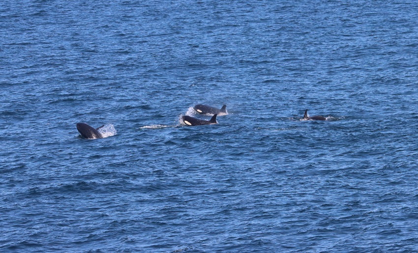
Over the last week, all our scanning has been amply rewarded. We’ve seen pods of dolphins play in our wake, and spotted Dall’s porpoises bounding alongside the ship. Here on the Heceta Line, we’ve seen a diversity of pinnipeds, including Northern fur seals, Stellar sea lions, and California sea lions. We’ve been surprised by several groups of fin whales, farther offshore than expected, and traveled alongside a pod of about 12 orcas for several minutes, which is exactly as magical as it sounds.
Killer whales traveling alongside the Bell M. Shimada, putting on a show for the NCC science team and ship crew. Photo by Dawn Barlow.
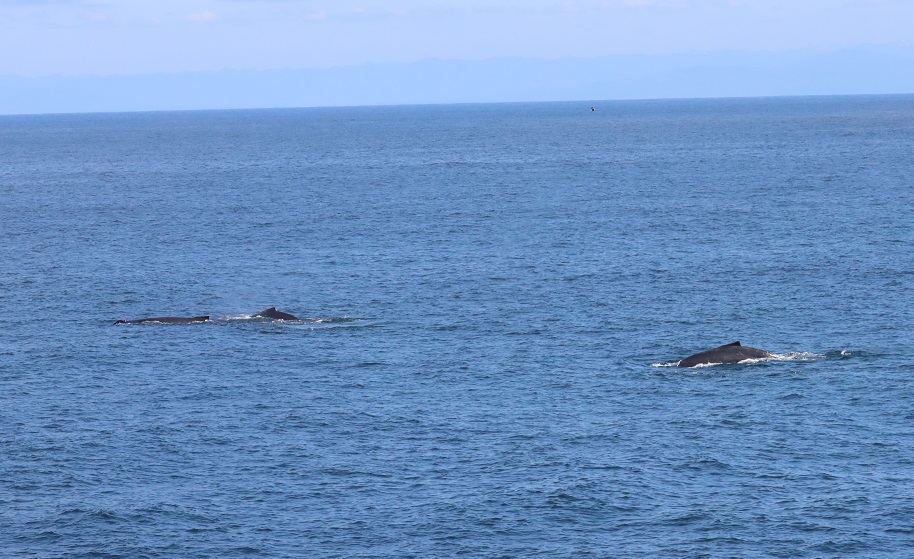
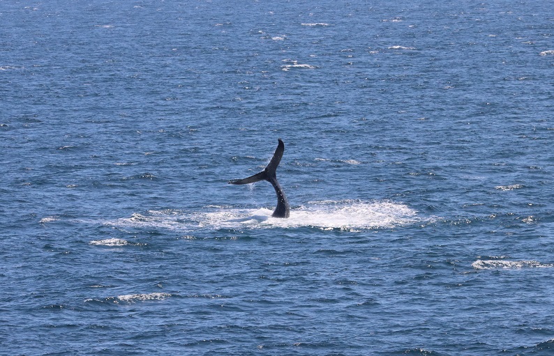
Notably, we’ve also seen dozens of humpbacks, including along what Dawn termed “the humpback highway” during our transit offshore of southern Oregon. One humpback put on a huge show just 200 meters from the ship, demonstrating fluke slapping behavior for several minutes. We wanted to be sure that everyone onboard could see the spectacle, so we radioed the news to the bridge, where the officers control the ship. They responded with my new favorite radio call ever: “Roger that, we are currently enamored.”
A group of humpbacks traveling along the humpback highway. Photo by Dawn Barlow.A humpback whale fluke slapping. Photo by Dawn Barlow.
Even with long days and tired eyes, we are still constantly enamored as well. It has been such a rewarding cruise so far, and it’s hard to think of returning back to “real life” next week. For now, we’re wishing you the same things we’re enjoying – great weather, unlimited coffee, and lots of whales!
The ocean is vast, ever-changing, and at first glance, seemingly featureless. Yet, we know that the warm, blue tropics differ from icy polar waters, and that temperate kelp forests are different from coral reefs. In the connected fluid environment of the global oceans, how do such different habitats exist, and what separates them? On a smaller scale, you may observe a current mixing line at the ocean surface, or dive down from the surface and feel the temperature drop sharply. In a featureless ocean, what boundaries exist, and how can we delineate between different environments?
These questions have been on my mind recently as I study for my PhD Qualifying Exams, an academic milestone that involves written and oral exams prepared by each committee member for the student. The subject matter spans many different areas, including ecological theory, underwater acoustics, oceanography, zooplankton dynamics, climate change and marine heatwaves, and protected area design. Yet, in my recent studying, I was struck by a realization: since when did my PhD involve so much physics? Atmospheric pressure differences generate wind, which drive global ocean circulation patterns. Density properties of seawater create structure in the ocean, and these physical features influence productivity and aggregate prey for predators such as whales. Sound propagates through the fluid ocean as a pressure wave, and its transmission is influenced by physical characteristics of the sound and the medium it moves through. Many of these examples can be distilled and described with equations rooted in physics. Physics doesn’t behave, it simply… is. In considering the vast and dynamic ocean, there is something quite satisfying in that simple notion.
Circling back to boundaries in the ocean, there are changes in physical properties of the oceans that create boundaries, some stark and some nuanced. These physical features structure and partition the marine environment through differences in properties such as temperature, salinity, density, and pressure. Geographic partitions can occur in both horizontal and vertical dimensions of the water column, and on scales ranging from less than a kilometer to thousands of kilometers [1,2].
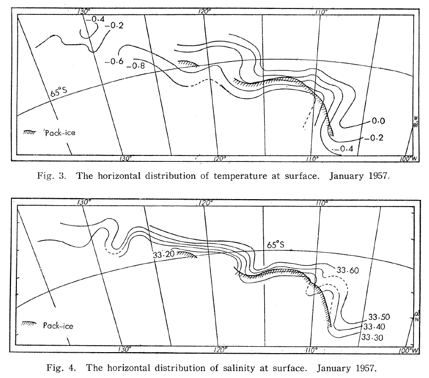
In the horizontal dimension, currents, fronts, and eddies mark transition zones between environments. In the time of industrial whaling, observations of temperature and salinity were made at the surface from factory whaling ships and examined to understand where the most whales were available for hunting. These early measurements identified temperature contour lines, or isotherms, and led to observations that whales were found in areas of stark temperature change and places where isotherms bent into “tongues” of interacting water masses [3,4] (Fig. 1). These areas where water masses of different properties meet are often areas of high productivity. Today, we understand that shelf break fronts, river plumes, tidal fronts, and eddies are important horizontal structures that drive elevated nutrient availability, phytoplankton production, and prey availability for mobile marine predators, including whales.
Figure 1. Surface temperature and salinity contour lines from measurements taken aboard a factory whaling ship in the Antarctic, reproduced from Nasu (1959).
In the vertical dimension, the water column is also structured into distinct layers. Surface waters are warmed by the sunlight and are often lower in salinity due to freshwater input from rain and runoff. Below this distinct surface portion of the water column, the temperature drops sharply in a layer known as the thermocline, and below which pressure and density increase with depth. The surface layer is subject to mixing from wind input, which can draw nutrients from below up into the photic zone and spur productivity. The alternation between stratification—a water column with distinctive layers—and mixing drives optimal conditions for entire food webs to thrive [1,2].
While I began this blog post by writing about boundaries that partition different ocean environments, I have continued to learn that those boundary zones are often critically important in their own right. I started by thinking about boundaries in terms of their importance for separation, but now understand that the leaky points between them actually spur ocean productivity. Features such as fronts, currents, mixed layers, and eddies separate water masses of different properties. However, they are not truly complete and rigid boundaries, and precisely for that reason they are uniquely important in promoting productive marine ecosystems.
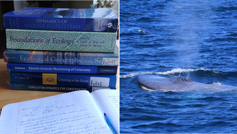
Figure 2. Left: Some of the materials I am studying for my qualifying exams. Right: A blue whale surfaces in New Zealand’s South Taranaki Bight, the subject of my PhD and the lens through which I consider the concepts I am reading about (photo by L. Torres).
Many thanks to my PhD Committee members who continue to guide me through this degree and who I am lucky to learn from. In particular, the contents of this blog post were inspired by materials recommended by, and discussions with, Dr. Daniel Palacios.
References:
1. Mann, K.H., and Lazier, J.R.N. (2006). Dynamics of Marine Ecosystems 3rd ed. (Blackwell Publishing).
2. Longhurst, A.R. (2007). Ecological Geography of the Sea 2nd ed. (Academic Press).
3. Nasu, K. (1959). Surface water conditions in the Antarctic whaling pacific area in 1956-57.
4. Machida, S. (1974). Surface temperature fields in the Crozet and Kerguelen whaling grounds. Sci. Reports Whales Res. Inst. 26, 271–287.
Knowing what and how much prey a predator feeds on are key components to better understanding and conserving that predator. Prey abundance and availability are frequently predictors for marine predator reproductive success and population dynamics. It is the reason why the GEMM Lab makes a concerted effort to not only track our main taxa of interest (marine mammals) but to simultaneously measure their prey. However, over the last decade or two, there has been increased recognition that prey quality is also highly important in understanding a predator’s ecology (Spitz et al. 2012). Optimal foraging theory is a widely accepted framework that posits that predators should attempt to maximize energy gained and minimize energy spent during a foraging event (Charnov 1976, Krebs 1978, Pyke 1984). Thus, knowledge of how valuable a prey item is in terms of its energetic content is an important part of the equation when applying optimal foraging theory to a predator of interest.
Ideally, the prey species with the highest energetic value would also be the easiest, most ubiquitous and least energetically expensive prey item to capture and consume, such that a predator truly could expend very little energy to get very high energetic rewards. However, it rarely is this straightforward. The caloric content of several marine prey species has been shown to increase with increasing size (e.g. Benoit-Bird 2004; Fig. 1), both length and weight. Yet, increasing size often also means increased mobility and, as a result, ability to evade and escape predation. Furthermore, increasing size also inherently means decreasing abundances – there will always be billions more krill in the ocean than whales based solely on cost of reproduction. Therefore, just based on sheer numbers, there are fewer big prey items, which increases the time between, and decreases the likelihood of, a predator encountering big prey items. So, there are clear trade-offs here. It may take longer to locate and capture a high value prey item, which costs more energy to capture, but the payout could potentially be much bigger. However, if a predator gambles too much, then their net energy expenditure to obtain high value prey may be higher than the net energy gained. Instead, it may be worth pursuing smaller prey items with lower energetic values, where discovery and capture success are higher and more frequent. However, in this case, many, many more pursuits are likely needed, thus costing more energy to meet daily energetic demands.
Figure 1. Increasing caloric content with increasing length (a) and wet weight (b). Figures and caption reproduced from Benoit-Bird 2004.
Is your head spinning as much as mine? Let me try and simplify this complex web of interactions with a tangible example. Bowen et al. (2002) investigated foraging of harbor seals in Nova Scotia to assess prey profitability of different species. By attaching camera systems to the backs of 39 adult male harbor seals, the authors identified sand lance and flounder to be the most targeted prey species. However, there were significant differences in pursuit/handling cost per prey type (kJ/min) with sand lance only requiring 14.8 ± 2.7, whereas flounder required significantly more at 30.3 ± 7.9. Therefore, based solely on energy required to capture prey, the sand lance would seem to be the better option. In fact, to a certain degree, this hypothesis is actually true when we compare the energetic content of the two prey types. Sand lance have a higher energetic value at lengths of 10 and 15 cm (53.6 and 95.8 kJ, respectively) compared to flounder (22.6 and 88.6 kJ, respectively). So, the net gain of a harbor seal foraging on a 15 cm sand lance (assuming that it only takes 1 minute to catch the fish – this is more for explanatory purposes as it likely takes much longer for a harbor seal to capture a fish) would be 81 kJ. This gain is larger than that of a 15 cm flounder (58.3 kJ). However, once we compare these fish at 20 and 25 cm lengths, the flounder actually becomes the more beneficial prey item at 232.6 and 492.3 kJ, respectively, over the sand lance (158.1 and 233.8 kJ). Now, assuming once again that it only takes 1 minute to catch the fish, the harbor seal enjoys a net energetic gain of a whopping 462 kJ when capturing a 25 cm flounder compared to 219 kJ for a sand lance of the same size – that makes the flounder more than twice as profitable!
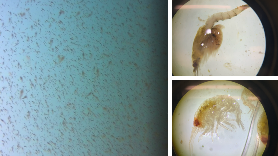
The Bowen et al. study is an excellent demonstration of the importance of considering the quality of prey items when studying the ecology of marine predators. However, the authors did not assess the relative availability of sand lance and flounder. Ideally, foraging ecology studies aimed at understanding prey choice would try to address both important prey metrics – quality and quantity. This goal is the exact aim of my second Master’s thesis chapter where I am investigating whether prey quality (determined through community composition and caloric content) or prey quantity (measured as relative density) is more important in driving fine-scale gray whale foraging behavior in Port Orford, Oregon (Fig. 2). This question can be simplified by asking does it matter more what prey is in an area, or how much prey there is in an area? Or we can relate it back to the title of this post by asking whether individual gray whales would rather attend a cheap all-you-can-eat buffet or an expensive fine-dining restaurant. I am unfortunately not quite done with my analyses yet (but I’m getting closer!) and therefore am not ready to answer these questions. However, I have done extensive research on this topic and therefore am in a position to briefly mention a few other studies that have investigated these questions for other marine predators.
Figure 2. A question of what or how much. Left image: example of the screenshots we take to estimate relative prey density in Port Orford. Right images: two examples of the main prey species we find (top: mysid shrimp Neomysis rayii with a full brood pouch; bottom: amphipod Polycheria osborni).
Ludynia et al. (2010) explored reasons why African penguin (Spehniscus demersus) numbers have declined in Namibia. They found that after the collapse of pelagic fish stocks in the 1970s (including the principal penguin prey item, sardine), African penguins switched to feeding on bearded goby, which are considered a low-energy prey species. Bearded goby are relatively abundant along Namibia’s southern coast and as such, limited prey availability is not the reason for declining African penguin numbers. Therefore, the authors concluded that the low quality of bearded goby (compared to sardine) appears to be the reason for declining population trends of the penguins. This study demonstrates that African penguins do better when eating at a fine-dining restaurant, rather than loading up a whole plate of junk food.
Grémillet et al. (2004) studied the foraging effort and number of successful prey captures per foraging trip (yield) of great cormorants (Phalacrocorax carbo) in Greenland in relation to prey abundance and quality within their foraging areas. The authors radio-tracked 11 great cormorants during a total of 163 foraging trips to estimate foraging effort and yield. The study found that contrary to the authors’ hypothesis, great cormorants foraged in areas of low prey abundance where the average caloric value was also relatively low. Therefore, in this example, it would seem that the predator of interest prioritizes neither high quality nor quantity when foraging.
Haug et al. (2002) investigated the variations in minke whale (Balaenoptera acutorostrata) diet and body condition in response to ecosystem changes in the Barents Sea. The main prey item of minke whales in the Barents Sea is immature herring. However, when recruitment failure and subsequent weak cohorts leads to reduced availability of immature herring, minke whales switched their diet to other prey items such as krill, capelin, and sometimes other gadoid fish species. The authors found a correlation between body condition of minke whales and immature herring abundances, such that minke whales displayed a poor body condition during low immature herring abundances. However, in the years of low immature herring abundance, abundances of krill and capelin were not low. Therefore, similar to the Ludynia et al. (2010) study, it seems that minke whales in the Barents Sea also do better in years when the prey type of highest caloric value is the most abundant. However, decreases in high quality prey has not led to population declines in minke whales in the Barents Sea, indicating that they likely take advantage of high quantities of low quality prey, unlike the African penguins.
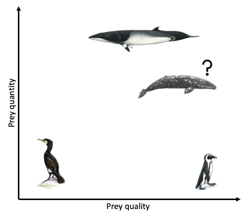
Clearly, the answer as to whether marine predators prefer quality over quantity is not simple and constant. Rather, prey preference varies based on predator needs and ecology, falling anywhere on a broad spectrum from low to high prey quality and low to high prey quantity (Fig. 3). To a certain extent, it probably also is not solely predator choice that determines what they eat but many other factors, such as climate, disturbance, and health. As a result, these preferences and choices will likely be fluid, rather than fixed. While I anticipate that individual gray whales will be flexible foragers, I do hypothesize that when there is a prey patch of a higher energetic value in the area, whales will preferentially consume these patches over areas where there is less energetically rich prey, even if it is more abundant.
Figure 3. A spectrum of prey quantity and quality. Giant cormorants forage on low prey quality & quantity (Grémillet et al. 2004). African penguin populations are declining despite high abundances of low quality prey, suggesting that high prey quality is important for their survival (Ludynia et al. 2010). Body condition of Barents Sea minke whales decreases when high quality prey is less abundant, however their populations have not declined, suggesting they instead exploit high abundances of low quality prey (Haug et al. 2002). What will the gray whales do?
Literature cited
Benoit-Bird, K. J. 2004. Prey caloric value and predator energy needs: foraging predictions for wild spinner dolphins. Marine Biology 145:435-444.
Bowen, W. D., D. Tuley, D. J. Boness, B. M. Bulheier, and G. J. Marshall. 2002. Prey-dependent foraging tactics and prey profitability in a marine mammal. Marine Ecology Progress Series 244:235-245.
Charnov, E. L. 1976. Optimal foraging, the marginal value theorem. Theoretical Population Biology 9(2):129-136.
Grémillet D., G. Kuntz, F. Delbart, M. Mellet, A. Kato, J-P. Robin, P-E. Chaillon, J-P. Gendner, S-H. Lorentsen, and Y. Le Maho. 2004. Linking the foraging performance of a marine predator to local prey abundance. Functional Ecology 18(6):793-801.
Haug, T., U. Lindstrøm, and K. T. Nilssen. 2002. Variations in minke whale (Balaenoptera acutorostrata) diet and body condition in response to ecosystem changes in the Barents Sea. Sarsia 87(6):409-422.
Krebs, J. R. 1978. Optimal foraging: decision rules for predators. Behvaioral Ecology: An Evolutionary Approach, eds. Krebs, J. R., and N. B. Davies. Oxford: Blackwell.
Ludynia, J., J-P. Roux, R. Jones, J. Kemper, and L. G. Underhill. 2010. Surviving off junk: low-energy prey dominates the diet of African penguins Spheniscus demersus at Mercury Island, Namibia, between 1996 and 2009. African Journal of Marine Science 32(3):563-572.
Pyke, G. H. 1984. Optimal foraging theory: a critical review. Annual Reviews of Ecology and Systematics 15:523-575.
Spitz, J., A. W. Trites, V. Becquet, A. Brind’Amour, Y. Cherel, R. Galois, and V. Ridoux. 2012. Cost of living dictates what whales, dolphins and porpoises eat: the importance of prey quality on predator foraging strategies. PLoS ONE 7(11):e50096.
Young, J. K., B. A. Black, J. T. Clarke, S. V. Schonberg, and K. H. Dunton. 2017. Abundance, biomass and caloric content of Chukchi Sea bivalves and association with Pacific walrus (Odobenus rosmarus divergens) relative density and distribution in the northeastern Chukchi Sea. Deep-Sea Research Part II 144:125-141.
The last two months have been challenging for everyone across the world. While I have also experienced lows and disappointments during this time, I always try to see the positives and to appreciate the good things every day, even if they are small. One thing that I have been extremely grateful and excited about every week is when the clock strikes 9:58 am every Thursday. At that time, I click a Zoom link and after a few seconds of waiting, I am greeted by the smiling faces of the GEMM Lab. This spring term, our Principal Investigator Dr. Leigh Torres is teaching a reading and conference class entitled ‘Cetacean Behavioral Ecology’. Every week there are 2-3 readings (a mix of book chapters and scientific papers) focused on a particular aspect of behavioral ecology in cetaceans. During the first week we took a deep dive into the foundations of behavioral ecology (much of which is terrestrial-based) and we have now transitioned into applying the theories to more cetacean-centric literature, with a different branch of behavior and ecology addressed each week.
Leigh dedicated four weeks of the class to discussing foraging behavior, which is particularly relevant (and exciting) to me since my Master’s thesis focuses on the fine-scale foraging ecology of gray whales. Trying to understand the foraging behavior of cetaceans is not an easy feat since there are so many variables that influence the decisions made by an individual on where and when to forage, and what to forage on. While we can attempt to measure these variables (e.g., prey, environment, disturbance, competition, an individual’s health), it is almost impossible to quantify all of them at the same time while also tracking the behavior of the individual of interest. Time, money, and unworkable weather conditions are the typical culprits of making such work difficult. However, on top of these barriers is the added complication of scale. We still know so little about the scales at which cetaceans operate on, or, more importantly, the scales at which the aforementioned variables have an effect on and drive the behavior of cetaceans. For instance, does it matter if a predator is 10 km away, or just when it is 1 km away? Is a whale able to sense a patch of prey 100 m away, or just 10 m away? The same questions can be asked in terms of temporal scale too.
What is that gray whale doing in the kelp? Source: F. Sullivan.
As such, cetacean field work will always involve some compromise in data collection between these factors. A project might address cetacean movements across large swaths of the ocean (e.g., the entire U.S. west coast) to locate foraging hotspots, but it would be logistically complicated to simultaneously collect data on prey distribution and abundance, disturbance and competitors across this same scale at the same time. Alternatively, a project could focus on a small, fixed area, making simultaneous measurements of multiple variables more feasible, but this means that only individuals using the study area are studied. My field work in Port Orford falls into the latter category. The project is unique in that we have high-resolution data on prey (zooplankton) and predators (gray whales), and that these datasets have high spatial and temporal overlap (collected at nearly the same time and place). However, once a whale leaves the study area, I do not know where it goes and what it does once it leaves. As I said, it is a game of compromises and trade-offs.
Ironically, the species and systems that we study also live a life of compromises and trade-offs. In one of this week’s readings, Mridula Srinivasan very eloquently starts her chapter entitled ‘Predator/Prey Decisions and the Ecology of Fear’ in Bernd Würsig’s ‘Ethology and Behavioral Ecology of Odontocetes’ with the following two sentences: “Animal behaviors are governed by the intrinsic need to survive and reproduce. Even when sophisticated predators and prey are involved, these tenets of behavioral ecology hold.”. Every day, animals must walk the tightrope of finding and consuming enough food to survive and ensure a level of fitness required to reproduce, while concurrently making sure that they do not fall prey to a predator themselves. Krebs & Davies (2012) very ingeniously use the idea of economic analysis of costs and benefits to understand foraging behavior (but also behavior in general). While foraging, individuals not only have to assess potential risk (Fig. 1) but also decide whether a certain prey patch or item is profitable enough to invest energy into obtaining it (Fig. 2).
Leigh’s class has been great, not only to learn about foundational theories but to then also apply them to each of our study species and systems. It has been exciting to construct hypotheses based on the readings and then dissect them as a group. As an example, Sih’s 1984 paper on the behavioral response race of predators and prey prompted a discussion on responses of predators and prey to one another and how this affects their spatial distributions. Sih posits that since predators target areas with high prey densities, and prey will therefore avoid areas that predators frequent, their responses are in conflict with one another. Resultantly, there will be different outcomes depending on whichever response dominates. If the predator’s response dominates (i.e. predators are able to seek out areas of high prey density before prey can respond), then predators and prey will have positively correlated spatial distributions. However, if the prey responses dominate, then the spatial distributions of the two should be negatively correlated, as predators will essentially always be ‘one step behind’ the prey. Movement is most often the determinant factor to describe the strength of these relationships.
Video 1. Zooplankton closest to the camera will jump or dart away from it. Source: GEMM Lab.
So, let us think about this for gray whales and their zooplankton prey. The latter are relatively immobile. Even though they dart around in the water column (I have seen them ‘jump’ away from the GoPro when we lower it from the kayak on several occasions; Video 1), they do not have the ability to maneuver away fast or far enough to evade a gray whale predator moving much faster. As such, the predator response will most likely always be the strongest since gray whales operate at a scale that is several orders of magnitude greater than the zooplankton. However, the zooplankton may not be as helpless as I have made them seem. Based on our field observations, it seems that zooplankton often aggregate beneath or around kelp. This behavior could potentially be an attempt to evade predators as the kelp and reef crevices may serve as a refuge. So, in areas with a lot of refuges, the prey response may in fact dominate the relationship between gray whales and zooplankton. This example demonstrates the importance of habitat in shaping predator-prey interactions and behavior. However, we have often observed gray whales perform “bubble blasts” in or near kelp (Video 2). We hypothesize that this behavior could be a foraging tactic to tip the see-saw of predator-prey response strength back into their favor. If this is the case, then I would imagine that gray whales must decide whether the energetic benefit of eating zooplankton hidden in kelp refuges outweighs the energy required to pursue them (Fig. 2). On top of all these choices, are the potential risks and threats of boat traffic, fishing gear, noise, and potential killer whale predation (Fig. 1). Bringing us back to the analogy of economic analysis of costs and benefits to predator-prey relationships. I never realized it so clearly before, but gray whales sure do have a lot of decisions to make in a day!
Video 2. Drone footage of a gray whale foraging in kelp and performing a “bubble blast” at 00:40. Footage captured under NMFS permit #21678. Source: GEMM Lab.
Trying to tease apart these nuanced dynamics is not easy when I am unable to simply ask my study subjects (gray whales) why they decided to abandon a patch of zooplankton (Were the zooplankton too hard to obtain because they sought refuge in kelp, or was the patch unprofitable because there were too few or the wrong kind of zooplankton?). Or, why do gray whales in Oregon risk foraging in such nearshore coastal reefs where there is high boat traffic (Does their need for food near the reefs outweigh this risk, or do they not perceive the boats as a risk?). So, instead, we must set up specific hypotheses and use these to construct a thought-out and informed study design to best answer our questions (Mann 2000). For the past few weeks, I have spent a lot of time familiarizing myself with spatial packages and functions in R to start investigating the relationships between zooplankton and kelp hidden in the data we have collected over 4 years, to ultimately relate these patterns to gray whale foraging. I still have a long and steep journey before I reach the peak but once I do, I hope to have answers to some of the questions that the Cetacean Behavioral Ecology class has inspired.
Literature cited
Krebs, J. R., and N. B. Davies. 2012. Economic decisions and the individual in Davies, N. B. et al., eds. An introduction to behavioral ecology. John Wiley & Sons, Oxford.
Mann, J. 2000. Unraveling the dynamics of social life: long-term studies and observational methods in Mann, J., ed. Cetacean societies: field studies of dolphins and whales. University of Chicago Press, Chicago.
Sih, A. 1984. The behavioral response race between predator and prey. The American Naturalist 123:143-150.
Srinivasan, M. 2019. Predator/prey decisions and the ecology of fear in Würsig, B., ed. Ethology and ecology of odontocetes. Springer Nature, Switzerland.
1Masters Student in Marine Resource Management, 2Doctoral Student in Integrative Biology
Five years ago, the North Pacific Ocean
experienced a sudden increase in sea surface temperature (SST), known as the
warm blob, which altered marine ecosystem function and structure (Leising et
al. 2015). Much research illustrated how the warm blob impacted pelagic
ecosystems, with relatively less focused on the nearshore environment. Yet, a
new study demonstrated how rising ocean temperatures have partially led to
bull kelp loss in northern California. Unfortunately, we are once again observing
similar warming trends, representing the second largest marine heatwave
over recent decades, and signaling the potential rise of a second warm blob. Taken
together, all these findings could forecast future warming-related ecosystem
shifts in Oregon, highlighting the need for scientists and managers to consider
strategies to prevent future kelp loss, such as reintroducing sea otters.
In northern California, researchers observed a dramatic
ecosystem shift from productive bull kelp forests to purple sea urchin barrens.
The study, led by Dr. Laura Rogers-Bennett from the University of California,
Davis and California Department of Fish and Wildlife, determined that this
shift was caused by multiple climatic and biological stressors. Beginning in
2013, sea star populations were decimated by sea star wasting
disease (SSWD). Sea stars are a main predator of urchins, causing their
absence to release purple urchins from predation pressure. Then, starting in
2014, ocean temperatures spiked with the warm blob. These two events created
nutrient-poor conditions, which limited kelp growth and productivity, and allowed
purple urchin populations to grow unchecked by predators and increase grazing
on bull kelp. The combined effect led to approximately 90% reductions in bull
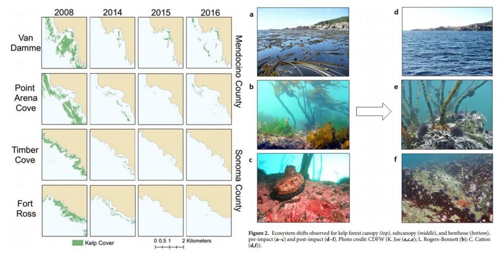
kelp, with a reciprocal 60-fold increase in purple urchins (Figure 1).
Figure 1. Kelp loss and ecosystem shifts in northern California (Rogers-Bennett & Catton 2019).
These changes have wrought economic challenges as
well as ecological collapse in Northern California. Bull kelp is important habitat
and food source for several species of economic importance including red
abalone and red sea urchins (Tegner & Levin 1982). Without bull kelp, red
abalone and red sea urchin populations have starved, resulting in the subsequent
loss of the recreational red abalone ($44 million) and commercial red sea
urchin fisheries in Northern California. With such large kelp reductions,
purple urchins are also now in a starved state, evidenced by noticeably smaller
gonads (Rogers-Bennett & Catton 2019).
Biogeographically, southern Oregon is very similar
to northern California, as both are composed of complex rocky substrates and
shorelines, bull kelp canopies, and benthic macroinvertebrates (i.e. sea
urchins, abalone, etc.). Because Oregon was also impacted by the 2014-2015 warm
blob and SSWD, we might expect to see a similar coastwide kelp forest loss
along our southern coastline. The story is more complicated than that, however.
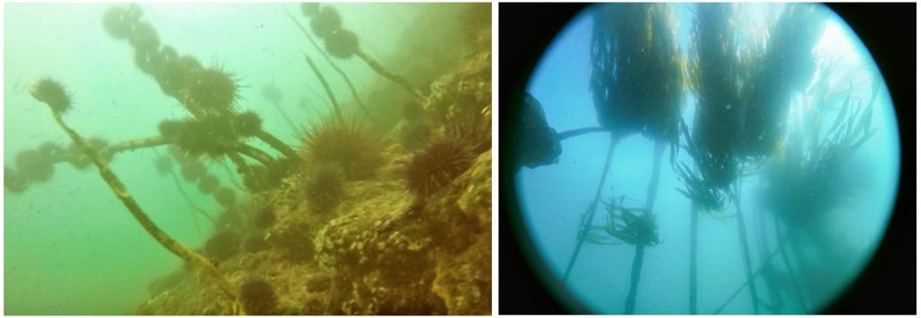
For instance, ODFW
has found purple urchin barrens where almost no kelp remains in some
localized places. The GEMM Lab has video footage of purple urchins climbing up
kelp stalks to graze within one of these barrens near Port Orford, OR (Figure 2,
left). In her study, Dr. Rogers-Bennett explains that this aggressive sea
urchin feeding strategy is potentially a sign of food limitation, where
high-density urchin populations create intense resource competition. Conversely,
at sites like Lighthouse Reef (~45 km from Port Orford) outside Charleston, OR,
OSU and University of Oregon divers are currently seeing flourishing bull kelp
forests. Urchins at this reef have fat, rich gonads, which is an indicator of
high-quality nutrition (Figure 2, right).
Satellites can detect kelp on the surface of the
water, giving scientists a way to track kelp extent over time. Preliminary
results from Sara Hamilton’s Ph.D. thesis research finds that while some kelp
forests have shrunk in past years, others are currently bigger than ever in the
last 35 years. It is not clear what is driving this spatial variability in
urchin and kelp populations, nor why southern Oregon has not yet faced the same
kind of coastwide kelp forest collapse as northern California. Regardless, it
is likely that kelp loss in both northern California and southern Oregon may be
triggered and/or exacerbated by rising temperatures.
Figure 2. Left: Purple urchin aggressive grazing near Port Orford, OR (GEMM Lab 2019). Right: Flourishing bull kelp near Charleston, OR (Sara Hamilton 2019).
The reintroduction of sea otters has been proposed
as a solution to combat rising urchin populations and bull kelp loss in Oregon.
From an ecological perspective, there is some validity to this idea. Sea otters
are a voracious urchin predator that routinely reduce urchin populations and
alleviate herbivory on kelp (Estes & Palmisano 1974). Such restoration and
protection of bull kelp could help prevent red abalone and red sea urchin starvation.
Additionally, restoring apex predators and increasing species richness is often
linked to increased ecosystem resilience, which is particularly important in
the face of global anthropogenic change (Estes et al. 2011)
While sea otters could alleviate grazing pressure
on Oregon’s bull kelp, this idea only looks at the issue from a top-down, not bottom-up,
perspective. Sea otters require a lot of food (Costa 1978, Reidman & Estes
1990), and what they eat will always be a function of prey availability and
quality (Ostfeld 1982). Just because urchins are available, doesn’t mean otters
will eat them. In fact, sea otters prefer large and heavy (i.e. high gonad
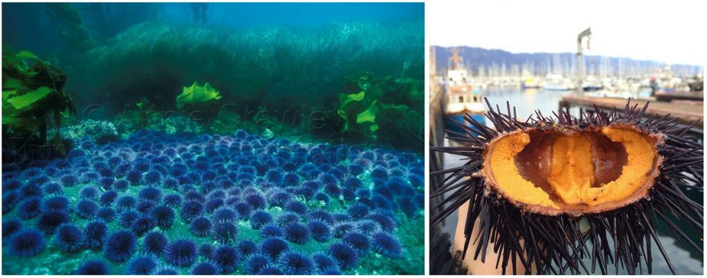
content) urchins (Ostfeld 1982). In the field, researchers have observed sea
otters avoiding urchins at the center of urchin barrens (personal
communication), presumably because those urchins have less access to kelp beds than
on the barren periphery, and therefore, are constantly in a starved state (Konar
& Estes 2003) (Figure 3). These findings suggest prey quality is more
important to sea otter survival than just prey abundance.
Purple urchin quality has not been widely assessed
in Oregon, but early results show that gonad size varies widely depending on
urchin density and habitat type. In places where urchin barrens have formed,
like Port Orford, purple urchins are likely starving and thus may be a poor
source of nutrition for sea otters. Before we decide whether sea otters are a
viable tool to combat kelp loss, prey surveys may need to be conducted to
assess if a sea otter population could be sustained based on their caloric
requirements. Furthermore, predictions of how these prey populations may change
due to rising temperatures could help determine the potential for sea otters to
become reestablished in Oregon under rapid environmental change.
Recent events in California could signal
climate-driven processes that are already impacting some parts of Oregon and could
become more widespread. Dr. Rogers-Bennett’s study is valuable as she has quantified
and described ecosystem changes that might occur along Oregon’s southern
coastline. The resurgence of a potential second warm blob and the frequency
between these warming events begs the question if such temperature spikes are
still anomalous or becoming the norm. If the latter, we could see more
pronounced kelp loss and major shifts in nearshore ecosystem baselines, where function
and structure is permanently altered. Whether reintroducing sea otters can
prevent these changes will ultimately depend on prey and habitat availability
and quality, and should be carefully considered.
References:
Costa, D. P. 1978. The ecological energetics,
water, and electrolyte balance of the California sea otter (Enhydra lutris).
Ph.D. dissertation, University of California, Santa Cruz.
Estes, J. A. and J.F. Palmisano. 1974. Sea
otters: their role in structuring nearshore communities. Science. 185(4156):
1058-1060.
Estes et al. 2011. Trophic downgrading of planet Earth. Science. 333(6040): 301-306.
Harvell et al. 2019. Disease epidemic and a
marine heat wave are associated with the continental-scale collapse of a
pivotal predator (Pycnopodia helianthoides). Science Advances.
5(1).
Konar, B., and J. A. Estes. 2003. The stability of
boundary regions between kelp beds and deforested areas. Ecology. 84(1):
174-185.
Leising et al. 2015. State of California Current
2014-2015: impacts of the warm-water “blob”. CalCOFI Reports. (56):
31-68.
Ostfeld, R. S. 1982. Foraging strategies and prey
switching in the California sea otter. Oecologia. 53(2):
170-178.
Reidman, M. L. and J. A. Estes. 1990. The sea
otter (Enhydra lutris): behavior, ecology, and natural history. United
States Department of the Interior, Fish and Wildlife Service, Biological
Report. 90: 1-126.
Rogers-Bennett, L., and C. A. Catton. 2019. Marine
heat wave and multiple stressors tip bull kelp forest to sea urchin barrens. Scientific
Reports. 9:15050.
Tegner, M. J., and L. A. Levin. 1982. Do sea
urchins and abalones compete in California? International Echinoderms
Conference, Tampa Bay. J. M Lawrence, ed.