We are almost halfway through June which means summer has arrived! Although, here on the Oregon coast, it does not entirely feel like it. We have been swinging between hot, sunny days and cloudy, foggy, rainy days that are reminiscent of those in spring or even winter. Despite these weather pendulums, the GEMM Lab’s GRANITE project is off to a great start in its 8th field season! The field team has already ventured out onto the Pacific Ocean in our trusty RHIB Ruby on four separate days looking for gray whales and in this blog post, I am going to share what we have seen so far.
The core GRANITE field team before the May 24th “trial run”. From left to right: Leigh Torres, KC Bierlich, Clara Bird, Lisa Hildebrand, Alejandro Fernández Ajó. Source: L. Torres.
PI Leigh, PhD candidate Clara and I headed out for a “trial run” on May 24th. While the intention for the day was to make sure all our gear was running smoothly and we still remembered how to complete the many tasks associated with our field work (boat loading and trailering, drone flying and catching, poop scooping, data download, to name a few), we could not resist surveying our entire study range given the excellent conditions. It was a day that all marine field scientists hope for – low winds (< 5 kt all day) and a 3 ft swell over a long period. Despite surveying between Waldport and Depoe Bay, we only encountered one whale, but it was a whale that put a smile on each of our faces. After “just” 252 days, we reunited with Solé, the star of our GRANITE dataset, with record numbers of fecal samples and drone flights collected. This record is due to what seems to be a strong habitat or foraging tactic preference by Solé to remain in a relatively small spatial area off the Oregon coast for most of the summer, rather than traveling great swaths of the coast in search for food. Honest truth, on May 24th we found her exactly where we expected to find her. While we did not collect a fecal sample from her on that day, we did perform a drone flight, allowing us to collect a critical early feeding season data point on body condition. We hope that Solé has a summer full of mysids on the Oregon coast and that we will be seeing her often, getting rounder each time!
Our superstar whale Solé. Her identifying features are a small white line on her left side (green box) and a white dot in front of her dorsal hump on the right side (red circle). Source: GEMM Lab. Photograph captured under NOAA/NMFS permit #21678
Just a week after this trial day, we had our official start to the field season with back-to-back days on the water. On our first day, postdoc Alejandro, Clara and I were joined by St. Andrews University Research Fellow Enrico Pirotta, who is another member of the GRANITE team. Enrico’s role in the GRANITE project is to implement our long-term, replicate dataset into a framework called Population consequences of disturbance (PCoD; you can read all about it in a previous blog). We were thrilled that Enrico was able to join us on the water to get a sense for the species and system that he has spent the last several months trying to understand and model quantitatively from a computer halfway across the world. Luckily, the whales sure showed up for Enrico, as we saw a total of seven whales, all of which were known individuals to us! Several of the whales were feeding in water about 20 m deep and surfacing quite erratically, making it hard to get photos of them at times. Our on-board fish finder suggested that there was a mid-water column prey layer that was between 5-7 m thick. Given the flat, sandy substrate the whales were in, we predicted that these layers were composed of porcelain crab larvae. Luckily, we were able to confirm our hypothesis immediately by dropping a zooplankton net to collect a sample of many porcelain crab larvae. Porcelain crab larvae have some of the lowest caloric values of the nearshore zooplankton species that gray whales likely feed on (Hildebrand et al. 2021). Yet, the density of larvae in these thick layers probably made them a very profitable meal, which is likely the reason that we saw another five whales the next day feeding on porcelain crab larvae once again.
Porcelain crab larvae. Source: GEMM Lab.A happy captain Ale! Source: GEMM Lab.Enrico (right) and myself after collecting a large fecal sample. Source: GEMM Lab.
On our most recent field work day, we only encountered Solé, suggesting that the porcelain crab swarms had dissipated (or had been excessively munched on by gray whales), and many whales went in search for food elsewhere. We have done a number of zooplankton net tows across our study area and while we did collect a good amount of mysid shrimp already, they were all relatively small. My prediction is that once these mysids grow to a more profitable size in a few days or weeks, we will start seeing more whales again.
The GRANITE team from above, waiting & watching for whales, as we will be doing for the rest of the summer! Source: GEMM Lab.
So far we have seen nine unique individuals, flown the drone over eight of them, collected fecal samples from five individuals, conducted 10 zooplankton net tows and seven GoPro drops in just four days of field work! We are certainly off to a strong start and we are excited to continue collecting rock solid GRANITE data this summer to continue our efforts to understand gray whale ecology and physiology.
Literature cited
Hildebrand L, Bernard KS, Torres LGT. 2021. Do gray whales count calories? Comparing energetic values of gray whale prey across two different feeding grounds in the Eastern North Pacific. Frontiers in Marine Science 8. doi: 10.3389/fmars.2021.683634
In September 2020, I was hired as a postdoc in the GEMM Lab and was tasked to conduct the analyses necessary for the OPAL project. This research project has the ambitious, yet essential, goal to fill a knowledge gap hindering whale conservation efforts locally: where and when do whales occur off the Oregon coast? Understanding and predicting whale distribution based on changing environmental conditions is a key strategy to assess and reduce spatial conflicts with human activities, specifically the risk of entanglement in fixed fishing gear.
Starting a new project is always a little daunting. Learning about a new region and new species, in an alien research and conservation context, is a challenge. As I have specialized in data science over the last couple of years, I have been confronted many times with the prospect of working with massive datasets collected by others, from which I was asked to tease apart the biases and the ecological patterns. In fact, I have come to love that part of my job: diving down the data rabbit hole and making my way through it by collaborating with others. Craig Hayslip, faculty research assistant in MMI, was the observer who conducted the majority of the 102 helicopter surveys that were used for this study. During the analysis stage, his help was crucial to understand the data that had been collected and get a better grasp of the field work biases that I would later have to account for in my models. Similarly, it took hours of zoom discussions with Dawn Barlow, the GEMM lab’s latest Dr, to be able to clean and process the 75 days of survey effort conducted at sea, aboard the R/V Shimada and Oceanus.
Once the data is “clean”, then comes the time for modeling. Running hundreds of models, with different statistical approaches, different environmental predictors, different parameters etc. etc. That is when you realize what a blessing it is to work with a supervisor like Leigh Torres, head of the GEMM Lab. As an early career researcher, I really appreciate working with people who help me take a step back and see the bigger picture within which the whole data wrangling work is included. It is so important to have someone help you stay focused on your goals and the ecological questions you are trying to answer, as these may easily get pushed back to the background during the data analysis process.
And here we are today, with the first scientific publication from the OPAL project published, a little more than three years after Leigh and Craig started collecting data onboard the United States Coast Guard helicopters off the coast of Oregon in February 2019. Entitled “Seasonal, annual, and decadal distribution of three rorqual whale species relative to dynamic ocean conditions off Oregon, USA”, our study published in Frontiers in Marine Science presents modern and fine-scale predictions of rorqual whale distribution off Oregon, as well as a description of their phenology and a comparison to whale numbers observed across three decades in the region (Figure 1). This research focuses on three rorqual species sharing some ecological and biological traits, as well as similar conservation status: humpback whales (Megaptera novaeangliae), blue whales (Balaenoptera musculus musculus), and fin whales (Balaenoptera physallus); all of which migrate and feed over the US West coast (see a previous blog to learn more about these species here).
Figure 1: Graphical abstract of our latest paper published in Frontiers in Marine Science.
We demonstrate (1) an increase in rorqual numbers over the last three decades in Oregon waters, (2) differences in timing of migration and habitat preferences between humpback, blue, and fin whales, and (3) predictable relationships of rorqual whale distribution based on dynamic ocean conditions indicative of upwellings and frontal zones. Indeed, these ocean conditions are likely to provide suitable biological conditions triggering increased prey abundance. Three seasonal models covering the months of December-March (winter model), April-July (spring) and August-November (summer-fall) were generated to predict rorqual whale densities over the Oregon continental shelf (in waters up to 1,500 m deep). As a result, maps of whale densities can be produced on a weekly basis at a resolution of 5 km, which is a scale that will facilitate targeted management of human activities in Oregon. In addition, species-specific models were also produced over the period of high occurrence in the region; that is humpback and blue whales between April and November, and fin whales between August and March.
As we outline in our concluding remarks, this work is not to be considered an end-point, but rather a stepping stone to improve ecological knowledge and produce operational outputs that can be used effectively by managers and stakeholders to prevent spatial conflict between whales and human activities. As of today, the models of fin and blue whale densities are limited by the small number of observations of these two species over the Oregon continental shelf. Yet, we hope that continued data collection via fruitful research partnerships will allow us to improve the robustness of these species-specific predictions in the future. On the other hand, the rorqual models are considered sufficiently robust to continue into the next phase of the OPAL project that aims to assess overlap between whale distribution and Dungeness crab fishing gear to estimate entanglement risk.
The curse (or perhaps the beauty?) of species distribution modeling is that it never ends. There are always new data to be added, new statistical approaches to be tested, and new predictions to be made. The OPAL models are no exception to this rule. They are meant to be improved in future years, thanks to continued helicopter and ship-based survey efforts, and to the addition of new environmental variables meant to better predict whale habitat selection. For instance, Rachel Kaplan’s PhD research specifically aims at understanding the distribution of whales in relation to krill. Her results will feed into the more general efforts to model and predict whale distribution to inform management in Oregon.
This first publication therefore paves the way for more exciting and impactful research!
Did you enjoy this blog? Want to learn more about marine life, research, and conservation? Subscribe to our blog and get a weekly message when we post a new blog. Just add your name and email into the subscribe box below.
Reference
Derville, S., Barlow, D. R., Hayslip, C. E., and Torres, L. G. (2022). Seasonal, Annual, and Decadal Distribution of Three Rorqual Whale Species Relative to Dynamic Ocean Conditions Off Oregon, USA. Front. Mar. Sci. 9, 1–19. doi:10.3389/fmars.2022.868566.
Acknowledgments
We gratefully acknowledge the immense contribution of the United State Coast Guard sectors North Bend and Columbia River who facilitated and piloted our helicopter surveys. We would like to also thank NOAA Northwest Fisheries Science Center for the ship time aboard the R/V Bell M. Shimada. We thank the R/V Bell M. Shimada (chief scientists J. Fisher and S. Zeman) and R/V Oceanus crews, as well as the marine mammal observers F. Sullivan, C. Bird and R. Kaplan. We give special recognition and thanks to the late Alexa Kownacki who contributed so much in the field and to our lives. We also thank T. Buell and K. Corbett (ODFW) for their partnership over the OPAL project. We thank G. Green and J. Brueggeman (Minerals Management Service), J. Adams (US Geological Survey), J. Jahncke (Point blue Conservation), S. Benson (NOAA-South West Fisheries Science Center), and L. Ballance (Oregon State University) for sharing validation data. We thank J. Calambokidis (Cascadia Research Collective) for sharing validation data and for logistical support of the project. We thank A. Virgili for sharing advice and custom codes to produce detection functions.
When I was younger, I aspired to be a marine mammal biologist. I thought it was purely about knowing as much about marine mammal species as possible. However, over time and with experience in this field, I have realized that in order to understand a species, you need to have a holistic understanding of its prey, habitat, and environment. When I first applied to be advised by Leigh in the GEMM Lab, I had no idea how much of my time I would spend looking at tiny zooplankton under a microscope, thinking about the different benefits of different habitat types, or reading about oceanographic processes. But these things have been incredibly vital to my research to date and as a result, I now refer to myself as a marine ecologist. This holistic understanding that I am gaining will only grow throughout my PhD as I am broadly looking at the habitat use, site fidelity, and population dynamics of the Pacific Coast Feeding Group (PCFG) of gray whales for my thesis research.
The PCFG display many foraging tactics and occupy several habitat types along the Oregon coast while they spend their summer feeding seasons here (Torres et al. 2018). Here, I will focus on one of these habitats: kelp. When you hear the word kelp, you probably conjure an image of long, thick stalks that reach from the ocean floor to the surface, with billowing fronds waving around (Figure 1a). However, this type is only one of three basic morphologies (Filbee-Dexter & Scheibling 2014) and it is called canopy kelp, which often forms extensive forests. The other two morphologies are stipitate and prostrate kelps. The former forms midwater stands (Figure 1b) while the latter forms low-lying kelp beds (Figure 1c). All three of these morphologies exist on the Oregon coast and create a mosaic of understory and canopy kelp patches that dot our coastline.
Figure 1. Examples of the three different kelp morphologies. a: bull kelp (Nereocystis luetkeana) is a type of canopy kelp and the dominant kelp on the Oregon coast (Source: Oregon Coast Aquarium); b: sea palm (Postelsia palmaeformis) is a type of stipitate kelp that forms mid-water stands (Source: Oregon Conservation Strategy); c: sea cabbage (Saccharina sessilis) is a type of prostrate kelp that is stipeless and forms low-lying kelp beds (Source: Central Coast Biodiversity).
One of the most magnificent things about kelp is that it is not just a species itself, but it provides critical habitat, refuge, and food resources to a myriad of other species due to its high rates of primary production (Dayton 1985). Kelp is often referred to as a foundation species due to all of these critical services it provides. In Oregon, many species of rockfish, which are important commercial and recreational fisheries, use kelp as habitat throughout their life cycle, including as nursery grounds. Lingcod, another widely fished species, forages amongst kelp. A large number of macroinvertebrates can be found in Oregon kelp forests, including anemones, limpets, snails, sea urchins, sea stars, and abalone, to name a fraction of them.
Kelps grow best in cold, nutrient-rich waters (Tegner et al. 1996) and their growth and distribution patterns are highly naturally variable on both temporal and spatial scales (Krumhansl et al. 2016). However, warm water, low nutrient or light conditions, intensive grazing by herbivores, and severe storm activity can lead to the erosion and defoliation of kelp beds (Krumhansl et al. 2016). While these events can occur naturally in cyclical patterns, the frequency of several of these events has increased in recent years, as a result of climate change and anthropogenic impacts. For example, Dawn’s blog discussed increasing marine heatwaves that represent an influx of warm water for a prolonged period of time. In fact, kelps can be useful sentinels of change as they tend to be highly responsive to changes in environmental conditions (e.g., Rogers-Bennet & Catton 2019) and their nearshore, coastal location directly exposes them to human activities, such as pollution, harvesting, and fishing (Bennett et al. 2016).
Due to its foundational role, changes or impacts to kelp can reverberate throughout the ecosystem and negatively affect many other species. As mentioned previously, kelp is naturally highly variable, and like many other ecological processes, undergoes boom and bust cycles. For over four decades, dense, productive kelp forests have been shown to transition to sea urchin barrens, and back again, in natural cycles (Sala et al. 1998;Pinnegar et al. 2000;Steneck et al. 2002; Figure 2). These transitions are called phase shifts. In a healthy, balanced kelp forest, sea urchins typically passively feed on detrital plant matter, such as broken off pieces of kelp fronds that fall to the seafloor. A phase shift occurs when the grazing intensity of sea urchins increases, resulting in them actively feeding on kelp stalks and fronds to a point where the kelp in an area can become greatly reduced, creating an urchin barren. Sea urchin grazing intensity can change for a number of reasons, including reduction in sea urchin predators (e.g., sea otters, sunflower sea stars) or poor kelp recruitment events (e.g., due to warm water temperature). Regardless of the reason, the phases tend to transition back and forth over time. However, there is concern that sea urchin barrens may become an alternative stable state of the subtidal ecosystem from which kelp in an area cannot recover (Filbee-Dexter & Scheibling 2014).
Figure 2. Screenshots from GoPro videos from 2016 (left) and 2018 (right) at the same kayak sampling station in Port Orford showing the difference between a dense kelp forest and what appears to be an urchin barren. (Source: GEMM Lab).
For example, in 2014, bull kelp canopy cover in northern California was reduced by >90% and has not shown signs of recovery since (Rogers-Bennet & Catton 2019; Figure 3). This massive decline was attributed to two major events: 1) the onset of sea star wasting disease (SSWD) in 2013 and 2) the “warm blob” of 2014-2016. SSWD affected over 20 sea star species along the coast from Mexico to Alaska, with the predatory sunflower sea star, which consumes purple sea urchins, most affected, including population declines of 80-100% along the coast (Harvell et al. 2019). Following this SSWD outbreak, the “warm blob”, which was an extreme marine heatwave in the Pacific Ocean, caused ocean temperatures to spike. These two events allowed purple sea urchin populations to grow unchecked by their predators, and created nutrient-poor and warm water conditions, which limited kelp growth and productivity. Intense grazing on bull kelp by growing urchin populations resulted in the >90% reduction in bull kelp canopy cover and has left behind widespread urchin barrens instead (Rogers-Bennet & Catton 2019). Consequently, there have been ecological and economic impacts on the ecosystem and communities in northern California. Without bull kelp, red abalone and red sea urchin populations starved, leading to a subsequent loss of the recreational red abalone (estimated value of $44 million/year) and commercial red urchin fisheries in northern California (Rogers-Bennet & Catton 2019).
Figure 3. Surface kelp canopy area pre- and post-impact from sites in Sonoma and Mendocino counties, northern California from aerial surveys (2008, 2014-2016). Figure and figure caption taken from Rogers-Bennett & Catton (2019).
As I mentioned earlier, while phase shifts between kelp forests and urchin barrens are common cycles, the intensity of the events described above in northern California are an example of sea urchin barrens potentially becoming a stable state of the subtidal ecosystem (Filbee-Dexter & Scheibling 2014). Given that marine heatwaves are only expected to increase in intensity and frequency in the future (Frölicher et al. 2018), the events documented in northern California may not be an isolated incidence.
Considering that parts of the Oregon coast, particularly the southern portion, are very similar to northern California biogeographically, and that it was not exempt from the “warm blob”, similar changes in kelp forests may be occurring along our coast. There are many individuals and groups that are actively working on this issue to examine potential impacts to kelp and the species that depend on the services it provides. For more information, check out the Oregon Kelp Alliance.
Figure 4. A gray whale surfaces in a large kelp bed during a foraging bout along the Oregon coast. (Source: GEMM Lab).
So, what does all of this information have to do with gray whales? Given their affinity for kelp habitats (Figure 4) and their zooplankton prey that aggregates there, changes to kelp ecosystems may affect gray whale health and ecology. This aspect of the complex kelp trophic web has not been examined to date; thus one of my PhD chapters focuses on the response of gray whales to changing kelp ecosystems along the southern Oregon coast. To do this, I am examining 6 years of data collected during the TOPAZ/JASPER project in Port Orford, to look at the relationships between kelp health, sea urchin density, zooplankton abundance, and gray whale foraging effort over space and time. Documenting impacts of changing kelp forests on gray whales is important to assist management efforts as healthy and abundant kelp seems critical in providing ample food opportunities for these iconic Pacific Northwest marine predators.
Did you enjoy this blog? Want to learn more about marine life, research, and conservation? Subscribe to our blog and get a weekly alert when we make a new post! Just add your name into the subscribe box on the left panel.
References
Bennett S, et al. The ‘Great Southern Reef’: Social, ecological and economic value of Australia’s neglected kelp forests. Marine and Freshwater Research 67:47-56.
Dayton PK (1985) Ecology of kelp communities. Annual Review of Ecology and Systematics 16:215-245.
Filbee-Dexter K, Scheibling RE (2014) Sea uechin barrens as alternative stable states of collapsed kelp ecosystems. Marine Ecology Progress Series 495:1-25.
Frölicher TL, Fischer EM, Gruber N (2018) Marine heatwaves under global warming. Nature 560:360-364.
Harvell CD, et al. (2019) Disease epidemic and a marine heat wave are associated with the continental-scale collapse of a pivotal predator (Pycnopodia helianthoides). Science Advances 5(1) doi:10.1126/sciadv.aau7042.
Krumhansl KA, et al. (2016) Global patterns of kelp forest change over the past half-century. Proceedings of the National Academy of Sciences of the United States of America 113(48):13785-13790.
Pinnegar JK, et al. (2000) Trophic cascades in benthic marine ecosystems: lessons for fisheries and protected-area management. Environmental Conservation 27:179-200.
Rogers-Bennett L, Catton CA (2019) Marine heat wave and multiple stressors tip bull kelp forest to sea urchin barrens. Scientific Reports 9:15050.
Sala E, Boudouresque CF, Harmelin-Vivien M (1998) Fishing, trophic cascades and the structure of algal assemblages; evaluation of an old but untested paradigm. Oikos 82:425-439.
Steneck RS, et al. (2002) Kelp forest ecosystems: biodiversity, stability, resilience and future. Environmental Conservation 29:436-459.
Tegner MJ, Dayton PK, Edwards PB, Riser KL (1996) Is there evidence for the long-term climatic change in southern California kelp forests? California Cooperative Oceanic Fisheries Investigations Report 37:111-126.
Torres LG, Nieukirk SL, Lemos L, Chandler TE (2018) Drone up! Quantifying whale behavior from a new perspective improves observational capacity. Frontiers in Marine Science doi:10.3389/fmars.2019.00319.
By Allison Dawn, GEMM Lab Master’s student, OSU Department of Fisheries, Wildlife, and Conservation Sciences, Geospatial Ecology of Marine Megafauna Lab
During my second term of graduate school, I have been preparing to write my research proposal. The last two months have been an inspiring process of deep literature dives and brainstorming sessions with my mentors. As I discussed in my last blog, I am interested in questions related to pattern and scale (fine vs. mesoscale) in the context of the Pacific Coast Feeding Group (PCFG) of gray whales, their zooplankton prey, and local environmental variables.
My work currently involves exploring which scales of pattern are important in these trophic relationships and whether the dominant scale of a pattern changes over time or space. I have researched which analysis tools would be most appropriate to analyze ecological time series data, like the impressive long-term dataset the GEMM lab has collected in Port Orford as part of the TOPAZ project, where we have monitored the abundance of whales and zooplankton, as well as environmental variables since 2016.
A useful analytical tool that I have come across in my recent coursework and literature review is called wavelet analysis. Importantly, wavelet analysis can handle non-stationarity and edge detection in time series data. Non-stationarity is when a dataset’s mean and/or variance can change over time or space, and edge detection is the identification of the change location (in time or space). For example, it is not just the cycles or “ups and downs” of zooplankton abundance I am interested in, but when in time or where in space these cycles of “ups and downs” might change in relation to what their previous values, or distances between values, were. Simply stated, non-stationarity is when what once was normal is no longer normal. Wavelet analysis has been applied across a broad range of fields, such as environmental engineering (Salas et al. 2020), climate science (Slater et al. 2021), and bio-acoustics (Buchan et al. 2021). It can be applied to any time series dataset that might violate the traditional statistical assumption of stationarity.
In a recent review of climate science methodology, Slater et al. (2021) outlined the possible behavior of time series data. Using theoretical plots, the authors show that data can a) have the same mean and variance over time, or b) have non-stationarity that can be broken into three major groups – trend, step change, or shifts in variance. Figure 1 further demonstrates the difference between stationary vs. non-stationary data in relation to a given variable of interest over time.
Figure 1. Plots showing the possible magnitude of a given variable across a time series: a) Stationary behavior, b) Non-stationary trend, step-change, and a shift in variance. [Taken from Slater et. al(2021)].
Traditional correlation statistics assumes stationarity, but it has been shown that ecological time series are often non-stationary at certain scales (Cazelles & Hales, 2006). In fact, ecological data rarely meets the requirements of a controlled experiment that traditional statistics require. This non-stationarity of ecological data means that while widely-used methods like generalized linear models and analyses of variances (ANOVAs) can be helpful to assess correlation, they are not always sufficient on their own to describe the complex natural phenomena ecologists seek to explain. Non-stationarity occurs frequently in ecological time series, so it is appropriate to consider analysis tools that will allow us to detect edges to further investigate the cause.
Wavelet analysis can also be conducted across a time series of multiple response variables to assess if these variables share high common power (correlation). When data is combined in this way it is called a cross-wavelet analysis. An interesting paper used cross-wavelet analysis to assess the seasonal response of zooplankton life history in relation to climate warming (Winder et. al 2009). Results from their cross-wavelet analysis showed that warming temperatures over the past two decades increased the voltinism (number of broods per year) of copepods. The authors show that where once annual recruitment followed a fairly stationary pattern, climate warming has contributed to a much more stochastic pattern of zooplankton abundance. From these results, the authors contribute to the hypothesis that climate change has had a temporal impact on zooplankton population dynamics, and recruitment has increasingly drifted out of phase from the original annual cycles.
Figure 2. Cross-wavelet spectrum for immature and adult Leptodiaptomus ashlandi for 1965 through either 2000 or 2005. Plots show a) immatures and temperature, b) adults and temperature, c) immatures and phytoplankton, and d) adults and phytoplankton. Arrows indicate phase between combined time series. 0 degrees is in-phase and 180 degrees is anti-phase. Black contour lines show “cone of influence” or the 95% significance level, every value within the cone is considered significant. Left axis shows the temporal period, and the color legend shows wavelet frequency power, with low frequencies in blue and high frequencies in red. Plots show strong covariation of high common power at the 12-month period until the 1980s. This pattern is especially evident in plot c) and d). [Taken from (Winder et. al 2009)].
While wavelet and cross-wavelet analyses should not be the only tool used to explore data, due to its limitations with significance testing, it is still worth implementing to gain a better understanding of how time series variables relate to each other over multiple spatial and/or temporal scales. It is often helpful to combine multiple methods of analysis to get a larger sense of patterns in the data, especially in spatio-temporal research.
When conducting research within the context of climate change, where the concentration of CO2 in ppm in the atmosphere is a non-stationary time series itself (Figure 3), it is important to consider how our datasets might be impacted by climate change and wavelet analysis can help identify the scales of change.
When considering our ecological time series of data in Port Orford, we want to evaluate how changing ocean conditions may be related to data trends. For example, has the annual mean or variance of zooplankton abundance changed over time, and where has that change occurred in time or space? These changes might have occurred at different scales and might be invisible at other scales. I am eager to see if wavelet analysis can detect these sorts of changes in the abundance of zooplankton across our time series of data, particularly during the seasons of intense heat waves or upwelling.
Did you enjoy this blog? Want to learn more about marine life, research and conservation? Subscribe to our blog and get a weekly email when we make a new post! Just add your name into the subscribe box on the left panel.
References
Buchan, S. J., Pérez-Santos, I., Narváez, D., Castro, L., Stafford, K. M., Baumgartner, M. F., … & Neira, S. (2021). Intraseasonal variation in southeast Pacific blue whale acoustic presence, zooplankton backscatter, and oceanographic variables on a feeding ground in Northern Chilean Patagonia. Progress in Oceanography, 199, 102709.
Cazelles, B., & Hales, S. (2006). Infectious diseases, climate influences, and nonstationarity. PLoS Medicine, 3(8), e328.
Salas, J. D., Anderson, M. L., Papalexiou, S. M., & Frances, F. (2020). PMP and climate variability and change: a review. Journal of Hydrologic Engineering, 25(12), 03120002.
Slater, L. J., Anderson, B., Buechel, M., Dadson, S., Han, S., Harrigan, S., … & Wilby, R. L. (2021). Nonstationary weather and water extremes: a review of methods for their detection, attribution, and management. Hydrology and Earth System Sciences, 25(7), 3897-3935.
Winder, M., Schindler, D. E., Essington, T. E., & Litt, A. H. (2009). Disrupted seasonal clockwork in the population dynamics of a freshwater copepod by climate warming. Limnology and Oceanography, 54(6part2), 2493-2505.
If you are an avid reader of our blog, you probably know quite a bit about gray whales, specifically the Pacific Coast Feeding Group (PCFG) of gray whales. Of the just over 50 GEMM Lab blogs written in 2021, 43% of them were about PCFG gray whales (or at least mentioned gray whales in some way). I guess this statistic is not too surprising when you consider that six of the 10 GEMM Lab members conduct gray whale-related research. You might think that we would have reached our annual limit of online gray whale content with that many blogs featuring these gentle giants, but you would in fact be wrong…
At the end of 2021, we launched a brand new website all about gray whales called IndividuWhale! It features stories of some of the Oregon coast’s most iconic gray whales, as well as information about how we study them, stressors they experience in our waters, and even a game to test your gray whale identification skills. IndividuWhale is a true labor of love that took over a year to create and that we are extremely proud to share with you today. Before I tell you more about the website, I want to take a moment to give a huge shout out to Erik Urdahl who was instrumental in getting this website off the ground and making it as interactive and beautiful as it is – hurrah Erik!
Equal‘s right side with visible boat propeller scars. Source: GEMM Lab.
Like us humans, gray whales have individual personalities and stories. They experience life-altering events, go through periods of stress, must provide for their offspring, and can behave differently to one another. Since Leigh & co. have been conducting in-depth research about PCFG gray whales in Oregon waters since 2016, we have been able to document several fascinating stories and events that these individuals have experienced. Take Equal, for example, a male whale that is at least 7 years old. The GEMM Lab observed Equal on consecutive days in June 2018, where on the first day he looked healthy and normal, but on the second day had fresh boat propeller-like scars on his back. Not only did we document these scars in photographs, but we were also able to collect a fecal sample from Equal the day we observed him with these scars. After analyzing his fecal sample for stress hormones, we discovered that Equal had very high stress levels compared to previous samples collected – unsurprising seeing as he had been hit by a boat! While this event was certainly sad for Equal (although don’t worry – we have seen him many times again in the years after this event looking healthy & normal once again), it was a very fortuitous occurrence for us since we were able to “validate” our stress hormone data relative to the value from Equal when he was clearly stressed out. Find out more about Equal as well as seven other gray whales here!
You might be wondering, how we knew that the whale with the boat propeller scar was Equal and how we recognize him again years after the incident. Gray whales have unique pigmentation patterns on their bodies and flukes that allow us to re-identify individuals between years and distinguish them from one another. Additionally, scars, such as those that Equal now carries on his back, can also be useful in telling whales apart. Therefore, we take photographs of every whale we see to match markings and identify whales. This process is called photo ID. Some individuals can have very distinctive markings, such as Roller Skate who has two big white dots on her right side, while others can look more inconspicuous, like Clouds. Therefore, conducting photo ID requires a lot of attention to detail and perseverance. To learn more about the different features we use to identify individuals, check out the “Studying Whales With Photographs” page. Do you think you have what it takes to tell individuals apart? Then try your luck at our photo ID game after!
Test your photo ID skills in our whale match game!
Unfortunately, these whales do not live in a pristine environment, as is evidenced by Equal’s story. Their main objective during the summer when in Oregon waters is to gain weight (energy stores) by consuming large amounts of prey, which is made more difficult by a number of stressors, including potential fishery entanglements, ocean noise, vessel traffic, and habitat changes. We describe these four stressors on the IndividuWhale website since we are trying to assess the impacts of them on gray whales through our research, however they are certainly not the only stressors that these whales experience. Little is known about the level at which these stressors may have a negative impact on the whales, and how whales react when they experience some of these stressors in concert. The answers to these questions are difficult to tease apart but the GRANITE project is aiming to do so through a framework called Population Consequences of Multiple Stressors (read more about it here). This approach requires a lot of data on a lot of individuals in a population and as you can see from the IndividuWhale website, we are slowly starting to get there! 2022 will certainly bring many more gray whale-themed blogs to this website, and you can share in our journey of learning about the lives of PCFG gray whales by exploring the IndividuWhale website (https://www.individuwhale.com).
Tagging a whale is no easy feat, nor is it without some impact to the whale – no matter how minimized through the use of non-penetrating suction cup tags. Yet, in August 2021 the GEMM Lab initiated a new phase in our research on gray whales, aimed at obtaining a better understanding of the underwater lives and energetics of a gray whale (Figure 1, top image). We captured some amazing data through these specialized, non-invasive tags that provide a brief window into their world and physiology. The video recordings from the tags showed us whales digging their heads into the benthos generating billowing clouds of sediment, likely exploiting desirable prey patches (Figure 1, middle images). We also saw foraging whales undertake dizzying spins and headstands for hours, demonstrating the fascinating maneuverability and flexibility of gray whales (Figure 1, bottom image). But what is motivating us to capture this information?
Figure 1. Top image:One of the suction cup tags attached to the right side of the gray whale “RAT”. Middle images: still images from the video recorded on the tag attached to gray whale “DICE”, where left image depicts the whale “seeing” our research vessel RUBY as “DICE” comes to the surface to breathe, and the right image shows a large sediment cloud generated by “DICE” as it digs its head into the benthos feeding on benthic prey. Bottom image: a visualization of a trackline (grey, blue, & yellow line) of a foraging gray whale (indicated by the blue arrow). The yellow segments depict times during which the whale was on its side or headstanding (suggesting feeding behavior), while the blue segments represent when the whale was traveling or surfacing. You can see how often in the track the whale is presumably feeding based on the amount of yellow segments in the track. Also, note the amount of circular loops the whale performs, displaying the maneuverability of foraging gray whales. Source: GEMM Lab.
The GEMM Lab has researched the ecology and physiology of Pacific Coast Feeding Group (PCFG) gray whales since 2015. Our efforts have filled crucial knowledge gaps to better understand this sub-group of the Eastern North Pacific (ENP) gray whale population. We now know that gray whale body condition increases throughout a foraging season and can fluctuate considerably between years (Soledade Lemos et al. 2020). Additionally, body condition varies significantly by reproductive state, with calves and pregnant females displaying higher body conditions (Soledade Lemos et al. 2020). We have also validated and quantified fecal steroid and thyroid hormone metabolite concentrations, providing us with thresholds to identify a stressed vs. a not stressed whale based on its hormone levels (Lemos et al. 2020). These validations have allowed us to make correlations between poor body condition and the steroid hormone cortisol which confirm that slim whales are stressed, while chubby whales are relaxed (Lemos et al. 2021). These physiological results are particularly salient in the light of our recent findings that PCFG gray whales select prey quality over prey quantity when foraging (Hildebrand et al. in review) and that the caloric content of available prey species in the PCFG range vary significantly (Hildebrand et al. 2021).
While we have addressed several fundamental questions about the PCFG in the last 7 years, answering one question has led to asking 10 more questions – a common pattern in science. Given that we know (1) PCFG whales improve their body condition over the course of the foraging season (Soledade Lemos et al. 2020), (2) PCFG females are able to successfully give birth to and wean calves (Calambokidis & Perez 2017), and (3) certain prey in the PCFG region are of higher caloric value than prey in the ENP Arctic foraging grounds (Hildebrand et al. 2021), a big question that we continue to scratch our heads about is why does the PCFG sub-group have such a small abundance (~250 individuals; Calambokidis et al. 2017) in comparison to the much larger ENP population (~21,000 individuals; Stewart & Weller 2021). Several hypotheses have been suggested including that the energetic costs of feeding may differ between ENP and PCFG whales, with the latter having to expend more energy to obtain prey due to the different foraging behaviors employed (Torres et al. 2018) to obtain diverse prey types, thus justifying the larger abundance of the ENP (Hildebrand et al. 2021).
Quantifying the energetic cost of baleen whale behaviors is not simple. However, the development of animal-borne tags has allowed scientists to make big strides regarding behavioral cost quantification. The majority of this work has focused on rorqual whales (i.e., blue, humpback, fin whales; e.g., Goldbogen et al. 2013; Cade et al. 2016) as their characteristic lunge-feeding strategy produces a distinct signal in the accelerometer sensors integrated within the tags, making feeding events easier to identify. Gray whales, unlike rorquals, do not lunge-feed. ENP gray whales predominantly feed benthically; diving down to the benthos where they turn onto their side and suction mouthfuls of soft sediment (mud) that contains amphipods that they filter out of the mud (Nerini & Oliver 1983). PCFG whales feed benthically as well, but they also use a number of other feeding behaviors to obtain a variety of prey in a variety of benthic habitats, including headstands, bubble blasts, and sharking (Torres et al. 2018). The above-mentioned gray whale feeding behaviors involve much subtler movements than the powerful, distinctive lunges displayed by rorquals, yet they undoubtedly still incur some energetic cost to the whales. However, exactly how energetically costly the various gray whale feeding behaviors are remains unknown.
One of the three suction cup tags we deployed on gray whales. Dr. Cade printed special “kelp shields” (blue part of the tag) to prevent kelp from potentially getting caught underneath the tag since PCFG whales often forage on reefs with a lot of kelp. This tag includes a video camera (the lens can be seen in the center of the tag) to record video of the whale’s underwater behavior. Source: L. Torres.
This knowledge gap is one of the reasons why the GEMM Lab initiated a new project in close collaboration with Dr. Dave Cade from Stanford University and John Calambokidis from Cascadia Research Collective to quantify and understand the energetics and underwater behavior of gray whales using suction-cup tags. The project was kick-started with a very successful pilot effort the week of August 16th this year. Tags were placed on the backs of three different PCFG gray whales with a long carbon fiber pole and attached to the whales with four suction cups. The tags recorded video, position, accelerometry, and magnetometry data, which we will use to recreate the animal’s movements (pitch, roll), heading, trackline, and environment. Although the weather forecast did not look promising for most of the week, we lucked out with perfect conditions for one day during which we managed to deploy three tags on three different gray whales that are well-known, long-term study animals of the GEMM Lab. The tags stayed on the whales for 1-6 hours and were all recovered (including an adventurous trip up the Alsea River which involved a kayak deployment!).
Left: Postdoc Alejandro Ajo Fernandez uses a Yagi antenna to try and locate a tagged whale since the tags have a transmitter that sends a signal when the whale is at the surface to breathe. Right: Dr. Dave Cade proudly showing off the tag that floated up the Alsea River and required a kayak to recover. Source: L. Torres.
Dr. Cade spent the rest of the week teaching GEMM Lab PI Leigh Torres, University of British Columbia Master’s student Kate Colson (who is co-advised by Leigh and Dr. Andrew Trites), and myself the intricacies of data download, processing, and preliminary analysis of the tag data. For her Master’s research, Kate will develop a bioenergetics model for the PCFG sub-group that includes data on foraging energetics (estimated from the tag data) and prey availability in the PCFG foraging range. I plan on using the tag data to assess behavior patterns of PCFG whales relative to habitat as part of my PhD research. All together analysis of the data from these short-term tag deployments will help us get closer to understanding the behavioral choices, habitat needs, and energetic trade-offs of whales living in a rapidly changing ocean. With the success of this pilot effort, we plan to conduct another suction-cup tagging effort next summer to hopefully capture and explore more mysterious underwater behaviors of the PCFG.
An ecstatic team at the end of a very long yet successful day of suction cup tagging. Bottom (from left): Leigh Torres, Lisa Hildebrand, ClaraBird, Dave Cade, KC Bierlich. Top: John Calambokidis.
This project was funded by sales and renewals of the special Oregon whale license plate, which benefits MMI. We gratefully thank all the gray whale license plate holders, who made this research effort possible.
Literature cited
Cade, D. E., Friedlaender, A. S., Calambokidis, J., & Goldbogen, J. A. 2016. Kinematic diversity in rorqual whale feeding mechanisms. Current Biology 26(19):2617-2624. doi:10.1016/j.cub.2016.07.037.
Calambokidis, J., & Perez, A. 2017. Sightings and follow-up of mothers and calves in the PCFG and implications for internal recruitment. IWC Report SC/A17/GW/04 for the Workshop on the Status of North Pacific Gray Whales (La Jolla: IWC).
Calambokidis, J., Laake, J., & Perez, A. 2017. Updated analysis of abundance and population structure of seasonal gray whales in the Pacific Northwest, 1996-2015. IWC Report SC/A17/GW/05 for the Workshop on the Status of North Pacific Gray Whales (La Jolla: IWC).
Goldbogen, J. A., Friedlaender, A. S., Calambokidis, J., McKenna, M. F., Simon, M., & Nowacek, D. P. 2013. Integrative approaches to the study of baleen whale diving behavior, feeding performance, and foraging ecology. BioScience 63(2):90-100. doi:10.1525/bio.2013.63.2.5.
Hildebrand, L., Bernard, K. S., & Torres, L. G. 2021. Do gray whales count calories? Comparing energetic values of gray whale prey across two different feeding grounds in the eastern North Pacific. Frontiers in Marine Science 1008. doi:10.3389/fmars.2021.683634.
Lemos, L. S., Olsen, A., Smith, A., Burnett, J. D., Chandler, T. E., Larson, S., Hunt, K. E., & Torres, L. G. 2021. Stressed and slim or relaxed and chubby? A simultaneous assessment of gray whale body condition and hormone variability. Marine Mammal Science. doi:10.111/mms.12877.
Lemos, L.S., Olsen, A., Smith, A., Chandler, T.E., Larson, S., Hunt, K., and L.G. Torres. 2020. Assessment of fecal steroid and thyroid hormone metabolites in eastern North Pacific gray whales. Conservation Physiology 8:coaa110.
Nerini, M. K., & Oliver, J. S. 1983. Gray whales and the structure of the Bering Sea benthos. Oecologia 59:224-225. doi:10.1007/bf00378840.
Soledade Lemos, L., Burnett, J. D., Chandler, T. E., Sumich, J. L., & Torres, L. G. 2020. Intra- and inter-annual variation in gray whale body condition on a foraging ground. Ecosphere 11(4):e03094.
Stewart, J. D., & Weller, D. W. 2021. Abundance of eastern North Pacific gray whales 2019/2020. Department of Commerce, NOAA Technical Memorandum NMFS-SWFSC-639. United States: NOAA. doi:10.25923/bmam-pe91.
Torres, L.G., Nieukirk, S.L., Lemos, L., and T.E. Chandler. 2018. Drone Up! Quantifying Whale Behavior From a New Perspective Improves Observational Capacity. Frontiers in Marine Science: https://doi.org/10.3389/fmars.2018.00319.
Dynamic forecast models predict environmental conditions and blue whale distribution up to three weeks into the future, with applications for spatial management. Founded on a robust understanding of ecological links and lags, a recent study by Barlow & Torres presents new tools for proactive conservation.
The ocean is dynamic. Resources are patchy, and animals move in response to the shifting and fluid marine environment. Therefore, protected areas bounded by rigid lines may not always be the most effective way to conserve marine biodiversity. If the animals we wish to protect are not within protected area boundaries, then ocean users pay a price without the conservation benefit. Management that is adaptive to current conditions may more effectively match the dynamic nature of the species and places of concern, but this approach is only feasible if we have the relevant ecological knowledge to implement it.
The South Taranaki Bight region of New Zealand is home to a foraging ground for a unique population of blue whales that are genetically distinct and present year-round. The area also sustains New Zealand’s most industrial marine region, including active petroleum exploration and extraction, and vessel traffic between ports.
To minimize overlap between blue whale habitat and human use of the area, we develop and test forecasts of oceanographic conditions and blue whale habitat. These tools enable managers to make decisions with up to three weeks lead time in order to minimize potential overlap between blue whales and other ocean users.
Overlap between blue whale habitat and industry presence in the South Taranaki Bight region. A blue whale surfaces in front of a floating production storage and offloading (FPSO) vessel, servicing the oil rigs in the area. Photo by Dawn Barlow.
Predicting the future
Knowing where animals were yesterday may not create effective management boundaries for tomorrow. Like the weather, our expectation of when and where to find species may be based on long-term averages of previous patterns, real-time descriptions based on recent data, and forecasts that predict the future using current conditions. Forecasts allow us to plan ahead and make informed decisions needed to produce effective management strategies for dynamic systems.
Just as weather forecasts help us make decisions about whether to wear a raincoat or pack sunscreen before leaving the house, ecological forecasts can enable managers to anticipate environmental conditions and species distribution patterns in advance of industrial activity that may pose risk in certain scenarios.
In our recent study, we develop and test models that do just that: forecast where blue whales are most likely to be, allowing informed decision making with up to three weeks lead time.
Harnessing accessible data for an applicable tool
We use readily accessible data gathered by satellites and shore-based weather stations and made publicly available online. While our understanding of the ecosystem dynamics in the South Taranaki Bight is founded on years of collecting data at-sea and ecological analyses, using remotely gathered data for our forecasting tool is critical for making this approach operational, sustainable, and useful both now and into the future.
Measurements of conditions such as wind speed and ocean temperature anomaly are paired with known measurements of the lag times between wind input, upwelling, productivity, and blue whale foraging opportunities to produce forecasted environmental conditions.
Example environmental forecast maps, illustrating the predicted sea surface temperature and productivity in the South Taranaki Bight region, which can be forecasted by the models with up to three weeks lead time.
The forecasted environmental layers are then implemented in species distribution models to predict suitable blue whale habitat in the region, generating a blue whale forecast map. This map can be used to evaluate overlap between blue whale habitat and human uses, guiding management decisions regarding potential threats to the whales.
Example forecast of suitable blue whale habitat, with areas of higher probability of blue whale occurrence shown by the warmer colors and the area classified as “suitable habitat” denoted by the white boundaries. This habitat suitability map can be produced for any day in the past 10 years or for any day up to three weeks in the future.
Dynamic ecosystems, dynamic management
These forecasts of whale distribution can be effectively applied for dynamic spatial management because our models are founded on carefully measured links and lags between physical forcing (e.g., wind drives cold water upwelling) and biological responses (e.g., krill aggregations create feeding opportunities for blue whales). The models produce outputs that are dynamic and update as conditions change, matching the dynamic nature of the ecosystem.
A blue whale raises its majestic fluke on a deep foraging dive in the South Taranaki Bight. Photo by Leigh Torres.
Engagement with stakeholders—including managers, scientists, industry representatives, and environmental organizations—has been critical through the creation and implementation of this forecasting tool, which is currently in development as a user-friendly desktop application.
Our forecast tool provides managers with lead time for decision making and allows flexibility based on management objectives. Through trial, error, success, and feedback, these tools will continue to improve as new knowledge and feedback are received.
The people behind the science, from data collection to conservation application. Left: Dawn Barlow and Dr. Leigh Torres aboard a research vessel in New Zealand in 2017, collecting data on blue whale distribution patterns that contributed to the findings in this study. Right: Dr. Leigh Torres and Dawn Barlow at the Parliament buildings in Wellington, New Zealand, where they discussed research findings with politicians and managers, gathered feedback on barriers to implementation, and subsequently incorporated feedback into the development and implementation of the forecasting tools.
Reference: Barlow, D. R., & Torres, L. G. (2021). Planning ahead: Dynamic models forecast blue whale distribution with applications for spatial management. Journal of Applied Ecology, 00, 1–12. https://doi.org/10.1111/1365-2664.13992
The 2021 TOPAZ (Theodolite Overlooking Predators And Zooplankton) field season in Port Orford has come to a close. Its close also signals the end of my tenure as field project lead, after I took over from my predecessor Florence Sullivan (OSU/GEMM Lab MSc grad) in the summer of 2018. Allison Dawn, incoming GEMM Lab Master’s student, is my successor and I am excited to pass the torch to her and see what new directions she will take the project. In today’s post, I will not recap the field season as I often do at the end of August. However, I strongly encourage you to read the blog posts written by the JASPER (Journey for Aspiring Scientists Pursuing Ecological Research) interns that made up Team “Heck Yeah”, Nadia Leal, Damian Amerman-Smith, and Jasen White, as they did an excellent job summarizing what we saw and experienced over the last six weeks. Instead, I want to take this opportunity to highlight a few people in Port Orford (and their most memorable gray whale encounters) who created a home away from home for me in Port Orford and played a large part in creating rich and meaningful experiences during my time as field project lead.
Up first is Tom Calvanese, the OSU Port Orford Field Station manager. The field station can be an extremely busy place, especially during the summer when ideal weather conditions allow many marine scientists to conduct their research. There can be a lot of comings and goings at the field station, with swift turnarounds between groups and individuals from different departments and projects; some staying just one night, while others (such as the TOPAZ field teams) stay for several weeks. Leigh and I like to call Tom “the man behind the machine” because he manages to keep this busy field station running smoothly. From the get go, Tom has been a solid rock for me in Port Orford and he has never hesitated to give me the time and attention I needed, be it because I was seeking him out for advice about how to handle a personnel issue, a lesson in how to tie strong knots, or just a friendly conversation at the end of a long field day. I know that I have found a life-long friend and colleague in Tom through this project and for this I am very grateful.
One of Tom’s most iconic gray whale encounters happened when he was kayak fishing with a few friends in Tichenor Cove (coincidentally one of the two TOPAZ study sites). The individual kayakers were scattered throughout the cove, all in search of a good spot to hook some rockfish or lingcod. The group had not been out on the water for very long, which likely plays a large part in the shock and surprise that comes next, when Tom suddenly heard the blow of whale. He looked up from his fishing in the direction of the blow, only to see that a gray whale was surfacing right underneath one of his kayak fishing friends. Said friend could do nothing as he sat paralyzed in his kayak which slowly slid off the back of the gray whale as it dove once again. Neither whale nor human was harmed in this encounter, as the whale went back to foraging in the area, and the human (after several minutes of incredulity) went back to fishing. Every year, Tom has warned me of this location where this interaction happened (an uncharacteristically deep spot in Tichenor Cove compared to the rest of the area), though his warning is always accompanied with a twinkle in his eye.
An image captured by 2018’s Team “Whale Storm” aboard the kayak while sampling in Tichenor Cove, Port Orford. Source: GEMM Lab.
Dave Lacey. Source: L Hildebrand.
Dave Lacey owns South Coast Tours (SCT), a tour operating business that offers boat, kayak, and snorkeling tours, as well as surf lessons. Dave has been one of the most generous individuals to the TOPAZ/JASPER projects, never hesitating to loan us wetsuits and/or kayaks and allowing us to use his office and storage areas every day. He has also delivered excellent kayak paddle & safety instruction to the field teams over the last two years. Dave has truly become a vital partner during the Port Orford field seasons. It has been such a pleasure to be able to learn from and work with him, as well as see his business grow each year. Even though I will not be leading the project in Port Orford anymore, I am excited to continue my working relationship with Dave through obtaining important photo identification and sighting data of gray whales in the area when the GEMM Lab team is not there.
Although SCT is not even 10 years old (though it will be next year in 2022!), Dave has had so many gray whale encounters that he said it was really hard for him to pick just one. However, he ultimately picked the first time that he smelled a gray whale’s breath. It happened during a kayak tour when the group rounded the corner from Tichenor to Nellie’s Cove and a whale suddenly surfaced right in front of everyone, hitting them with the misty cloud of its blow. Up until this moment, Dave had both seen and heard hundreds of whale blows, but had never smelled one. He says, “to hear and see [the blow] is pretty normal but to get the third sense [of smell] is really phenomenal.”. Upon asking what he thinks of the smell, Dave replied that he does not think it is as gross as some people may think and during tours on his boat, the Black Pearl, he now actually tries to (safely) maneuver the boat downwind of the blow so that his clients can get a whiff as well.
The misty cloud emitted by whales when they come to the surface to breathe is referred to as the “blow”. Source: GEMM Lab.
Mike Baran. Source: L Hildebrand.
Mike Baran is a co-owner of Port Orford Sustainable Seafood (POSS) and he also occasionally guides kayak and snorkel tours for SCT. POSS is a community supported fishery that delivers wild, line-caught seafood direct from Port Orford to communities throughout western Oregon. I developed a great friendship with Mike through seeing him on the water a lot as a kayak guide for SCT in my first summer leading the TOPAZ/JASPER projects (2018), as well as seeing him at the field station on most days since POSS’ office and fish-processing facility are located there as well. If you are a keen follower of the GEMM Lab blog, you will know by now that the field season in Port Orford is short, yet very intense and taxing. Therefore, uplifting and sometimes goofy interactions with someone can really turn an upsetting day (potentially due to kayak gear loss or simply exhaustion) into a better one. Mike provided me with a lot of uplifting and goofy interactions and always helped put a smile on my face.
As a SCT kayak guide, Mike has also had many gray whale encounters, however none are as memorable as the one he had on August 2nd, 2019. Mike describes it as a typical Port Orford day: “windy with lots of whale activity all morning”, though all of the activity had been at a distance (the whale blows were far away). Yet, on the paddle back through Tichenor Cove along the backside of the port jetty, Mike and his tour glimpsed a whale that was headstanding along the jetty rocks. The paddlers slowed down and kept their distance, watching as the gray whale foraged, diving down for 3-4 minutes at a time before resurfacing in almost the same location as it had surfaced in before. Suddenly, the whale surfaced right in the middle of the kayak group, with Mike to its left, a mere meter or so away, and the rest of the group to its right. Despite the fact that the sudden appearance of the whale scared the living daylights out of Mike, he was able to take a picture of the surfacing, which features one of the tour clients in the background with her hands lifted up to her face in total shock. So, thankfully for us the moment is not just eternalized in Mike’s memory but also in photographic form.
The photo of the gray whale that surfaced right next to Mike’s kayak, which also captured the shock & surprise of one of the tour clients in the background. Source: South Coast Tours.
Tara Ramsey. Source: L Hildebrand.
Last but certainly not least is Tara Ramsey, the coordinator of the Redfish Rocks Community Team since the summer of 2020. Despite arriving to Port Orford and her job in the middle of a pandemic, Tara has developed a lot of exciting new outreach and education material for the Redfish Rocks Marine Reserve, including an excellent walking tour of Port Orford (if you are ever there, I cannot recommend it highly enough – it starts at the Visitor Center!). While I have not known Tara as long as the other individuals featured in this blog, she has become a really great friend of mine, teaching me a lot about the reserve and Port Orford in general, including the best spot on Battle Rock beach for a small nighttime bonfire.
Tara’s most memorable encounter with a gray whale is in fact her only encounter with a gray whale to date, and it happened just a few weeks ago when she was doing an Instagram livestream of the Redfish Rocks Marine Reserve aboard SCT’s Black Pearl. The purpose of the livestream was to bring the public into the reserve without having to leave the comfort and current safety of their homes. Tara describes the conditions in the reserve as “quite eerie” that day as there was a combination of smoke, fog, and no wind in the air. These conditions resulted in some pretty poor visibility, but gave the reserve an almost mystical appearance. Tara was actually mid-sentence on the livestream, talking about how special this moment was for her because it was her first time being in the reserve, when a whale surfaced a few meters from the boat. While the encounter was brief (the whale only surfaced 3 or 4 times before disappearing into the fog), Tara says the vision will be etched in her memory forever as Redfish Rocks is “a circle of islands, kind of like an amphitheater and it was amazing to see the whale just in the middle of it all.”
An aerial view of Redfish Rocks Marine Reserve. Source: FishTracker.
I will miss being the field project lead of the TOPAZ and JASPER projects. I will miss kayaking every other day and spying on gray whales from the cliff site. I will miss having the opportunity to work closely with and train a new crop of aspiring marine scientists. I will miss my daily interactions with Tom, Dave, Mike, Tara, and many more individuals, when I do not go to Port Orford for six weeks next summer. I will cherish all the memories I have amassed over my last four summers in Port Orford for a very long time. Most of all, I will always be grateful to the gray whales that brought me back every summer and who (in a way) made all those memories happen.
PI Leigh Torres and Lisa at the end of the 2021 TOPAZ field season in Port Orford after the annual community presentation with Battle Rock Beach, Humbug Mountain, and Redfish Rocks Marine Reserve in the background. Source: L Torres.
By Jasen C. White, GEMM Lab summer intern, OSU senior, Department of Fisheries, Wildlife, and Conservation Sciences
Field work is predictably unpredictable. Even with years of experience and exhaustive planning, nature always manages to throw a few curveballs, and this gray whale foraging ecology field season is no exception. We are currently in our sixth week of data collection here in Port Orford, and we have been battling the weather, our equipment, and a notable lack of whales and their zooplankton prey. Throughout all of these setbacks, Team “Heck Yeah” has lived up to its mantra as we have approached each day ready to hit the ground running. When faced with any of our myriad of problems, we have managed to work collaboratively to assess our options and develop solutions to keep the project on track.
For those of you that are unfamiliar with Port Orford, it is windy here, and when it is not, it can be foggy. Both of these weather patterns have the potential to make unsafe paddling conditions for our kayak sampling team. This summer we have frequently delayed or altered our field work routines to accommodate these weather patterns. Occasionally, we had to call off kayaking altogether as the winds and swell precluded us from maintaining our boat “on station” at the predetermined GPS coordinates during our samples, only for the winds to die down once we had returned to shore and completed the daily gear maintenance. Despite weather challenges, we have made the most of our data collection opportunities over these past six weeks, and we have only been forced to give up four total days of data collection. Flexibility to take advantage of the good weather windows when they arrive is the key!
Equipment issues can be even more unpredictable than the weather. The first major stumbling block for our equipment was a punctured membrane in the dissolved oxygen probe that we lower into the water at each of our twelve sample locations. This puncture was likely the result of a stray urchin’s spine that was in the wrong place at the wrong time. Soon after noticing the problem, we quickly rallied to refurbish the membrane, recalibrate the sensor, and design a protective housing using some plumbing parts from the local hardware store to prevent any future damage to the membrane (Figures 1a-d). Within 6 days, we were back up and running with the dissolved oxygen sensor.
Figure 1. a) Punctured dissolved oxygen sensor membrane; b) plans for constructing a protective housing for the sensor; c) the new protective housing for the dissolved oxygen sensor (yellow) is attached to the sensor array; d) intern Jasen White measuring seawater for the dissolved oxygen sensor calibration after replacing the punctured membrane. Source: A. Dawn
The next major equipment issue involved a GoPro camera whose mounting hardware snapped while being retrieved at a sample site. This event was captured on the camera itself (see below). Fortunately, thanks to our collaborators at the Oregon Institute of Marine Biology, we were soon able to recover the lost GoPro camera, and in the meantime, we relied on our spare to continue sampling.
Figure 2. The steel cable of the downrigger used to deploy and retrieve our sensor array had worn down until only two strands remained intact. Source: J. White.
The most recent equipment problem was a fraying cable (Figure 2) on our downrigger. We use the downrigger as a winch to lower and raise our sensor array and zooplankton nets into the water to obtain our samples. Fortunately, keen eyes on our team noticed the fray before it fully separated while the sensor array was in the water which could have resulted in losing our gear. We were quickly able to find the necessary repair part locally and get back on the water to finish out our sample regime within an hour of noticing the problem.
Finally, as Damian mentioned in his post last week, this season seemed to start much slower than the previous field seasons. In the early weeks, many of our zooplankton sampling nets repeatedly came up almost empty. There was often nothing but murky water to see in the GoPro videos that accompany the zooplankton samples. Likely due to the lack of prey, we have only managed to spot a couple of transitory whales that rarely entered our study area. Those few whales that we did observe were difficult to track as the relatively high winds and waves quickly dissipated the tell-tale blows and camouflaged their briefly exposed backs and flukes.
Our determination and perseverance have recently started to pay off, however, as the prey abundance in at least some of our sample sites has begun to increase. This increase in prey has also corresponded to a slight increase in whale sightings. One whale even spent nearly 30 minutes around the sampling station that consistently yields the most prey, likely indicating foraging behavior. These modest increases in zooplankton prey and whale sightings provide more evidence in support of the hypothesis Damian mentioned last week that reduced whale abundance in the area is likely the result of low prey abundance.
Figure 3. Example of a previously unidentified mysid that dominates several of our zooplankton samples. Due to the unique fat and flat telson (the “tail”) portion, we have been affectionately calling these “beavertail” mysids. Source: J. White.
As the zooplankton abundance finally started to increase, we noticed an interesting shift in the kinds of prey that we are capturing compared to previous seasons. Donovan Burns, an intern from the 2019 field season, noted in his blog post that the two most common types of zooplankton they found in their samples were the mysid species Holmesimysis sculpta and members of the genus Neomysis. While Neomysis mysid shrimp are continuing to make up a large proportion of our prey samples this year, we have noticed that many of our samples are dominated by a different type of mysid shrimp (Figure 3) which, in previous years, was a very rare capture. After searching through several mysid identification guides, this unknown mysid appears to be a member of the genus Lucifer, identified based on the presence of some distinctive characteristics that are unique to this genus (Omori 1992).
This observation is interesting because historically, Lucifer mysid shrimp are typically found in warmer tropical and subtropical waters and were rarely reported in the eastern North Pacific Ocean before the year 1992 (Omori 1992). Additionally, a key to common coastal mysid shrimp of Oregon, Washington, and British Columbia does not include members of the Lucifer genus, nor does it include any examples of mysids that resemble these new individuals showing up in our zooplankton nets (Daly and Holmquist 1986). If our initial identification of this mysid species is correct, then the sudden rise in the abundance of a typically warm water mysid species in Port Orford may indicate some fascinating shifts in oceanographic conditions that could lend some insight into why our prey and subsequent whale observations are so different this year than in years past.
Figure 4. View from the cliff site where we track gray whales using a theodolite. Source: A. Dawn.
As the 2021 field season draws to a close in Port Orford, I cannot help but reflect on what a wonderful opportunity we have been given through this summer internship program. I have loved the short time that I have spent living in this small but lively community for these past five weeks. Most days we could either be found kayaking around the nearshore to sample for the tiny creatures that our local gray whales call dinner, or we were on a cliff, gazing at the tirelessly beautiful, rugged coastline (Figure 4), hoping to glimpse the blow of a foraging whale so that we could track its course with our theodolite. Though the work can be physically exhausting during long and windy kayaking trips, mentally taxing when processing the data for each of the new samples after a full day of fieldwork, or incredibly frustrating with equipment failures, weather delays and shy whales, it is also tremendously satisfying to know that I contributed in a small but meaningful way to the mission of the GEMM Lab. I cannot imagine a better way to obtain the experience that my fellow interns and I have gained from this work, and I know that it will serve each of us well in our future ambitions.
References
Daly, K. L., and C. Holmquist. 1986. A key to the Mysidacea of the Pacific Northwest. Canadian Journal of Zoology 64:1201–1210.
Omori, M. 1992. Occurrence of Two Species of Lucifer (Dendrobranchiata: Sergestoidea: Luciferidae) off the Pacific Coast of America. Journal of Crustacean Biology 12:104–110.
By Damian Amerman-Smith, Pacific High School senior, GEMM Lab summer intern
Left to right: Damian, Nadia, Jasen. The group scans the ocean looking for whales, while Damian puts on sunscreen. Source: A. Dawn.
Growing up in Port Orford, a short ten-minute walk from the Pacific Ocean, has certainly shaped my life a lot. It has given me a great regard for the ocean, the diversity of life within it, and how life seems to bypass human derived borders in order to go wherever it can. I often marvel at all the beautiful, intricate ecosystems that are able to exist inside of our planet’s vast oceanic expanses. Along with my love of the ocean has come a great regard for marine mammals and the novelties of these animals that allow them to live entirely in the ocean despite not having gills. Every new discovery of these beautiful ocean creatures brings me such simple and pure joy, such as my very recent discovery that baleen whales have two blow holes. These blow holes look so peculiar on the top of their bodies, like a short upside-down nose.
My interest in the ocean and its inhabitants was a large part of what made me so enthused to take a part in the gray whale foraging ecology (GWFE) project in Port Orford this summer. When Elizabeth Kelly, my friend and a previous intern for the GWFE project mentioned her experiences from the previous summer, I was very happy when she put me in contact with Lisa Hildebrand and Leigh Torres so that I could apply to be an intern. Since then, I have been very ecstatically awaiting the beginning of the project and could hardly believe it when it finally began, and I was able to meet my fellow team members: Lisa Hildebrand, the PhD student who has been leading the GWFE project for the last four years; Allison Dawn, a Master’s student who is going to take over the project in Lisa’s stead; Nadia Leal, an OSU undergrad hoping to further pursue the field of marine biology; and Jasen White, an OSU undergrad whose time in the Navy has made him a very steeling presence while out on the water.
The three weeks that we have spent together learning the procedures that make up the project have been well spent, teaching all of us a lot of new things, such as what a theodolite is, how to operate a dissolved oxygen sensor, and (for me) how to use Excel. The first two weeks were largely spent just learning about how we collect data and improving our field skills, but as we have become more comfortable with our skills, we have also begun looking beyond the procedures, towards the data itself and what it can mean. Primarily, we started to notice the distinct lack of gray whales and almost complete lack of zooplankton prey for any gray whales in the area to eat.
A calm & beautiful, yet whale-less, view from the cliff site. Source: L. Hildebrand.
As we pass the halfway point in the project, we have only witnessed two whales inside our study area. While in the beginning it was not surprising that there were no whales, it has started to become concerning to me. We have a strong working hypothesis about why there have not been many whale sightings in our monitored sites of Mill Rocks and Tichenor’s Cove: there is not nearly enough zooplankton prey to attract them. Monday, August 9th is a good example to support this hypothesis. On that day, when we pulled up our sample net at Tichenor Cove station #1, we collected fifty-three individual Neomysis mysid shrimp, which are a tasty treat for gray whales. However, all the other prey samples from the remaining eleven kayak sampling stations had perhaps a maximum of five assorted zooplankton each, which is certainly not enough to attract the attention of such a large predator as Eschrichtius robustus (a gray whale). Unfortunately, we have yet to see much change in zooplankton prey availability in our sampling nets over the season so far, but we are hopeful that swarms of zooplankton in the area will resurge and the gray whales will begin using the area around the port as their August feeding grounds.
Our hopes aside, it is intriguing to think about why there has been so few zooplankton at our sampling sites. A main factor is likely the decrease of Port Orford’s kelp forests over the past few years. Kelp is very important to zooplankton, particularly mysids, as it allows them to seek shelter from predators. Declines in kelp forests have been documented all along the southern Oregon coast, and are believed to be fueled by many factors (ORKA, 2021). A combination of warming waters with decreasing amount of nutrients available to the kelp (Richardson 2008), and the increasing abundances of purple sea urchins that eat the kelp has vastly impacted the amount of kelp in the area. The decline in local kelp forests may be the reason that we are seeing fewer mysid swarms than in previous years. This reduced kelp and mysid availability could, in turn, be making Port Orford waters an unappetizing area for hungry whales to visit this year. While this trophic cascade is still just an educated hypothesis, it is important for us and others to keep watch on the situation, and to see how it changes. There are organizations such as the Oregon Kelp Alliance (ORKA) that are working hard to study why the kelp populations are hurting and how we can help. We will power through the season with the hopes that the gray whales will come. It is still very possible that the zooplankton will resurge and the whales will return with plenty to feed on.
References
Richardson, Anthony J. 2008. In hot water: zooplankton and climate change, ICES Journal of Marine Science, Volume 65, Issue 3, Pages 279–295, https://doi.org/10.1093/icesjms/fsn028

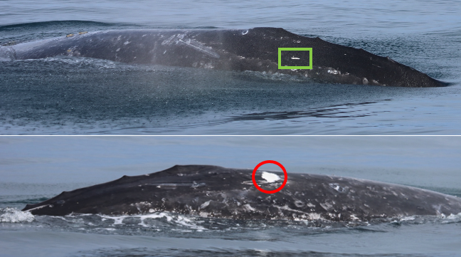


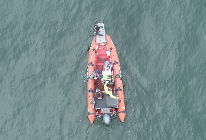
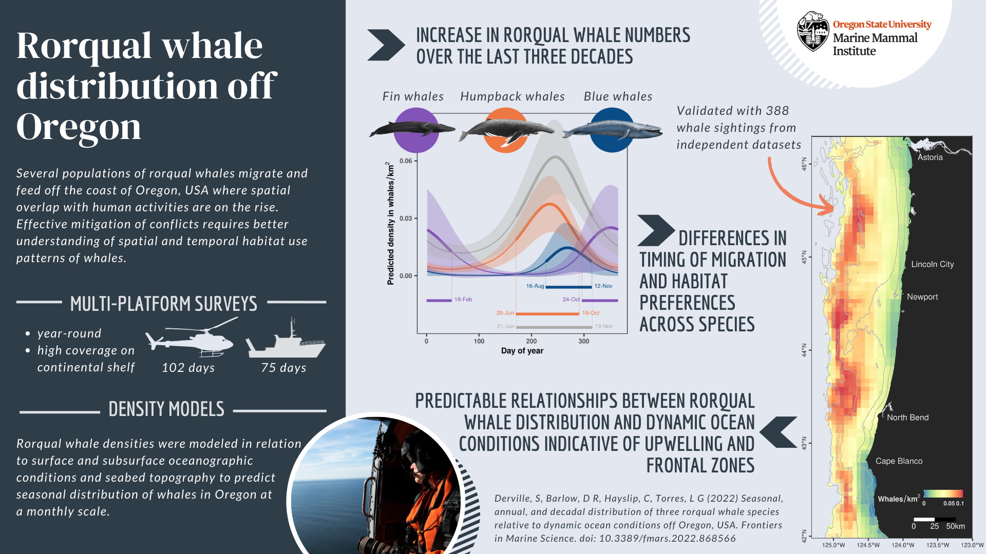
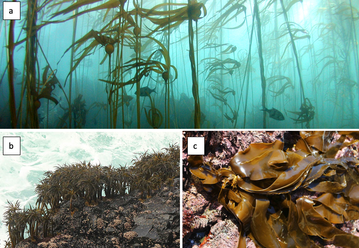


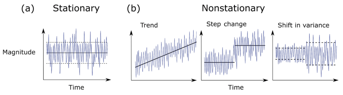
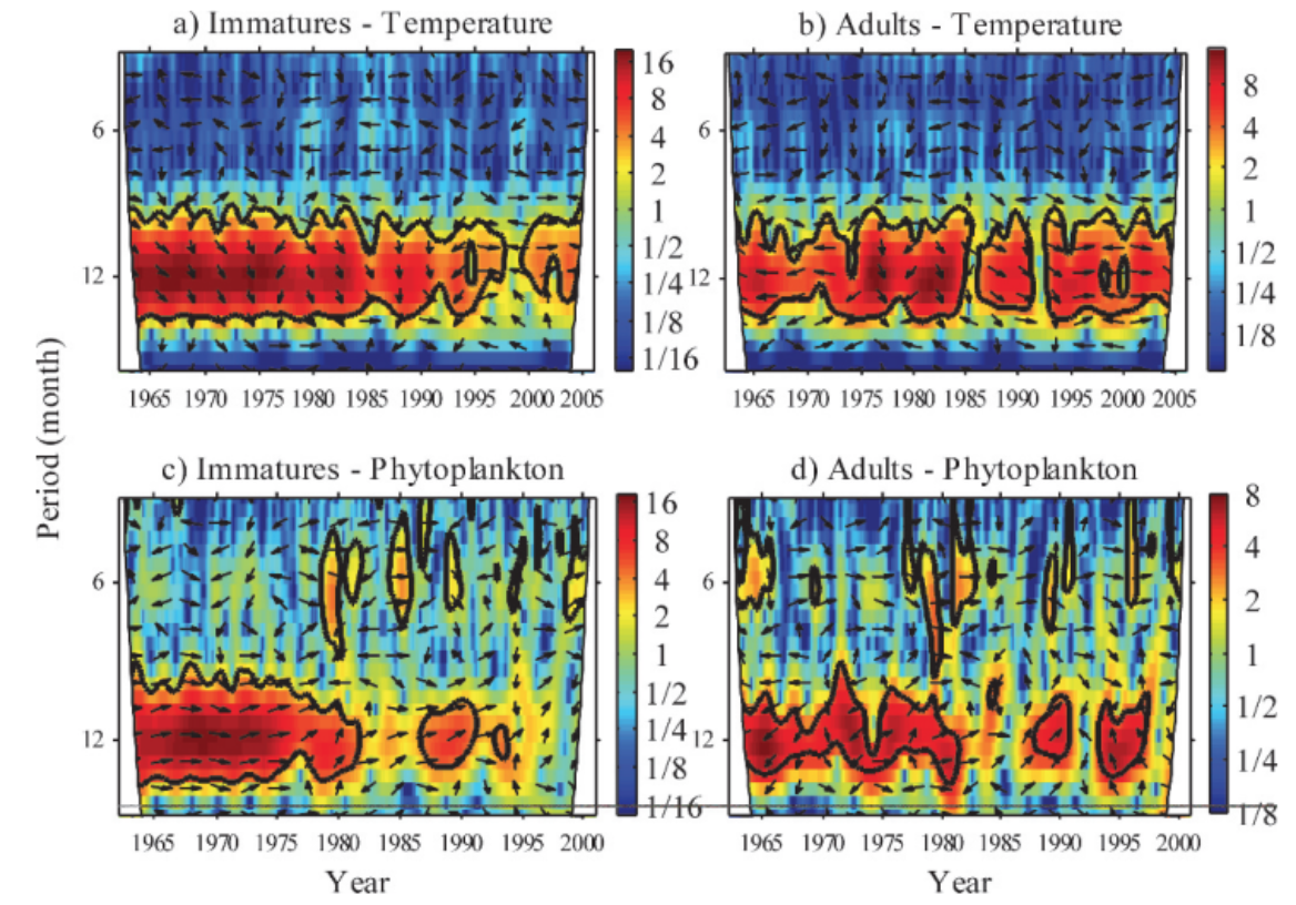

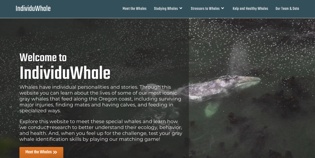

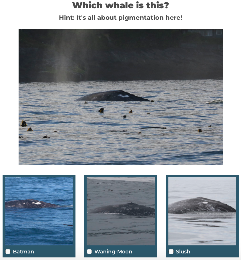
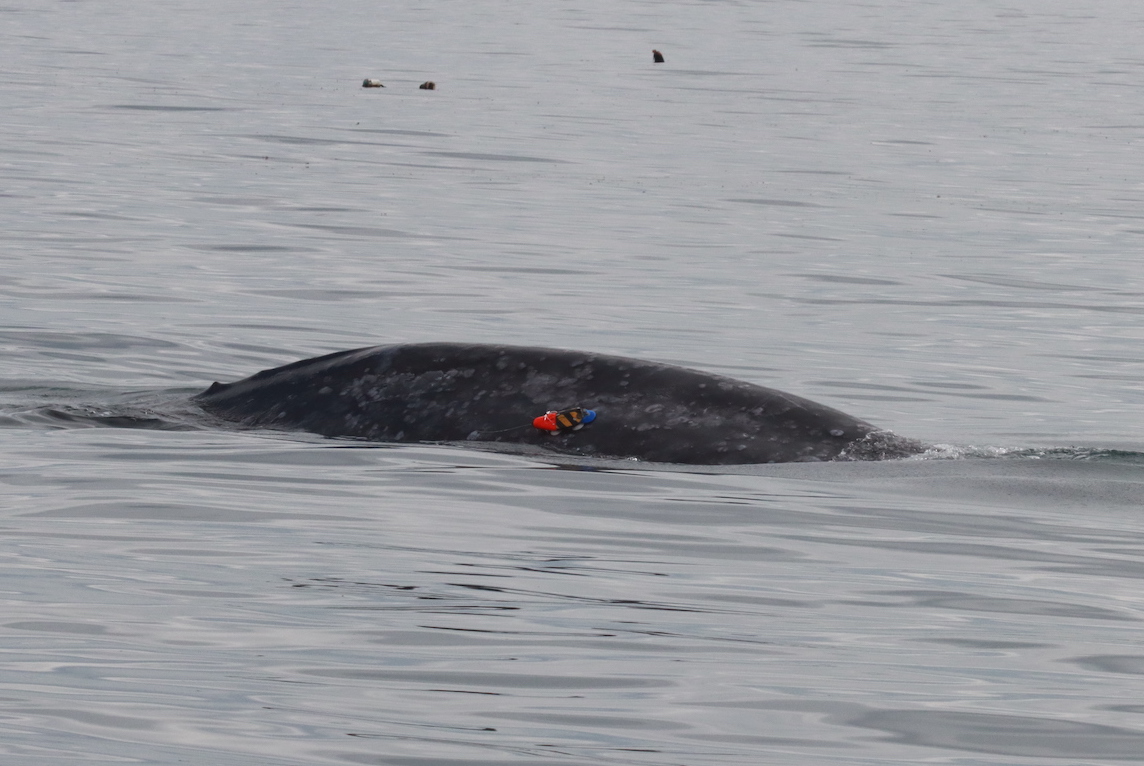


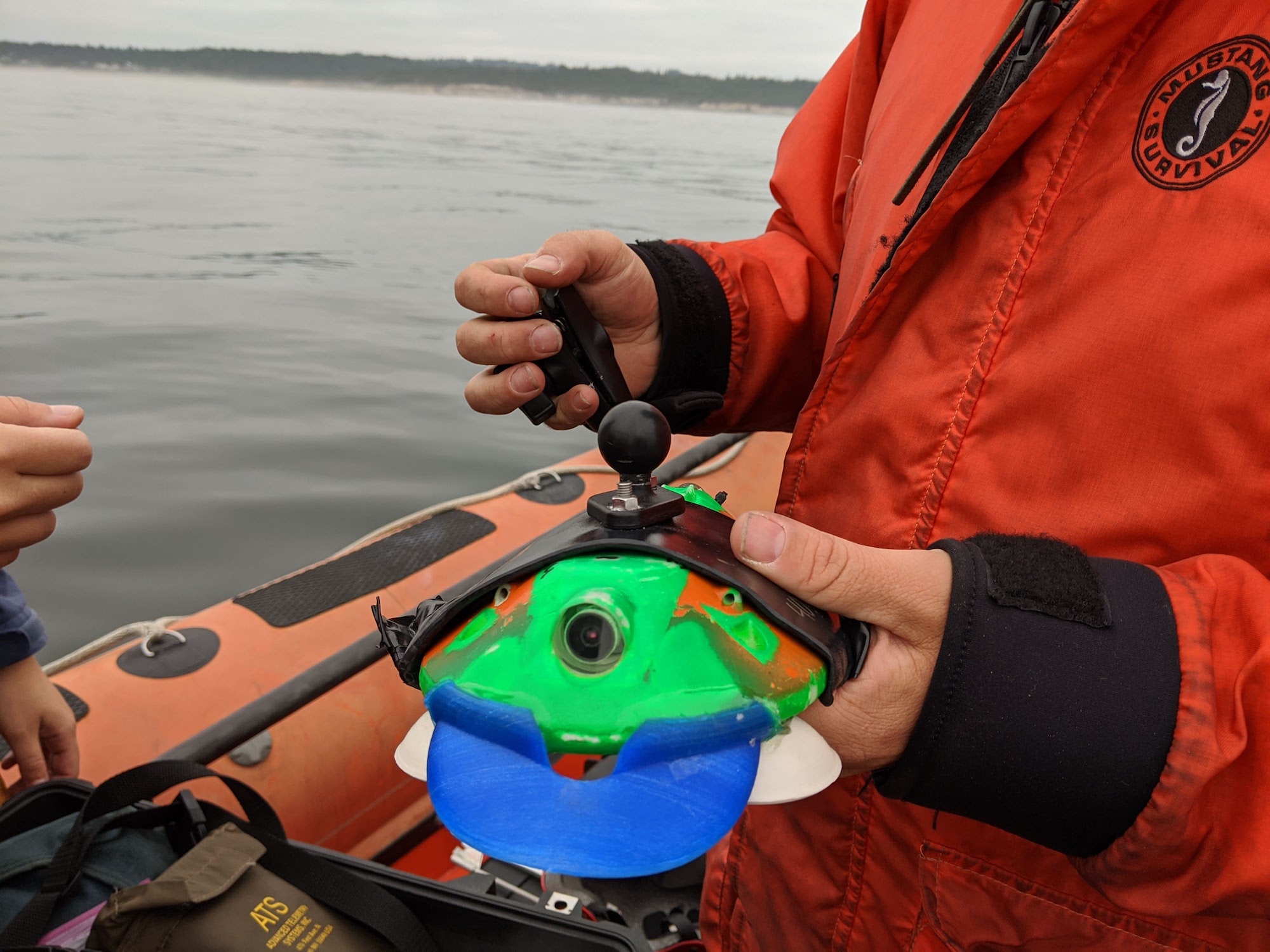


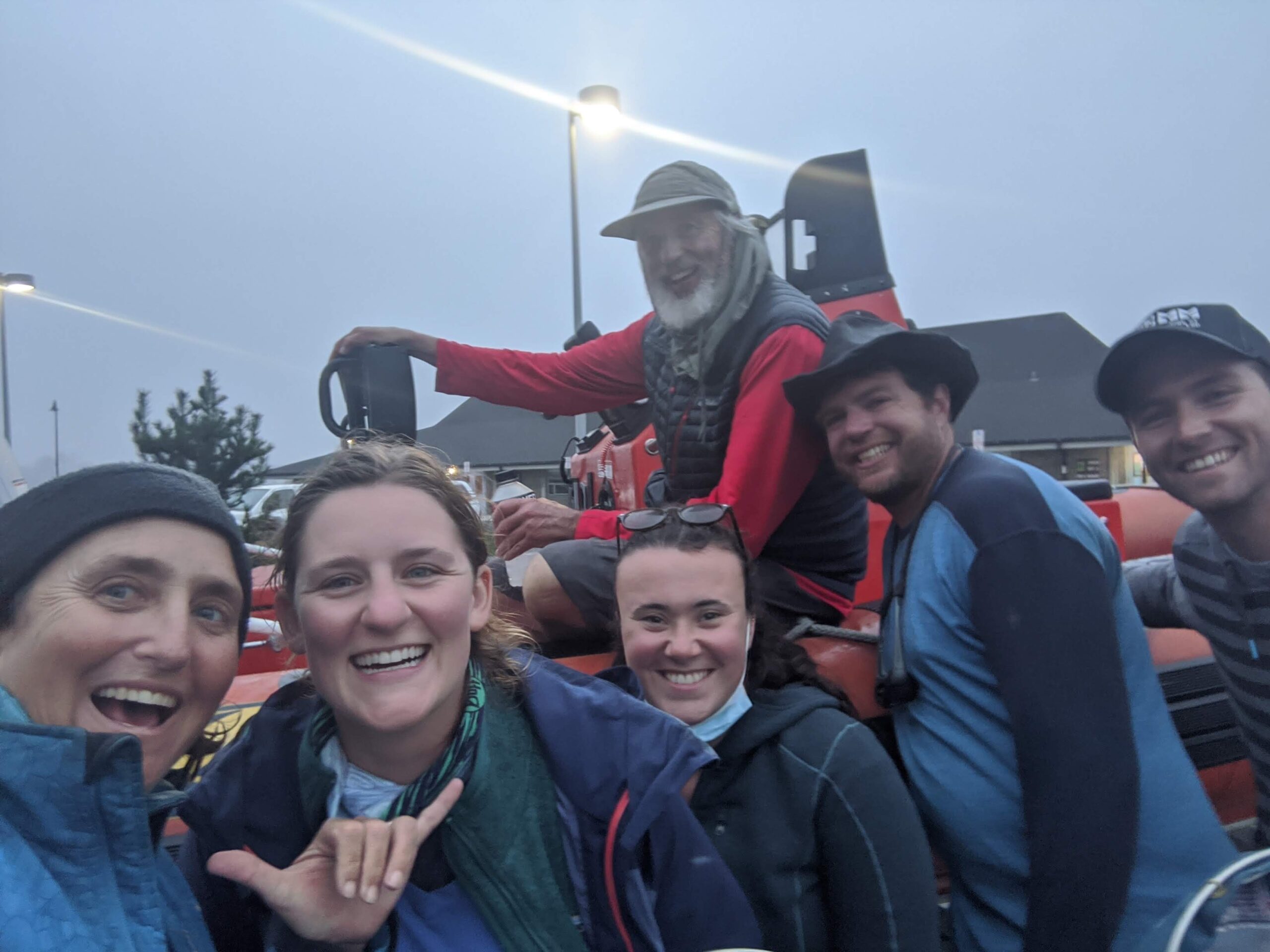


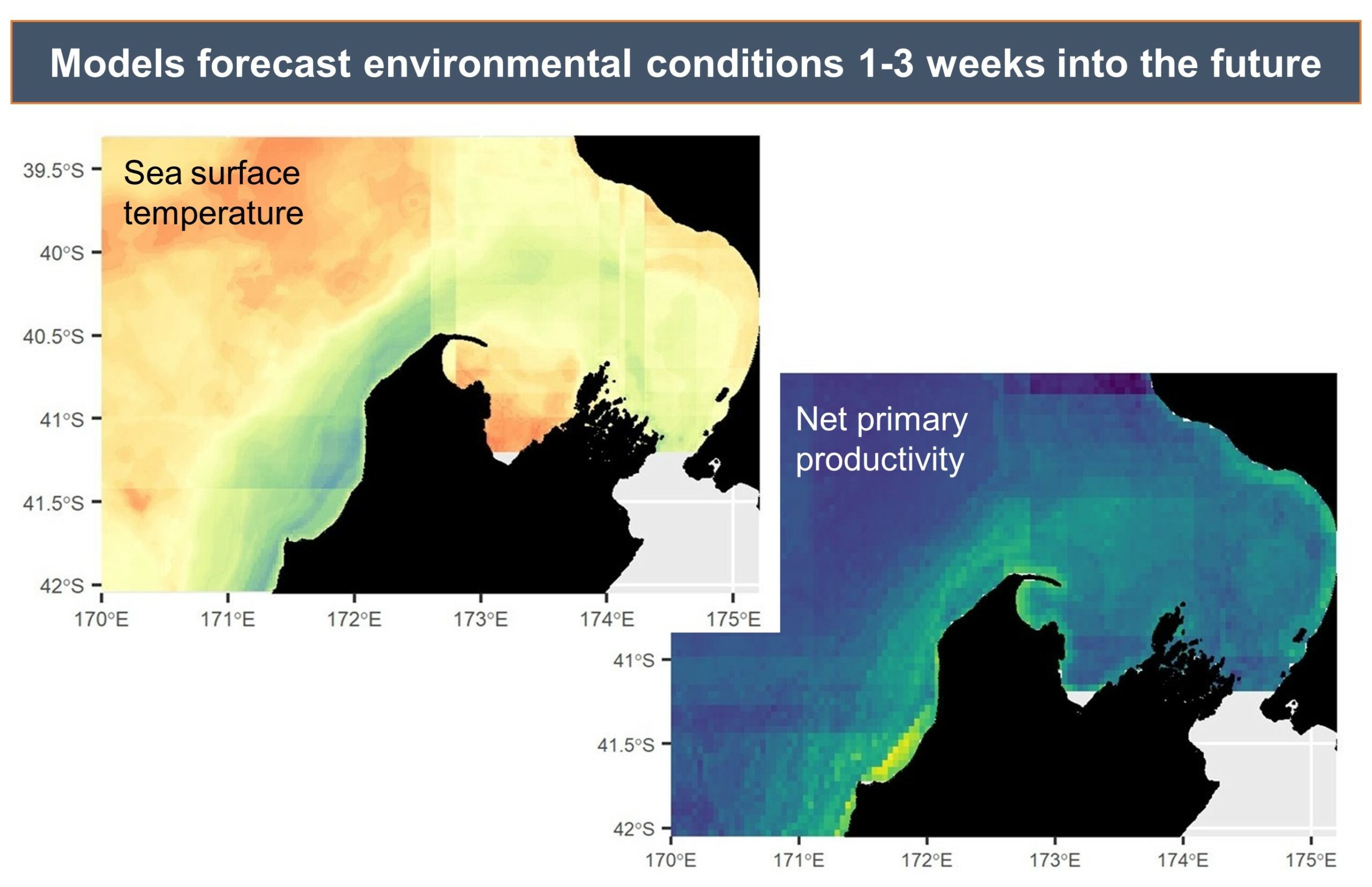

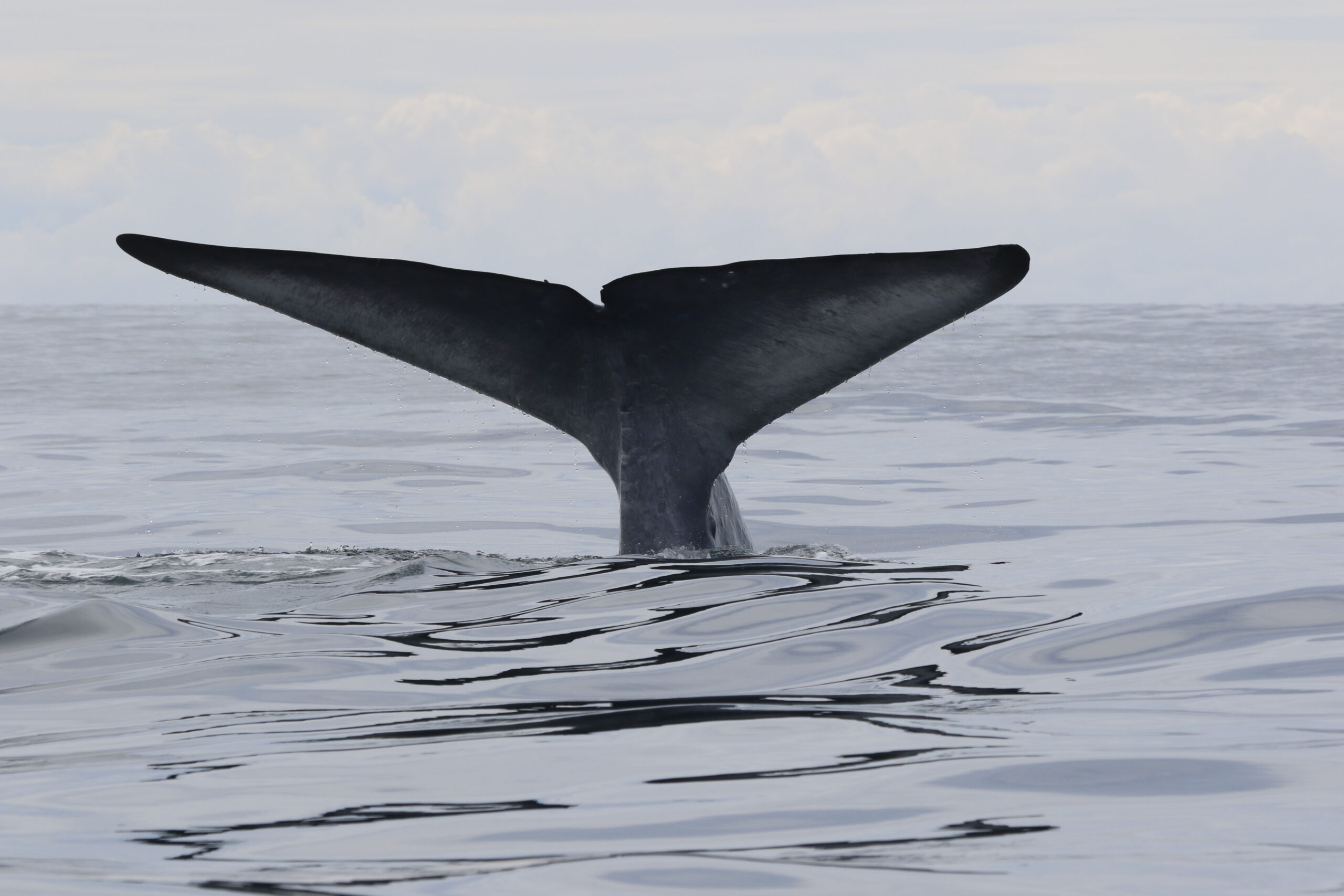
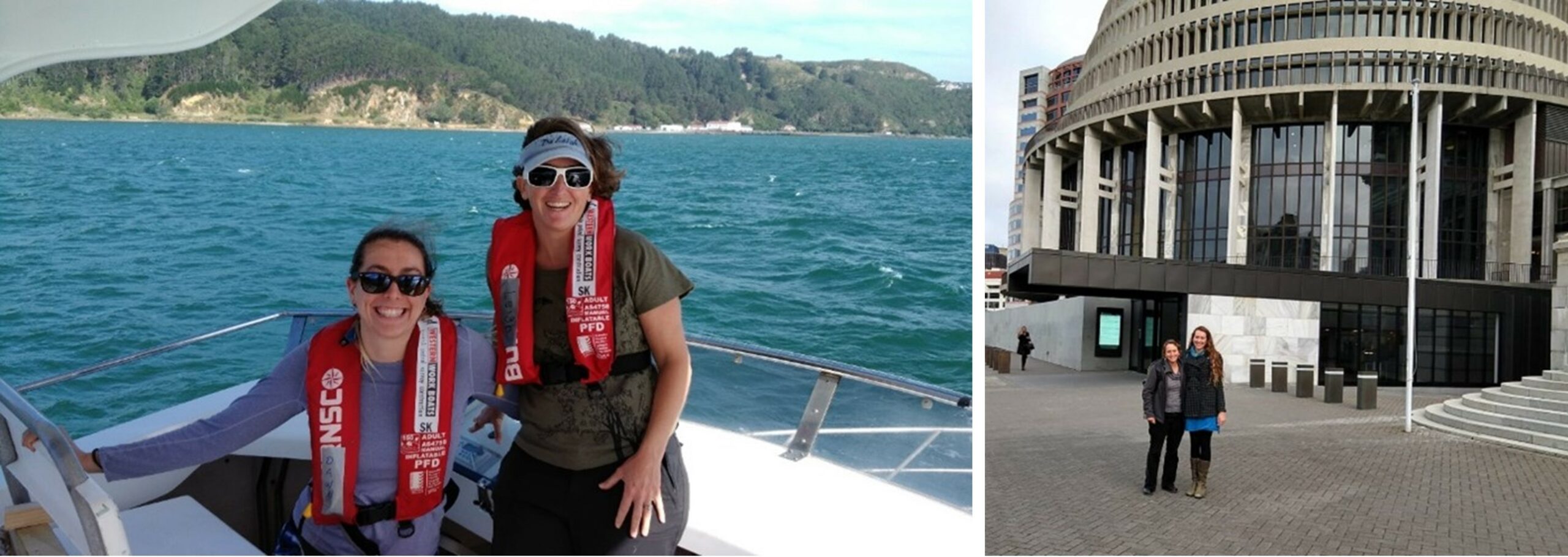

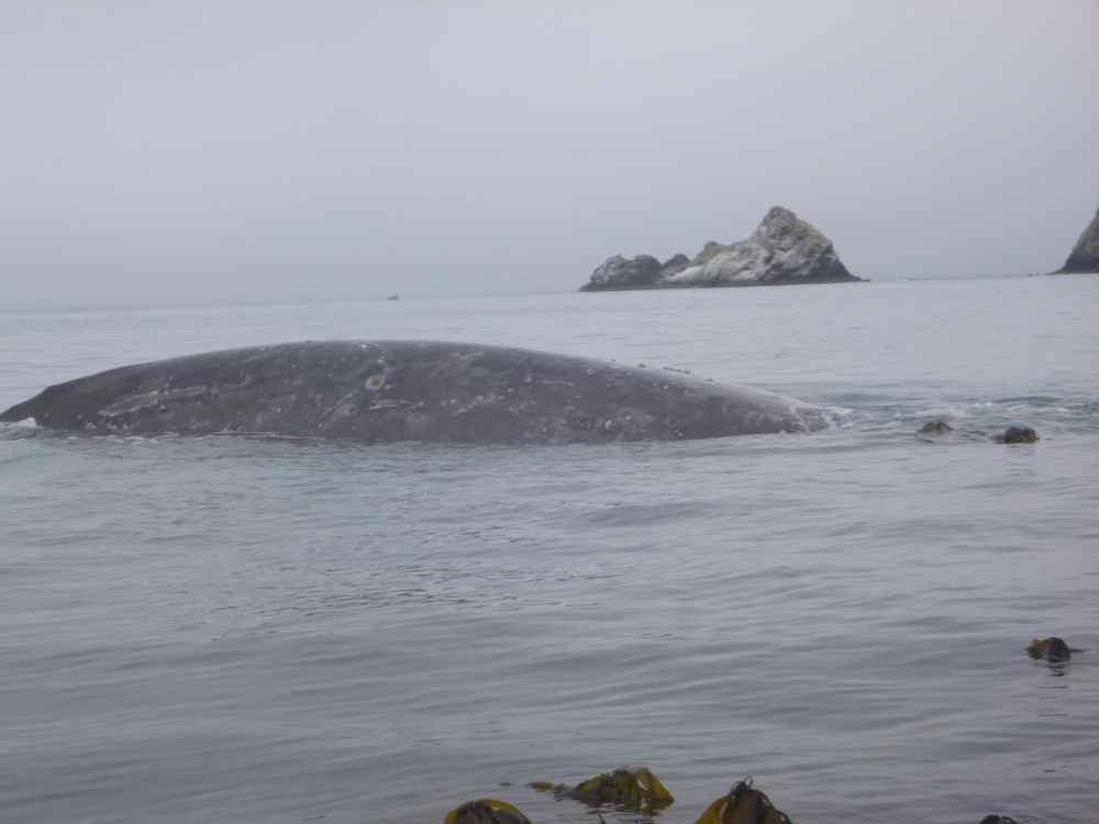


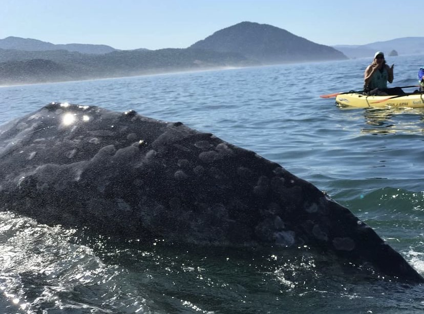


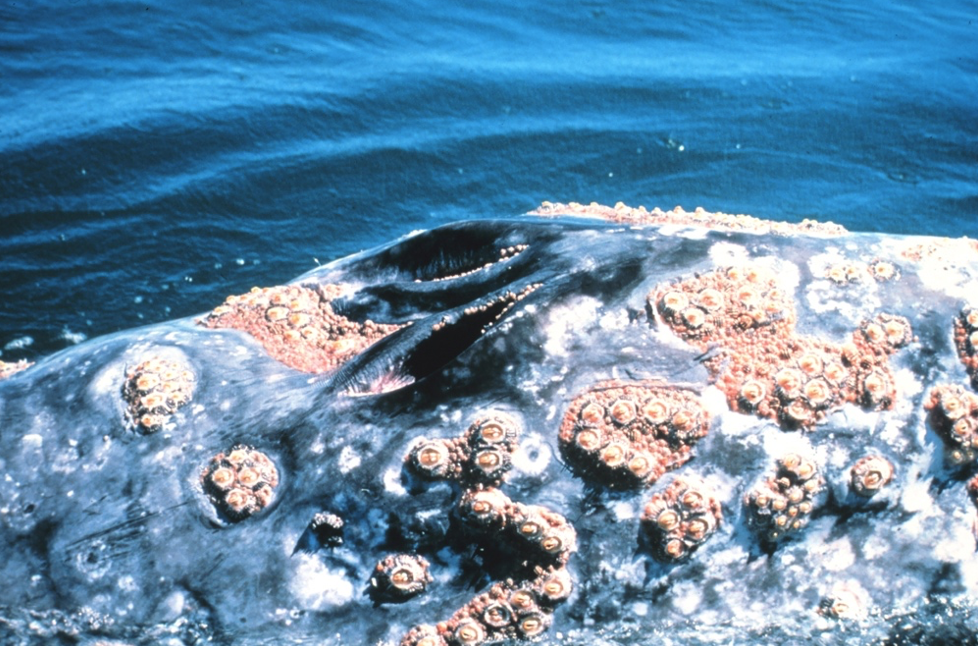