Do gray whales count calories? New GEMM Lab publication compares energetic values of prey available to gray whales on two feeding grounds in the eastern North Pacific

By Lisa Hildebrand, PhD student, OSU Department of Fisheries, Wildlife, & Conservation Sciences, Geospatial Ecology of Marine Megafauna Lab

Predators have high energetic requirements that must be met to ensure reproductive success and population viability. For baleen whales, this task is particularly challenging since their foraging seasons are typically limited to short temporal windows during summer months when they migrate to productive high latitude environments. Foraging success is a balancing act whereby baleen whales must maximize the amount of energy they intake, while minimizing the amount of energy they expend to obtain food. Maximization of energy intake can be achieved by targeting the most beneficial prey. How beneficial a particular prey type (or prey patch) is can depend on a number of factors such as abundance, density, quality, size, and availability. Determining why baleen whales target particular prey types or patches is an important factor to enhance our understanding of their ecology and can ultimately aid in informing their management and conservation.

The GEMM Lab has several research projects in Newport and Port Orford, Oregon, on the Pacific Coast Feeding Group (PCFG), which is a sub-group of gray whales from the Eastern North Pacific (ENP) population. While ENP gray whales feed in the Bering, Chukchi, and Beaufort Seas (Arctic) in the summer months, the PCFG utilizes the range from northern California, USA to northern British Columbia, Canada. Our work to date has revealed a number of new findings about the PCFG including that they successfully gain weight during the summer on Oregon foraging grounds (Soledade Lemos et al. 2020). Furthermore, females that consistently use the PCFG range as their foraging grounds have successfully reproduced and given birth to calves (Calambokidis & Perez 2017). Yet, the abundance of the PCFG (~250 individuals; Calambokidis et al. 2017) is two orders of magnitude smaller than the ENP population (~20,000; Stewart & Weller 2021). So, why do more gray whales not use the PCFG range as their foraging grounds when it provides a shorter migration while also allowing whales to meet their high energetic requirements and ensure reproductive success? There are several hypotheses regarding this ecological mystery including that prey abundance, density, quality, and/or availability are higher in the Arctic than in the PCFG range, thus justifying the much larger number of gray whales that migrate further north for the summer feeding season. 

Figure 1. Locations of prey samples collected with a light trap (open circles) or opportunistic collections of surface swarms of crab larvae (black triangles) in Newport, along the Oregon coast in the Pacific Northwest coast of the United States.

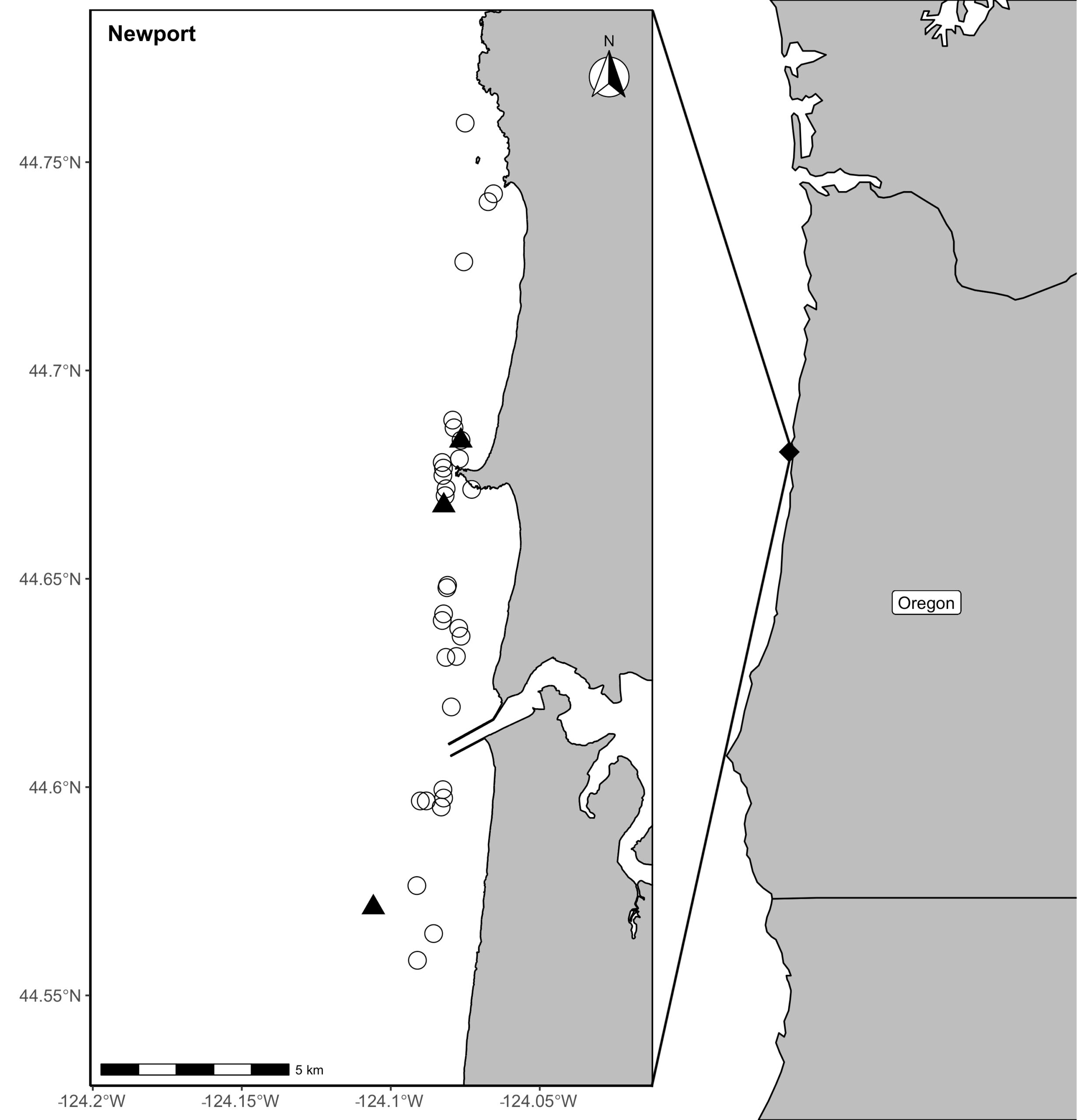
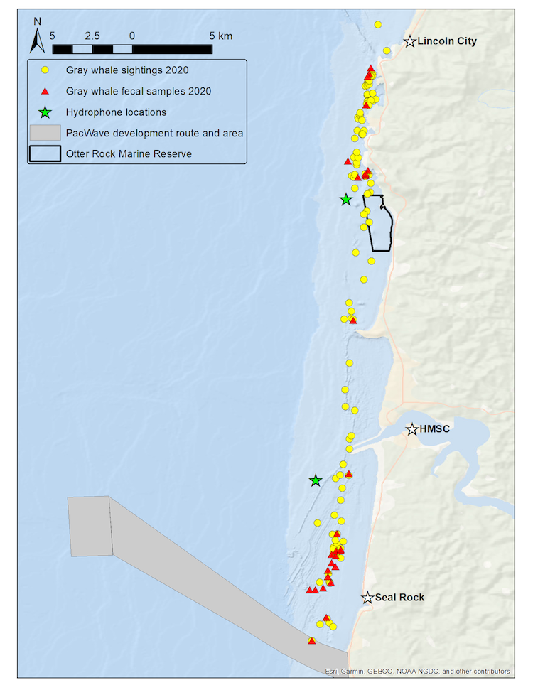
Our recent paper in Frontiers in Marine Science addressed the hypothesis that prey quality in the Arctic is higher than that of PCFG prey. To test this hypothesis, we first determined the quality (energetic value) of nearshore Oregon zooplankton species that PCFG gray whales are assumed to feed on (based on observations of fine-scale spatial and temporal overlap of foraging gray whales and sampled zooplankton). We obtained prey samples from nearshore reefs along the Oregon coast (Figure 1) as part of the GRANITE project using a light trap, which is a modified water jug with a weight and two floats attached to it, allowing the trap to sit approximately 1 meter above the seafloor. The trap contained a light which attracted zooplankton and effectively captured epibenthic prey of gray whales. Traps were left to soak overnight in locations where gray whales had been observed feeding extensively and collected the following morning. After identifying each specimen to species level and sorting them into reproductive stages, we used a bomb calorimeter to determine the caloric content of each species by month, year, and reproductive stage. We then compared these values to the literature-derived caloric value of the predominant benthic amphipod species that  ENP gray whales feed on in the Arctic. These comparisons allowed us to extrapolate the caloric values gained from each prey type to estimated energetic requirements of pregnant and lactating female gray whales (Villegas-Amtmann et al. 2017). 

Figure 2. Median caloric content and interquartile ranges by (A) species, (B) reproductive stage, and (C) month. Sizes of the zooplankton images are scaled at actual ratios relative to one another.

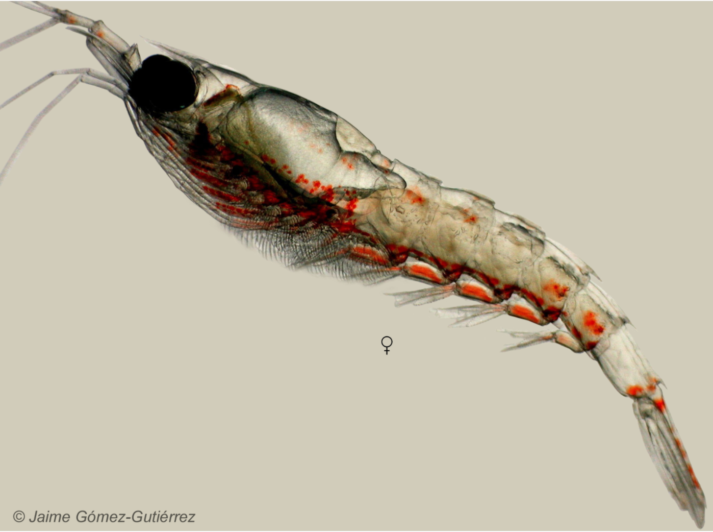
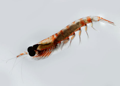
So, what did we find? Our sampling along the Oregon coast revealed six predominant zooplankton species: two mysid shrimp (Neomysis rayiiHolmesimysis sculpta), two amphipods (Atylus tridensPolycheria osborni), and two types of crab larvae (Dungeness crab megalopae, porcelain crab larvae). These six Oregon prey species showed significant differences in their caloric values, with N. rayii and Dungeness crab megalopae having significantly higher calories per gram than the other prey species (Figure 2), though Dungeness crab megalopae stood out as the caloric gold mines for feeding gray whales in the PCFG range. Furthermore, month and reproductive stage also influenced  the caloric content of some prey species, with gravid (aka pregnant) female mysid shrimp significantly increasing in calories throughout the summer (Figure 3).

Figure 3. Caloric content of different reproductive stages as a function of day of year (DOY; ranging from June to October) for the mysids Holmesimysis sculpta and Neomysis rayii, and the amphipod Atylus tridens. A. tridens is only represented on one panel due to small sample size of this species for the empty brood pouch and gravid reproductive stages. Asterisks indicate significant regressions (p<0.05).

The comparison of our Oregon prey caloric values to the predominant Arctic amphipod (Ampelisca macrocephala) proved our hypothesis wrong:  Arctic amphipods do not have higher caloric value than Oregon prey, which would have help to explain why many more gray whales feed in the Arctic. We found that two Oregon prey species (N. rayii and Dungeness crab megalopae) have higher caloric values than A. macrocephala. If we translate the caloric contents of these prey to gray whale energetic needs, these differences mean that lactating and pregnant gray whales feeding in the PCFG area would need between 0.7-1.03 and 0.22-0.33 metric tons of prey less per day if they fed on Dungeness crab megalopae or N. rayii, respectively, than a whale feeding on Arctic A. macrocephala (Figure 4). 

Figure 4. Daily prey requirements (A: metric tons; B: number of individuals) needed by pregnant and lactating female gray whales to meet their energetic requirements on the foraging ground. Energetic requirement estimates obtained from Villegas-Amtmann et al. (2017). Note the logarithmic scale of y-axis in panel (B).

If quality were the only prey metric that gray whales used to evaluate which food to eat, then it would make very little sense for so many gray whales to migrate to the Arctic when there are prey types of equal and greater quality available to them in the PCFG range. However, quality is not the only metric that influences gray whale foraging decisions. We therefore posit that the abundance, density, and availability of benthic amphipods in the Arctic are higher than the prey species found in the PCFG range. In fact, knowledge of the pulsed reproductive cycle of Dungeness and porcelain crabs allows us to conclude that the larvae of these two species are only available for a few weeks in the late spring and early summer on the Oregon coast. While mysid shrimp, such as N. rayii, are continuously available in the PCFG range throughout the summer, they may occur in less dense and more patchy aggregations than Arctic benthic amphipods. However, current estimates of prey density and abundance for either region are not available, and we do not have data on the energetic costs of the different foraging strategies. While there are still several unknowns, we have documented that higher prey quality in the Arctic is not the reason for the difference in gray whale foraging ground use in the eastern North Pacific.

References

Calambokidis, J., & Perez, A. 2017. Sightings and follow-up of mothers and calves in the PCFG and implications for internal recruitment. IWC Report SC/A17/GW/04 for the Workshop on the Status of North Pacific Gray Whales (La Jolla: IWC).

Calambokidis, J., Laake, J., & Perez, A. 2017. Updated analysis of abundance and population structure of seasonal gray whales in the Pacific Northwest, 1996-2015. IWC Report SC/A17/GW/05 for the Workshop on the Status of North Pacific Gray Whales (La Jolla: IWC).

Soledade Lemos, L., Burnett, J. D., Chandler, T. E., Sumich, J. L., & Torres, L. G. 2020. Intra- and inter-annual variation in gray whale body condition on a foraging ground. Ecosphere 11(4):e03094.

Stewart, J. D., & Weller, D. W. 2021. Abundance of eastern North Pacific gray whales 2019/2020. Department of Commerce, NOAA Technical Memorandum NMFS-SWFSC-639. United States: NOAA. doi:10.25923/bmam-pe91.

Villegas-Amtmann, S., Schwarz, L. K., Gailey, G., Sychenko, O., & Costa, D. P. 2017. East or west: the energetic cost of being a gray whale and the consequence of losing energy to disturbance. Endangered Species Research 34:167-183.

Little whale, big whale, swimming in the water: A quick history on how aerial photogrammetry has revolutionized the ability to obtain non-invasive measurements of whales

Dr. KC Bierlich, Postdoctoral Scholar, OSU Department of Fisheries, Wildlife, & Conservation Sciences, Geospatial Ecology of Marine Megafauna Lab

The morphology and body size of an animal is one of the most fundamental factors for understanding a species ecology. For instance, fish body size and fin shape can influence its habitat use, foraging behavior, prey type, physiological performance, and predator avoidance strategies (Fig 1). Morphology and body size can thus reflect details of an individual’s current health, likelihood of survival, and potential reproductive success, which directly influences a species life history patterns, such as reproductive status, growth rate, and energetic requirements. Collecting accurate morphological measurements of individuals is often essential for monitoring populations, and recent studies have demonstrated how animal morphology has profound implications for conservation and management decisions, especially for populations inhabiting anthropogenically-altered environments (Miles 2020) (Fig. 1). For example, in a study on the critically endangered European eel, De Meyer et al. (2020) found that different skulls sizes were associated with different ecomorphs (a local variety of a species whose appearance is determined by its ecological environment), which predicted different diet types and resulted with some ecomorphs having a greater exposure to pollutants and toxins than others. However, obtaining manual measurements of wild animal populations can be logistically challenging, limited by accessibility, cost, danger, and animal disturbance. These challenges are especially true for large elusive animals, such as whales that are often in remote locations, spend little time at the surface of the water, and their large size can preclude safe capture and live handling.

Figure 1. Top) A pathway framework depicting how the morphology of an animal influences its habitat use, behavior, foraging, physiology, and performance. These traits all affect how successful an animal is in its environment and can reflect an individual’s current health, likelihood of survival, and potential reproductive success. This individual success can then be scaled up to assess overall population health, which in turn can have direct implications for conservation. Bottom) an example of morphological differences in fish body size and fin shape from Walker et al. (2013). Fineness ratio (f) = length of body ­÷ max body width. 

Photogrammetry is a non-invasive method for obtaining accurate morphological measurements of animals from photographs. The two main types of photogrammetry methods used in wildlife biology are 1) single camera photogrammetry, where a known scale factor is applied to a single image to measure 2D distances and angles and 2) stereo-photogrammetry, where two or more images (from a single or multiple cameras) are used to recreate 3D models. These techniques have been used on domestic animals to measure body condition and estimate weight of dairy cows and lactating Mediterranean buffaloes (Negretti et al., 2008; Gaudioso et al., 2014) and on wild animals to measure sexual dimorphism in Western gorillas (Breuer et al., 2007), shoulder heights of elephants (Schrader et al., 2006), nutritional status of Japanese macaques (Kurita et al., 2012), and the body condition of brown bears (Shirane et al., 2020). Over 70 years ago, Leedy (1948) encouraged wildlife biologists to use aerial photogrammetry from aircraft for censusing wild animal populations and their habitats, where photographs can be collected at nadir (straight down) or an oblique angle, and the scale can be calculated by dividing the focal length of the camera by the altitude or by using a ratio of selected points in an image of a known size. Indeed, aerial photogrammetry has been wildly adopted by wildlife biologists and has proven useful in obtaining measurements in large vertebrates, such as elephants and whales.

Whitehead & Payne (1978) first demonstrated the utility of using aerial photogrammetry from airplanes and helicopters as a non-invasive technique for estimating the body length of southern right whales. Prior to this technique, measurements of whales were traditionally limited to assessing carcasses collected from scientific whaling operations, or opportunistically from commercial whaling, subsistence hunting, stranding events, and bycatch. Importantly, aerial photogrammetry provides a method to collect measurements of whales without killing them. This approach has been widely adopted to obtain body length measurements on a variety of whale and dolphin species, including bowhead whales (Cubbage & Calambokidis, 1987), southern right whales (Best & Rüther, 1992), fin whales (Ratnaswamy and Wynn, 1993), common dolphins (Perryman and Lynn, 1993), spinner dolphins (Perryman & Westlake 1998), and killer whales (Fearnbach et al. 2012). Aerial photogrammetry has also been used to measure body widths to estimate nutritive condition related to reproduction in gray whales (Perryman and Lynn, 2002) and northern and southern right whales (Miller et al., 2012). However, these studies collected photographs from airplanes and helicopters, which can be costly, limited by weather and infrastructure to support aircraft research efforts and, importantly, presents a potential risk to wildlife biologists (Sasse 2003). 

The recent advancement and commercialization of unoccupied aircraft systems (UAS, or drones) has revolutionized the ability to obtain morphological measurements from high resolution aerial photogrammetry across a variety of ecosystems (Fig. 2). Drones ultimately bring five transformative qualities to conservation science compared to airplanes and helicopters: affordability, immediacy, quality, efficiency, and safety of data collection. Durban et al. (2015) first demonstrated the utility of using drones for non-invasively obtaining morphological measurements of killer whales in remote environments. Since then, drone-based morphological measurements have been applied to a wide range of studies that have increased our understanding on different whale populations. For example, Leslie et al. (2020) used drone-based measurements of the skull to distinguish a unique sub-species of blue whales off the coast of Chile. Groskreutz et al. (2019) demonstrated how long-term nutritional stress has limited body growth in northern resident killer whales, while Stewart et al. (2021) found a decrease in body length of North Atlantic Right whales since 1981 that was associated with entanglements from fishing gear and may be a contributing factor to the decrease in reproductive success for this endangered population. 

Drone imagery is commonly used to estimate the body condition of baleen whales by measuring the body length and width of individuals. Recently, the GEMM Lab used body length and width measurements to quantify intra- and inter-seasonal changes in body condition across individual gray whales (Lemos et al., 2020). Drones have also been used to measure body condition loss in humpback whales during the breeding season (Christiansen et al., 2016) and to compare the healthy southern right whales to the skinnier, endangered North Atlantic right whales (Christiansen et al., 2020). Drone-based assessments of body condition have even been used to measure how calf growth rate is directly related to maternal loss during suckling (Christiansen et al., 2018), and even estimate body mass (Christiansen et al., 2019). 

Drone-based morphological measurements can also be combined with whale-borne inertial sensing tag data to study the functional morphology across several different baleen whale species. Kahane-Rapport et al. (2020) used drone measurements of tagged whales to analyze the biomechanics of how larger whales require longer times for filtering the water through their baleen when feeding. Gough et al. (2019) used size measurements from drones and swimming speeds from tags to determine that a whale’s “walking speed” is 2 meters per second – whether the largest of the whales, a blue whale, or the smallest of the baleen whales, an Antarctic minke whale. Size measurements and tag data were combined by Segre et al. (2019) to quantify the energetic costs of different sized whales when breaching. 

Taken together, drones have revolutionized our ability to obtain morphological measurements of whales, greatly increasing our capacity to better understand how these animals function and perform in their environments. These advancements in marine science are particularly important as these methods provide greater opportunity to monitor the health of populations, especially as they face increased threats from anthropogenic stressors (such as vessel traffic, ocean noise, pollution, fishing entanglement, etc.) and climate change. 

Drone-based photogrammetry is one of the main focuses of the GEMM Lab’s project on Gray whale Response to Ambient Noise Informed by Technology and Ecology (GRANITE). This summer we have been collecting drone videos to measure the body condition of gray whales feeding off the coast of Newport, Oregon (Fig. 2). As we try to understand the physiological stress response of gray whales to noise and other potential stressors, we have to account for the impacts of overall nutritional state of each individual whale’s physiology, which we infer from these body condition estimates. 

Figure 2. Drones can help collect images of whales to obtain morphological measurements using photogrammetry and help us fill knowledge gaps for how these animals interact in their environment and to assess their current health. Bottom photo is an image collected by the GEMM Lab of a gray whale being measured in MorphoMetriX software to estimate its body condition. 

References

Best, P. B., & Rüther, H. (1992). Aerial photogrammetry of southern right whales, Eubalaena australis. Journal of Zoology228(4), 595-614.

Breuer, T., Robbins, M. M., & Boesch, C. (2007). Using photogrammetry and color scoring to assess sexual dimorphism in wild western gorillas (Gorilla gorilla). American Journal of Physical Anthropology134(3), 369–382. https://doi.org/10.1002/ajpa.20678 

Christiansen, F., Vivier, F., Charlton, C., Ward, R., Amerson, A., Burnell, S., & Bejder, L. (2018). Maternal body size and condition determine calf growth rates in southern right whales. Marine Ecology Progress Series592, 267–281. 

Christiansen, F. (2020). A population comparison of right whale body condition reveals poor state of North Atlantic right whale, 1–43. 

Christiansen, F., Dujon, A. M., Sprogis, K. R., Arnould, J. P. Y., & Bejder, L. (2016). Noninvasive unmanned aerial vehicle provides estimates of the energetic cost of reproduction in humpback whales. Ecosphere7(10), e01468–18. 

Christiansen, F., Sironi, M., Moore, M. J., Di Martino, M., Ricciardi, M., Warick, H. A., … Uhart, M. M. (2019). Estimating body mass of free-living whales using aerial photogrammetry and 3D volumetrics. Methods in Ecology and Evolution10(12), 2034–2044. 

Cubbage, J. C., & Calambokidis, J. (1987). Size-class segregation of bowhead whales discerned through aerial stereo-photogrammetry. Marine Mammal Science3(2), 179–185. 

De Meyer, J., Verhelst, P., & Adriaens, D. (2020). Saving the European Eel: How Morphological Research Can Help in Effective Conservation Management. Integrative and Comparative Biology23, 347–349. 

Gaudioso, V., Sanz-Ablanedo, E., Lomillos, J. M., Alonso, M. E., Javares-Morillo, L., & Rodr\’\iguez, P. (2014). “Photozoometer”: A new photogrammetric system for obtaining morphometric measurements of elusive animals, 1–10.

Gough, W. T., Segre, P. S., Bierlich, K. C., Cade, D. E., Potvin, J., Fish, F. E., … Goldbogen, J. A. (2019). Scaling of swimming performance in baleen whales. Journal of Experimental Biology222(20), jeb204172–11. 

Groskreutz, M. J., Durban, J. W., Fearnbach, H., Barrett-Lennard, L. G., Towers, J. R., & Ford, J. K. B. (2019). Decadal changes in adult size of salmon-eating killer whales in the eastern North Pacific. Endangered Species Research40, 1 

Kahane-Rapport, S. R., Savoca, M. S., Cade, D. E., Segre, P. S., Bierlich, K. C., Calambokidis, J., … Goldbogen, J. A. (2020). Lunge filter feeding biomechanics constrain rorqual foraging ecology across scale. Journal of Experimental Biology223(20), jeb224196–8. 

Leedy, D. L. (1948). Aerial Photographs, Their Interpretation and Suggested Uses in Wildlife Management. The Journal of Wildlife Management12(2), 191. 

Lemos, L. S., Burnett, J. D., Chandler, T. E., Sumich, J. L., and Torres, L. G. (2020). Intra- and inter-annual variation in gray whale body condition on a foraging ground. Ecosphere 11.

Leslie, M. S., Perkins-Taylor, C. M., Durban, J. W., Moore, M. J., Miller, C. A., Chanarat, P., … Apprill, A. (2020). Body size data collected non-invasively from drone images indicate a morphologically distinct Chilean blue whale (Balaenoptera musculus) taxon. Endangered Species Research43, 291–304. 

Miles, D. B. (2020). Can Morphology Predict the Conservation Status of Iguanian Lizards? Integrative and Comparative Biology

Miller, C. A., Best, P. B., Perryman, W. L., Baumgartner, M. F., & Moore, M. J. (2012). Body shape changes associated with reproductive status, nutritive condition and growth in right whales Eubalaena glacialis and E. australis. Marine Ecology Progress Series459, 135–156. 

Negretti, P., Bianconi, G., Bartocci, S., Terramoccia, S., & Verna, M. (2008). Determination of live weight and body condition score in lactating Mediterranean buffalo by Visual Image Analysis. Livestock Science113(1), 1–7. https://doi.org/10.1016/j.livsci.2007.05.018 

Ratnaswamy, M. J., & Winn, H. E. (1993). Photogrammetric Estimates of Allometry and Calf Production in Fin Whales, \emph{Balaenoptera physalus}. American Society of Mammalogists74, 323–330. 

Perryman, W. L., & Lynn, M. S. (1993). Idendification of geographic forms of common dolphin(\emph{Delphinus Delphis}) from aerial photogrammetry. Marine Mammal Science9(2), 119–137. 

Perryman, W. L., & Lynn, M. S. (2002). Evaluation of nutritive condition and reproductive status of migrating gray whales (\emph{Eschrichtius robustus}) based on analysisof photogrammetric data. Journal Cetacean Research and Management4(2), 155–164. 

Perryman, W. L., & Westlake, R. L. (1998). A new geographic form of the spinner dolphin, stenella longirostris, detected with aerial photogrammetry. Marine Mammal Science14(1), 38–50. 

Sasse, B. (2003). Job-Related Mortality of Wildlife Workers in the United States, 1937- 2000, 1015–1020. 

Segre, P. S., Potvin, J., Cade, D. E., Calambokidis, J., Di Clemente, J., Fish, F. E., … & Goldbogen, J. A. (2020). Energetic and physical limitations on the breaching performance of large whales. Elife9, e51760.

Shirane, Y., Mori, F., Yamanaka, M., Nakanishi, M., Ishinazaka, T., Mano, T., … Shimozuru, M. (2020). Development of a noninvasive photograph-based method for the evaluation of body condition in free-ranging brown bears. PeerJ8, e9982. https://doi.org/10.7717/peerj.9982 

Shrader, A. M., M, F. S., & Van Aarde, R. J. (2006). Digital photogrammetry and laser rangefinder techniques to measure African elephants, 1–7. 

Stewart, J. D., Durban, J. W., Knowlton, A. R., Lynn, M. S., Fearnbach, H., Barbaro, J., … & Moore, M. J. (2021). Decreasing body lengths in North Atlantic right whales. Current Biology.

Walker, J. A., Alfaro, M. E., Noble, M. M., & Fulton, C. J. (2013). Body fineness ratio as a predictor of maximum prolonged-swimming speed in coral reef fishes. PloS one8(10), e75422.

Rorquals of the California Current

By Solène Derville, Postdoc, OSU Department of Fisheries, Wildlife, and Conservation Science, Geospatial Ecology of Marine Megafauna Lab

About 10 months have passed since I started working on OPAL, a project that aims to identify the co-occurrence between whales and fishing effort in Oregon to reduce entanglement risk. During this period, you would be surprised to know how little ecology I have actually done and how much time has been devoted to data processing! I compiled several million GPS trackline positions, processed hundreds of marine mammal observations, wrote several thousand lines of R code, downloaded and extracted a couple Gb of environmental data… before finally reaching the modeling phase of the OPAL project. And with it, finally comes the time to look more closely at the ecology and behavior of my species of interest. While the previous steps of the project were pretty much devoid of ecological reasoning, the literature homework now comes in handy to guide my choices regarding habitat use models, such as  selecting environmental predictors of whale occurrence, deciding on what seasons should be modeled, and choosing the spatio-temporal scale at which the data should be aggregated.

Whale diversity on the US west coast

The productive waters off the US west coast host a great diversity of cetaceans. Eight species of baleen whales are reported to occur there by NOAA fisheries: blue whales, Bryde’s whales, fin whales, gray whales, humpback whales, minke whales, North Pacific right whales and sei whales. Among them, no less than five are listed as Endangered under the Endangered Species Act. Whether they are only passing by or spending months feeding in the region, the timing and location where these animals are observed varies greatly by species and by population.

During the 113 hours of aerial survey effort and 264 hours of boat-based search conducted for the OPAL project, 563 groups of baleen whales have been observed to-date (up to mid-May 2021 to be exact… more data coming soon!). Among the observations where animals could be identified to the species level, humpback whales are preponderant, as they represent about half of the whale groups observed (n = 293). Blue (n = 41) and gray whales (n = 46) come next, the latter being observed in more nearshore waters. Finally, a few fin whale groups were observed (n = 28). The other baleen whale species reported by NOAA in the US west coast species list were very rarely or not observed at all during OPAL surveys.

The OPAL aerial surveys conducted in partnership with the United States Coast Guard (USCG) were specifically designed to study whales occurring on the continental shelf along the coast of Oregon. Hence, most of this survey effort is located in waters from 800 m to 30 m deep, which may explain the relatively low number of gray whales detected. Indeed, gray whales observed in Oregon may either be migrating along the coast to and from their breeding grounds in Baja California, or be part of the small Pacific Coast Feeding Group that forage in Oregon nearshore and shallow waters during the summer. This group of whales is one the main GEMM lab’s research focus, being at the core of no less than three ongoing research projects: AMBER, GRANITE, and TOPAZ.

So today, let’s turn our eyes to the sea horizon and talk about some other members of the baleen whale community: rorquals. Conveniently, the three species of baleen whales (gray whales aside) most commonly observed during OPAL surveys are all part of the rorqual family, a.k.a Balaenopteridae: humpback whales, blue whales and fin whales (Figure 1). They are morphologically characterized by the pleated throat grooves that allow them to engulf large quantities of food and water, for instance when lunge-feeding. Known cases of hybridization between these three species demonstrate their close relatedness (Jefferson et al., 2021)⁠. They all have worldwide distributions and display unequally understood migratory behaviors, seasonally traveling between warm tropical breeding grounds and temperate-polar feeding grounds. They occur in great numbers in productive waters such as the upwelling system of the California Current.

The three accomplices

Figure 1: Aerial view of three rorquals species: a humpback whale (left), a fin whale (center), and a blue whale (right). Photo credit: Leigh Torres and Craig Hayslip. Photos taken off the Oregon coast under NOAA/NMFS permit during USCG helicopter flights conducted as part of the OPAL project

Humpback whales (Megaptera novaeangliae) are easily differentiated from other rorquals because of their long pectoral fins (up to one third of their body length!), which inspired their scientific name, Megaptera, « big-winged » (Figure 1). Individuals observed in Oregon mostly belong to a mix of two Distinct Population Segments (DPS): the threatened Mexico and endangered Central American DPS. Although humpback whales from different DPS do not show any morphological differences, they are genetically distinct because they have been mating separately in distinct breeding grounds for generations and generations. This genetic differentiation has great implications in terms of conservation since the Central American DPS is recovering at a lesser rate than the Mexican and is therefore subject to different management measures (recovery plan, monitoring plan, designated critical habitats). Humpback whales migrate and feed off the US west coast, with a peak in abundance in the mid to late summer. Compared to other rorquals that are found in the open ocean, humpback whales are mostly observed on the continental shelf (Becker et al., 2019)⁠. They are considered to have a relatively generalist diet, as they feed on a mix of krill (Euphausiids) and fishes (e.g. anchovy, sardines) and are capable of switching their feeding behavior depending on relative prey availability (Fleming, Clark, Calambokidis, & Barlow, 2016; Fossette et al., 2017)⁠.

Blue whales (Balaenoptera musculus) are the largest animals ever known (max length 33 m, Jefferson et al., 2008), and sadly the most at risk of global extinction among our three species of interest (listed as « endangered » in the IUCN red list). They have a distinctive mottled blue and light gray skin, a slender body and a broad U-shaped head (or as some say « like a gothic arch », Figure 1). Blue whales tend to be open ocean animals, but they regroup seasonally to feed in highly productive nearshore areas such as the Southern California Bight (Becker et al. 2019, Abrahms et al. 2019). Blue whales migrating or feeding along the US west coast belong to the Eastern North Pacific stock and are subject to great research and conservation efforts. Contrary to their other rorqual counterparts, blue whales are quite picky eaters, as they exclusively feed on krill. This difference in diet leads to resource partitioning facilitating rorqual coexistence in the California Current (Fossette et al., 2017)⁠. These differences in feeding strategies have important implications for designing predictive models of habitat use.

Fin whales (Balaenoptera physalus) are nicknamed « greyhounds of the sea » due to their exceptional swim speed (max 46 km/h). They are a little smaller than blue whales (max length 27 m, Jefferson, Webber, & Pitman, 2008)⁠ but share a similar sleek and streamlined shape. Their coloration is their most distinctive feature: the left lower jaw being mostly dark while the right is white. V-shaped light-gray « chevrons » color their back, behind the head (Figure 1). The California/Oregon/Washington is one of the three stocks recognized in the North Pacific (NOAA Fisheries, 2018)⁠. Within this region, there is genetic evidence for a geographic separation north and south of Point Conception, CA (Archer et al., 2013)⁠. Like other rorquals, they are migratory, but their seasonal distribution is relatively less well understood as they appear to spend a lot of time in open oceans. For instance, a meta-analysis for the North Pacific found little evidence for fin whales using distinct calving areas (Mizroch, Rice, Zwiefelhofer, Waite, & Perryman, 2009)⁠. In the California Current System, satellite tracking has provided great insights into their space-use patterns. In the Southern California Bight, fin whales show year-round residency and seasonal shifts in habitat use as they move further offshore and north during the spring/summer (Scales et al., 2017)⁠. The Northern California Current offshore waters appeared to be used during the summer months by the whales tagged in the Southern California Bight. Yet, fin whales are observed year-round in Oregon (NOAA Fisheries, 2018)⁠.

Towards predictive models of rorqual distribution

Enough observations have now been collected as part of the OPAL project to be able to model the habitat use of some of these rorqual species. Based on 12 topographic (i.e., depth, slope, distance to canyons) and physical variables (temperature, chlorophyll-a, water column stratification, etc.), I have made my first attempt at predicting seasonal distribution patterns of humpback whales and blue whales in Oregon. These models will be improved in the coming months, with more data pouring in and refined parametrizations, but they already bring insights into the shared habitat use patterns of these species, as well as their specificities.

Across multiple cross-validations of the species-specific models, sea surface temperature, sea surface height and depth were recurrently selected among the most important variables influencing both humpback and blue whale distributions. Predicted densities of blue whales were relatively higher at less than 40 fathoms compared to humpback whales, although both species’ hotspots were located outside this newly implemented seasonal fishing limit (Figure 2). Higher densities were generally predicted off Newport and Port Orford, and north of North Bend.

Figure 2: Predicted densities of humpback and blue whales during the month of September 2018, 2019, and 2020 in Oregon waters (OPAL project). Core areas of use (predicted densities in the top 25%) are represented, with darker shades of blue and orange showing higher predicted densities. Dashed lines represent the tracklines followed by USCG monthly aerial surveys. The black line represents the 40 fathom isobath. Grey boxes overlayed on predictions delineate the areas of extrapolation where environmental conditions are non-analogous to the conditions in which the models were trained. Disclaimer: these model outputs are preliminary and should be interpreted with caution.

Once our rorqual models are finalized, we will work with our partners at the Oregon Department of Fisheries and Wildlife to overlay predicted whale hotspots with areas of high crab pot densities. This overlap analysis will help us understand the times and places where co-occurrence of suitable whale habitat and fishing activities put whales at risk of entanglement.

References

Archer, F. I., Morin, P. A., Hancock-Hanser, B. L., Robertson, K. M., Leslie, M. S., Bérubé, M., … Taylor, B. L. (2013). Mitogenomic Phylogenetics of Fin Whales (Balaenoptera physalus spp.): Genetic Evidence for Revision of Subspecies. PLoS ONE, 8(5). https://doi.org/10.1371/journal.pone.0063396

Becker, E. A., Forney, K. A., Redfern, J. V, Barlow, J., Jacox, M. G., Roberts, J. J., & Palacios, D. M. (2019). Predicting cetacean abundance and distribution in a changing climate. Diversity and Distributions, 25(4), 626–643. https://doi.org/10.1111/ddi.12867

Fleming, A. H., Clark, C. T., Calambokidis, J., & Barlow, J. (2016). Humpback whale diets respond to variance in ocean climate and ecosystem conditions in the California Current. Global Change Biology, 22, 1214–1224. https://doi.org/10.1111/gcb.13171

Fossette, S., Abrahms, B., Hazen, E. L., Bograd, S. J., Zilliacus, K. M., Calambokidis, J., … Croll, D. A. (2017). Resource partitioning facilitates coexistence in sympatric cetaceans in the California Current. Ecology and Evolution, 7, 9085–9097. https://doi.org/10.1002/ece3.3409

Jefferson, T. A., Palacios, D. M., Clambokidis, J., Baker, S. C., Hayslip, C. E., Jones, P. A., … Schulman-Janiger, A. (2021). Sightings and Satellite Tracking of a Blue / Fin Whale Hybrid in its Wintering and Summering Ranges in the Eastern North Pacific. Advances in Oceanography & Marine Biology, 2(4), 1–9. https://doi.org/10.33552/AOMB.2021.02.000545

Jefferson, T. A., Webber, M. A., & Pitman, R. L. (2008). Marine Mammals of the World. A comprehensive guide to their identification. Elsevier, London, UK.

Mizroch, S. A., Rice, D. W., Zwiefelhofer, D., Waite, J., & Perryman, W. L. (2009). Distribution and movements of fin whales in the North Pacific Ocean. Mammal Review, 39(3), 193–227. https://doi.org/10.1111/j.1365-2907.2009.00147.x

NOAA Fisheries. (2018). Fin whale stock assessment report ( Balaenoptera physalus physalus ): California / Oregon / Washington Stock.

Scales, K. L., Schorr, G. S., Hazen, E. L., Bograd, S. J., Miller, P. I., Andrews, R. D., … Falcone, E. A. (2017). Should I stay or should I go? Modelling year-round habitat suitability and drivers of residency for fin whales in the California Current. Diversity and Distributions, 23(10), 1204–1215. https://doi.org/10.1111/ddi.12611

Rock-solid GRANITE: Scaling the disturbance response of individual whales up to population level impacts

By Lisa Hildebrand, PhD student, OSU Department of Fisheries & Wildlife, Geospatial Ecology of Marine Megafauna Lab

Since early May, much of the GEMM Lab has been consumed by the GRANITE project, which stands for Gray whale Response to Ambient Noise Informed by Technology and Ecology. Two weeks ago, PhD student Clara Bird discussed our field work preparations, and since May 20th we have conducted five successful days of field work (and one unsuccessful day due to fog). If you are now expecting a blog about the data we have collected so far and whales we encountered, I am sorry to disappoint you. Rather, I want to take a big step back and provide the context of the GRANITE project as a whole, explain why this project and data collection is so important, and discuss what it is that we hope to achieve with our ever-growing, multidisciplinary dataset and team.

We use the Pacific Coast Feeding Group (PCFG) of gray whales that forage off the Oregon coast as our study system to better understand the ecological and physiological response of baleen whales to multiple stressors. Our field methodology includes replicate physiological and ecological sampling of this accessible baleen whale population with synoptic measurement of multiple types of stressors. We collect fecal samples for hormone analysis, conduct drone overflights of whales to collect body condition and behavioral data, record the ambient soundscape through deployment of two hydrophones, and conduct whale photo-identification to link all data streams to each individual whale of known sex, estimated age, and reproductive status. We resample these data from multiple individuals within and between summer foraging seasons, while exposed to different potential stressors occurring at different intensities and temporal periods and durations. The hydrophones are strategically placed with one in a heavily boat-trafficked (and therefore noisy) area close to the Port of Newport, while the second is located in a relatively calm (and therefore quieter) spot near the Otter Rock Marine Reserve (Fig. 1). These hydrophones provide us with information about both natural (e.g. killer whales, wind, waves) and anthropogenic (e.g. boat traffic, seismic survey, marine construction associated with PacWave wave energy facility development) noise that may affect gray whales. During sightings with whales, we also drop GoPro cameras and sample for prey to better understand the habitats where whales forage and what they might be consuming.

Figure 1. Map of GRANITE study area from Seal Rock to Lincoln City with gray whale sightings (yellow circles) and and fecal samples collected (red triangles) from the 2020 field season. Green stars represent the two hydrophone locations. Source: L. Torres.

GEMM Lab PI Dr. Leigh Torres initiated this research project in 2015 and established partnerships with acoustician Dr. Joe Haxel and (then) PhD student Dr. Leila Lemos. Since then, the team working on this project has grown considerably to provide expertise in the various disciplines that the project integrates. Leigh is currently joined at the GRANITE helm by 4 co-PIs: Dr. Haxel, endocrinologist Dr. Kathleen Hunt, biological statistician Dr. Leslie New, and physiologist Dr. Loren Buck. Drs. Alejandro Fernandez Ajo, KC Bierlich and Enrico Pirotta are postdoctoral scholars who are working on the endocrinology, photogrammetry, and biostatistical modelling components, respectively. Finally, Clara and myself are partially funded through this project for our PhD research, with Clara focusing on the links between behavior, body condition, individualization, and habitat, while I am tackling questions about the recruitment and site fidelity of the PCFG (more about these topics below). 

Faculty Research Assistant Todd Chandler supervises PhD student Clara Bird during her maiden drone flight over a whale. Source: L. Torres.

The ultimate goal of this project is to use the PCFG as a case study to quantify baleen whale physiological response to different stressors and model the subsequent impacts on the population by implementing our long-term, replicate dataset into a framework called Population consequences of disturbance (PCoD; Fig. 2). PCoD is built upon the underlying concept that changes in behavior and/or physiology caused by disturbance (i.e. noise) affect the fitness of individuals by impacting their health and vital rates, such as survival, reproductive success, and growth rate (Pirotta et al. 2018). These impacts at the individual level may (or may not) affect the population as a whole, depending on what proportion of individuals in the population are affected by the disturbance and the intensity of the disturbance effect on each individual. The PCoD framework requires quantification of four stages: a) the physiological and/or behavioral changes that occur as a result of exposure to a stressor (i.e. noise), b) the acute effects of these physiological and/or behavioral responses on individual vital rates, and their chronic effects via individual health, c) the way in which changes in health may affect the vital rates of individuals, and d) how changes in individual vital rates may affect population dynamics (Fig. 2; Pirotta et al. 2018). While four stages may not sound like a lot, the amount and longevity of data needed to quantify each stage is immense. 

Figure 2. Conceptual framework of the population consequences of disturbance (PCoD). Letters (A-D) represent the four stages that require quantification in order for PCoD to be implemented. Each colored box represents external (ecological drivers, stressors) and internal (physiology, health, vital rates, behavior) factors that can change over time that are measured for each individual whale (dashed grey boundary line). The effects are then integrated across all individuals in the population to project their effects on the population’s dynamics. Figure and caption adapted from Pirotta et al. 2018.

The ability to detect a change in behavior or physiology often requires an understanding of what is “normal” for an individual, which we commonly refer to as a baseline. The best way to establish a baseline is to collect comprehensive data over a long time period. With our data collection efforts since 2015 of fecal samples, drone flights and photo identification, we have established useful baselines of behavioral and physiological data for PCFG gray whales. These baselines are particularly impressive since it is typically difficult to collect repeated measurements of hormones and body condition from the same individual baleen whale across multiple years. These repeated measurements are important because, like all mammals, hormones and body condition vary across life history phases (i.e., with pregnancy, injury, or age class) and across time (i.e., good or bad foraging conditions). To achieve these repeated measurements, GRANITE exploits the high degree of intra- and inter-annual site fidelity of the PCFG, their accessibility for study due to their affinity for nearshore habitat use, and the long-term sighting history of many whales that provides sex and approximate age information. Our work to-date has already established a few important baselines. We now know that the body condition of PCFG gray whales increases throughout a foraging season and can fluctuate considerably between years (Soledade Lemos et al. 2020). Furthermore, there are significant differences in body condition by reproductive state, with calves and pregnant females displaying higher body conditions (Soledade Lemos et al. 2020). Our dataset has also allowed us to validate and quantify fecal steroid and thyroid hormone metabolite concentrations, providing us with putative thresholds to identify a stressed vs. not stressed whale based on its hormone levels (Lemos et al. 2020).

PhD student Lisa Hildebrand and GRANITE co-PI Dr. Kathleen Hunt collecting a fecal sample. Source: L. Torres.

We continue to collect data to improve our understanding of baseline PCFG physiology and behavior, and to detect changes in their behavior and physiology due to disturbance events. All these data will be incorporated into a PCoD framework to scale from individual to population level understanding of impacts. However, more data is not the only thing we need to quantify each of the PCoD stages. The implementation of the PCoD framework also depends on understanding several aspects of the PCFG’s population dynamics. Specifically, we need to know whether recruitment to the PCFG population occurs internally (calves born from “PCFG mothers” return to the PCFG) or externally (immigrants from the larger Eastern North Pacific gray whale population joining the PCFG as adults). The degree of internal or external recruitment to the PCFG population should be included in the PCoD model as a parameter, as it will influence how much individual level disturbance effects impact the overall health and viability of the population. Furthermore, knowing residency times and home ranges of whales within the PCFG is essential to understand exposure durations to disturbance events. 

To assess both recruitment and residency patterns of the PCFG, I am undertaking a large photo-identification effort, which includes compiling sightings and photo data across many years, regions, and collaborators. Through this effort we aim to identify calves and their return rate to the population, the rate of new adult recruits to the population, and the spatial residency of individuals in our study system. Although photo-id is a basic, commonplace method in marine mammal science, its role is critical to tracking individuals over time to understand population dynamics (in a non-invasive manner, no less). A large portion of my PhD research will focus on the tedious yet rewarding task of photo-id data management and matching in order to address these pressing knowledge gaps on PCFG population dynamics needed to implement the PCoD model that is an ultimate goal of GRANITE. I am just beginning this journey and have already pinpointed many analytical and logistical hurdles that I need to overcome. I do not anticipate an easy path to addressing these questions, but I am extremely eager to dig into the data, reveal the patterns, and integrate the findings into our rock-solid GRANITE project.  

Funding for the GRANITE project comes from the Office of Naval Research, the Department of Energy, Oregon Sea Grant, the NOAA/NMFS Ocean Acoustics Program, and the OSU Marine Mammal Institute.

References

Lemos, L.S., Olsen, A., Smith, A., Chandler, T.E., Larson, S., Hunt, K., and L.G. Torres. 2020. Assessment of fecal steroid and thyroid hormone metabolites in eastern North Pacific gray whales. Conservation Physiology 8:coaa110.

Pirotta, E., Booth, C.G., Costa, D.P., Fleishman, E., Kraus, S.D., Lusseau, D., Moretti, D., New, L.F., Schick, R.S., Schwarz, L.K., Simmons, S.E., Thomas, L., Tyack, P.L., Weise, M.J., Wells, R.S., and J. Harwood. 2018. Understanding the population consequences of disturbance. Ecology and Evolution 8(19):9934-9946.

Soledade Lemos, L., Burnett, J.D., Chandler, T.E., Sumich, J.L., and L.G. Torres. 2020. Intra- and inter-annual variation in gray whale body condition on a foraging ground. Ecosphere 11(4):e03094.

Into the Krillscape: A Remote Expedition in Research and Mentorship

By Rachel Kaplan, PhD student, Oregon State University College of Earth, Ocean, and Atmospheric Sciences and Department of Fisheries and Wildlife, Geospatial Ecology of Marine Megafauna Lab

What are the most unexpected things you’ve done on Zoom in the last year? Since the pandemic dramatically changed all our lives in 2020, I think we’ve all been surprised by the diversity of things we’ve done remotely. I’ve baked bagels with a friend in Finland, done oceanography labs from my kitchen, had dance parties with people across the country, and conducted an award ceremony for my family’s Thanksgiving scavenger hunt – all on Zoom. Over the last several months, I’ve also mentored an Undergraduate Research, Scholarship, & the Arts (URSA) Engage student, named Amanda. Although we haven’t met in person yet, we’ve been connecting over Zoom since October. 

Amanda is an Ocean Sciences student working with me and Dr. Kim Bernard (CEOAS) to conduct a literature review about the two species of krill found off the coast of Oregon. Thysanoessa spinifera and Euphausia pacifica are an important food source for many of the animals that live off our coast — including blue, humpback, and fin whales. I am trying to learn how krill distributions shape those of humpback and blue whales as part of project OPAL, as well as which oceanographic factors drive krill abundances and distributions.

Thysanoessa spinifera (source: Scripps Institute of Oceanography). 

We’re also interested in T. spinifera and E. pacifica for the crucial roles they serve in ecosystems, beyond providing dinner for whales. Krill do many things that are beneficial to ecosystems and people, termed “ecosystem services.” These include facilitating carbon drawdown from the surface ocean to the deep, supporting lucrative fisheries species like salmon, flatfish, and rockfish, and feeding seabirds like auklets and shearwaters. We want to understand more fully the niche that T. spinifera and E. pacifica each fill off the coast of Oregon, which will help us anticipate how these important animals can be impacted by forces such as global climate change and marine management efforts.

Trying to understand the ecosystem services fulfilled by krill is inherently interdisciplinary, which means we have to learn a lot of new things, making this project a lot of fun. The questions Amanda and I have pursued together have ranged from intensely specific, to surprisingly broad. How many calories do blue whales need to eat in a day? How many krill do salmon need to eat? How big are krill fecal pellets, and how fast do they sink?

Trying to answer these questions has basically amounted to a heroic scouring of the internet’s krillscape by Amanda. She has hunted down papers dating back to the 1960s, pulled together findings from every corner of the world, and pursued what she refers to as “treasure troves” of data. In the process, she has also revealed the holes that exist in the literature, and given us new questions. This is the basis of the scientific process: understanding the current state of knowledge, identifying gaps in that knowledge, and developing the questions and methods needed to fill those gaps.

Euphausia pacifica (source: University of Irvine California, Peter J. Bryant).

Filling in knowledge gaps about T. spinifera and E. pacifica can help us better understand these animals, the ecosystems where they live, and the whales and other animals that depend on them for prey. It’s exciting to know that we will have the opportunity to help fill some of these gaps, as both Amanda and I continue this research over the course of our degrees.

Being able to engage in remote research and mentorship has been really rewarding, and it has shown me how far we’ve all come over the last year. Learning how to work together remotely has been crucial as we have adjusted to the funny new normal of the pandemic. As much as I miss working with people in person, I’ve learned that there’s a lot of great connection to be found even in remote collaboration – I’ve loved meeting Amanda’s pets on Zoom, learning about her career goals, and seeing her incredibly artistic representations of the carbon cycle held up to the camera.

Even though most of our conversations take place on Zoom from our homes, this research still feels plugged into a bigger community. Amanda and I also join Kim’s bigger Zooplankton Ecology Lab meetings, which include two other graduate students and eight undergraduate students, all of whom are working on zooplankton ecology questions that span from the Arctic to the Antarctic. Even though we’ve never met in person, a supportive and curious community has developed among all of us, which I know will persist when we can move back to in-person research and mentorship.

The right tool for the job: examining the links between animal behavior, morphology and habitat

Clara Bird, PhD Student, OSU Department of Fisheries and Wildlife, Geospatial Ecology of Marine Megafauna Lab

In order to understand a species’ distribution, spatial ecologists assess which habitat characteristics are most often associated with a species’ presence. Incorporating behavior data can improve this analysis by revealing the functional use of each habitat type, which can help scientists and managers assign relative value to different habitat types. For example, habitat used for foraging is often more important than habitat that a species just travels through. Further complexity is added when we consider that some species, such as gray whales, employ a variety of foraging tactics on a variety of prey types that are associated with different habitats. If individual foraging tactic specialization is present, different foraging habitats could be valuable to specific subgroups that use each tactic. Consequently, for a population that uses a variety of foraging tactics, it’s important to study the associations between tactics and habitat characteristics.

Lukoschek and McCormick’s (2001) study investigating the spatial distribution of a benthic fish species’ foraging behavior is a great example of combining data on behavior, habitat, and morphology.  They collected data on the diet composition of individual fish categorized into different size classes (small, medium, and large) and what foraging tactics were used in which reef zones and habitat types. The foraging tactics ranged from feeding in the water column to digging (at a range of depths) in the benthic substrate. The results showed that an interesting combination of fish behavior and morphology explained the observed diet composition and spatial distribution patterns. Small fish foraged in shallower water, on smaller prey, and primarily employed the water column and shallow digging tactics. In contrast, large fish foraged in deep water, on larger prey, and primarily fed by digging deeper into the seafloor (Figure 1). This pattern is explained by both morphology and behavior. Morphologically, the size of the feeding apparatus (mouth gape size) affects the size of the prey that a fish can feed on. The gape of the small fish is not large enough to eat the larger prey that large fish are able to consume. Behaviorally, predation risk also affects habitat selection and tactic use. Small fish are at higher risk of being predated on, so they remain in shallow areas where they are more protected from predators and they don’t dig as deep to forage because they need to be able to keep an eye out for predators. Interestingly, while they found a relationship between the morphology of the fish and habitat use, they did not find an association between specific feeding tactics and habitat types.

Figure 1. Figure from Lukoschek and McCormick (2001) showing that small fish (black bar) were found in shallow habitat while large fish (white bar) were found in deep habitat.

Conversely, Torres and Read (2009) did find associations between theforaging tactics of bottlenose dolphins in Florida Bay, FL and habitat type. Dolphins in this bay employ three foraging tactics: herd and chase, mud ring feeding, and deep diving. Observations of the foraging tactics were linked to habitat characteristics and individual dolphins. The study found that these tactics are spatially structured by depth (Figure 2), with deep diving occurring in deep water whereas mud ring feeding occurrs in shallower water. They also found evidence of individual specialization! Individuals that were observed deep diving were not observed mud ring feeding and vice-versa. Furthermore, they found that individuals were found in the habitat type associated with their preferred tactic regardless of whether they were foraging or not. This result indicates that individual dolphins in this bay have a foraging tactic they prefer and tend to stay in the corresponding habitat type. These findings are really intriguing and raise interesting questions regarding how these tactics and specializations are developed or learned. These are questions that I am also interested in asking as part of my thesis.

Figure 2. Figure from Torres and Read (2009) showing that deep diving is associated with deeper habitat while mud ring feeding is associated with shallow habitat.

Both of these studies are cool examples that, combined, exemplify questions I am interested in examining using our study population of Pacific Coast Feeding Group (PCFG) gray whales. Like both studies, I am interested in assessing how specific foraging tactics are associated with habitat types. Our hypothesis is that different prey types live in different habitat types, so each tactic corresponds to the best way to feed on that prey type in that habitat. While predation risk doesn’t have as much of an effect on foraging gray whales as it does on small benthic fish, I do wonder how disturbance from boats could similarly affect tactic preference and spatial distribution. I am also curious to see if depth has an effect on tactic choice by using the morphology data from our drone-based photogrammetry. Given that these whales forage in water that is sometimes as deep as they are long, it stands to reason that maneuverability would affect tactic use. As described in a previous blog, I’m also looking for evidence of individual specialization. It will be fascinating to see how foraging preference relates to space use, habitat preference, and morphology.

These studies demonstrate the complexity involved in studying a population’s relationship to its habitat. Such research involves considering the morphology and physiology of the animals, their social, individual, foraging, and predator-prey behaviors, and the relationship between their prey and the habitat. It’s a bit daunting but mostly really exciting because better understanding each puzzle piece improves our ability to estimate how these animals will react to changing environmental conditions.

While I don’t have any answers to these questions yet, I will be working with a National Science Foundation Research Experience for Undergraduates intern this summer to develop a habitat map of our study area that will be used in this analysis and potentially answer some preliminary questions about PCFG gray whale habitat use patterns. So, stay tuned to hear more about our work this summer!

References

Lukoschek, V., & McCormick, M. (2001). Ontogeny of diet changes in a tropical benthic carnivorous fish, Parupeneus barberinus (Mullidae): Relationship between foraging behaviour, habitat use, jaw size, and prey selection. Marine Biology, 138(6), 1099–1113. https://doi.org/10.1007/s002270000530

Torres, L. G., & Read, A. J. (2009). Where to catch a fish? The influence of foraging tactics on the ecology of bottlenose dolphins ( Tursiops truncatus ) in Florida Bay, Florida. Marine Mammal Science, 25(4), 797–815. https://doi.org/10.1111/j.1748-7692.2009.00297.x

Defining Behaviors

Clara Bird, PhD Student, OSU Department of Fisheries and Wildlife, Geospatial Ecology of Marine Megafauna Lab

When I started working on my thesis, I anticipated many challenges related to studying the behavioral ecology of gray whales. From processing five-plus years of drone footage to data analysis, there has been no shortage of anticipated and unexpected issues. I recently hit an unexpected challenge when I started video processing that piqued my interest. As I’ve discussed in a previous blog, ethograms are lists of defined behaviors that help us properly and consistently collect data in a standardized approach. Ethograms form a crucial foundation of any behavior study as the behaviors defined ultimately affect what questions can be asked and what patterns are detected. Since I am working off of the thorough ethogram of Oregon gray whales from Torres et al. (2018), I had not given much thought to the process of adding behaviors to the ethogram. But, while processing the first chunk of drone videos, I noticed some behaviors that were not in the original ethogram and struggled to decide whether or not to add them. I learned that ethogram development can lead down several rabbit holes. The instinct to try and identify every movement is strong but dangerous. Every minute movement does not necessarily need to be included and it’s important to remember the ultimate goal of the analysis to avoid getting bogged down.

Fundamental behavior questions cannot be answered without ethograms. For example, Baker et al. (2017) developed an ethogram for bottlenose dolphins in Ireland in order to conduct an initial quantitative behavior analysis. They did so by reviewing published ethograms for bottlenose dolphins, consulting with multiple experts, and revising the ethogram throughout the study. They then used their data to test inter-observer variability, calculate activity budgets, and analyze how the activity budgets varied across space and time.

Howe et al. (2015) also developed an ethogram in order to conduct quantitative behavior analyses. Their goals were to use the ethogram and subsequent analyses to better understand the behavior of beluga whales in Cook Inlet, AK, USA and to inform conservation. They started by writing down all behaviors they observed in the field, then they consolidated their notes into a formal ethogram that they used and refined during subsequent field seasons. They used their data to analyze how the frequencies of different behaviors varied throughout the study area at different times. This study served as an initial analysis investigating the effect of anthropogenic disturbance and was refined in future studies.

My research is similarly geared towards understanding behavior patterns to ultimately inform conservation. The primary questions of my thesis involve individual specialization, patterns of behavior across space, the relationship between behavior and body condition, and social behavior (check out this blog to learn more). While deciding what behaviors to add to my ethogram I’ve had to remind myself of these main questions and the bigger picture. The drone footage lets us see so much detail that it’s tempting to try to define every movement we can observe. One rabbit hole I’ve had to avoid a few times is locomotion. From the footage, it is possible to document fluke beats and pectoral fin strokes. While it could be interesting to investigate how different whales move in different ways, it could easily become a complicated mess of classifying different movements and take me deep into the world of whale locomotion. Talking through what that work would look like reminded me that we cannot answer every question and trying to assess all exciting side projects can cause us to lose focus on the main questions.

While I avoided going down the locomotion rabbit hole, there were some new behaviors that I did add to my ethogram. I’ll illustrate the process with the examples of two new behaviors I recently added: fluke swish and pass under (Clips 1 and 2). Clip 1 shows a whale rapidly moving its fluke to the side. I chose to add fluke swish because it’s such a distinct movement and I’m curious to see if there’s a pattern across space, time, individual, or nearby human activity that might explain its function. Clip 2 shows a calf passing under its mom.  It’s not nursing because the calf doesn’t spend time under its mom, it just crosses underneath her. The calf pass under behavior could be a type of mom-calf tactile interaction. Analyzing how the frequency of this behavior changes over time could show how a calf’s dependency on its mom changes over as it ages.

In defining these behaviors, I had to consider how many different variations of this behavior would be included in the definition. This process involves considering at what point a variation of that behavior could serve a different function, even without knowing the function of the original behavior. For fluke swish this process involved deciding to only count a behavior as a fluke swish if it was a big, fast movement. A small and slow movement of the fluke a little to the side could serve a different function, such as turning, or be a random movement.

Clip 1: Fluke swish behavior (Video filmed under NOAA/NMFS research permit #16111​​ by certified drone pilot Todd Chandler).
Clip 2: Pass under behavior (Video filmed under NOAA/NMFS research permit #16111​​ by certified drone pilot Todd Chandler).

The next step involved deciding if the behavior would be a ‘state’ or ‘point’ event. A state event is a behavior with a start and stop moment; a point event is instantaneous and assigned to just a point in time. I would categorize a behavior as a state event if I was interested in questions about its duration. For example, I could ask “what percentage of the total observation time was spent in a certain behavior state?” A point event would be a behavior where duration is not applicable, but I could ask a question like “Did whale 1 perform more point event A than whale 2?”. Both fluke swish and pass under are point events because they only happen for an instant. In a pass under the calf is passing under its mom for just a brief point in time, making it a point event. The final step was to name the behavior. As I discussed in this blog, the name of the behavior does not matter as much as the definition but it is important that the name is clear and descriptive. We chose the name fluke swish because the fluke rapidly moves from side to side and pass under because the calf crosses under its mom.

Frankly, in the beginning, I was a bit overwhelmed by the realization that the content of my ethogram would ultimately control the questions I could answer. I could not help but worry that after processing all the videos, I would end up regretting not defining more behaviors. However, after reading some of the literature, chatting with Leigh, and reviewing the initial chunk of videos several times, I am more confidence in my judgment and my ethogram. I have accepted the fact that I can’t anticipate everything, and I am confident that the behaviors I need to answer my research questions are included. The process of reviewing and updating my ethogram has been a rewarding challenge that resulted in a valuable lesson that I will take with me for the rest of my career.

References

Baker, I., O’Brien, J., McHugh, K., & Berrow, S. (2017). An ethogram for bottlenose dolphins (Tursiops truncatus) in the Shannon Estuary, Ireland. Aquatic Mammals, 43(6), 594–613. https://doi.org/10.1578/AM.43.6.2017.594

Howe, M., Castellote, M., Garner, C., McKee, P., Small, R. J., & Hobbs, R. (2015). Beluga, Delphinapterus leucas, ethogram: A tool for cook inlet beluga conservation? Marine Fisheries Review, 77(1), 32–40. https://doi.org/10.7755/MFR.77.1.3

Torres, L. G., Nieukirk, S. L., Lemos, L., & Chandler, T. E. (2018). Drone up! Quantifying whale behavior from a new perspective improves observational capacity. Frontiers in Marine Science, 5(SEP). https://doi.org/10.3389/fmars.2018.00319

The past and present truths of “Big Miracle”

By Rachel Kaplan, PhD student, OSU College of Earth, Ocean, and Atmospheric Sciences and Department of Fisheries and Wildlife, Geospatial Ecology of Marine Megafauna Lab

As we all try to find ways to be together safely this winter, the GEMM Lab has started a fun series of virtual movie nights. Just before the holidays, we watched “Big Miracle,” which tells the story of the historic whale entrapment event in Utqiagvik, Alaska (formerly called “Barrow”) that captured the world’s attention. 

The 2012 film stars Drew Barrymore, who plays a Greenpeace activist, and John Krasinski, a television reporter covering the story.

In late September 1988, three gray whales became trapped in the sea ice just off Point Barrow. Local attempts to free the whales quickly became national news that captured the attention of millions, including President Ronald Reagan, pop legend Michael Jackson – and elementary-schooler Leigh Torres. 

After the movie, Leigh told us about how she had religiously followed television updates on the rescue as a child. Hearing her memories of the event and its part in inspiring her to pursue a career in whale research was one of the best parts of watching the movie together as a lab.   

Tuning in from my parents’ house in Fairbanks, Alaska, the story felt surprisingly close to home for me too. I had never heard Inupiaq spoken in a feature film before, and I was stunned to recognize the landscape around Utqiaġvik and realize that some of the movie was filmed on location. It was also the first movie I’d seen represent the myriad of human dimensions that surround whale research and policy, including Indigenous rights, oil and fishing industry interests, and environmental perspectives. 

Certain elements of the movie also made me uncomfortable, and thus made me wonder about the movie’s accuracy. Why were the main characters in the film people from outside Alaska? How did the rescue logistics and decision-making processes really play out in Utqiaġvik? Why did the whales become trapped in the first place? 

I was curious to learn more about the whales, and how Utqiaġvik experienced both the massive rescue effort and the Hollywood-ized retelling of its story. During a great Zoom conversation, I learned more from Craig George, a whale biologist who has worked in Utqiaġvik since the 1970s and was involved during the entire 1988 rescue mission.

Like all Hollywood movies based on real events, “Big Miracle” mixes facts with a healthy dose of fiction and storytelling. The movie portrays the three entrapped whales as a family unit, given the names Wilma, Fred, and Bam Bam. Craig described them in more scientific terms – three subadult gray whales, all 25-30 feet in length. He and the other biologists onsite collected data throughout the three-week rescue effort, recording the whales’ behavior, dive times, and vocalizations. They calculated that the whales’ respiration rates were double that of typical rates, revealing the whales’ distress. 

The rescue team named the whales Crossbeak, Bone, and Bonnet based on each individual’s notable morphological traits. Photo: Craig George

“The community effort to free the whales was amazing,” Craig said. “Low-tech approaches and local knowledge are typically most effective in the Arctic, and all the best ideas relied on the Inupiaq knowledge of the area.” 

With the aim of leading the whales offshore to safer waters, a team of volunteers cut a series of breathing holes at regular intervals in the sea ice. The approach seemed to work well, and so the ice-breaking crew was puzzled when the whales stopped using the new holes – until they realized the area was underlain by shoals that the whales were unwilling to cross. They began cutting in a new direction, and the whales appeared in the new hole instantly, before the opening was even completed.

“The whales were trying to tell us the direction they wanted to go,” Craig said. “It was really astonishing, because there was definitely a dynamic between us. We tried to train them to work with us, and they also trained us.” 

 A team of volunteers cut holes in the sea ice, creating a path to open water, while journalists document the moment. Photo: Craig George

Over three weeks, the rescue effort grew from local to international. Companies donated chainsaws and fuel, and people following the news outside Alaska flew to Utqiaġvik to volunteer their help. Several attempts to break the ice, including an ice-based pontoon tractor and an ice-breaking helicopter, failed. Working around the clock, and in temperatures below -20F, volunteers continued cutting breathing holes in the ice for the whales.

Finally, one hurdle remained between the whales and open water – a massive pressure ridge of grounded sea ice, about 20 ft high and just as deep. It was impossible to cut through with chainsaws. Two Russian icebreakers, the Vladimir Arseniev and the Admiral Makarov were enlisted to come break the ridge and clear the way to open water – no small diplomatic feat during the Cold War. 

Ultimately, Craig said, the real story’s ending isn’t quite as picture-perfect as the one in “Big Miracle” – no one actually knows whether the whales made it out or not.

“We know that the whales swam out the icebreaker track, because their blood was found on ice shards,” he said. “They might have made it out, but we never saw them again and don’t know for sure.”

This map shows the path of holes cut through the sea ice, icebreaker track, and pressure ridge of ice. “Barrow” is the former name of Utqiaġvik. Source: Geoff Carroll and Craig George

Nearly 40 years later, Craig says the story still comes up often in Utqiaġvik, but in a different context – climate change. In 1988, the sea ice froze up in late September. In 2020, however, there was no shore-fast ice until early December. Craig remembers that, during the rescue, temperatures dropped to -24°F one night — colder than Utqiaġvik had experienced yet in January 2020, when we last spoke. Today’s dramatically different conditions have impacts for the entire Arctic ecosystem, as well as the people who rely on it to survive.

Watching “Big Miracle” sparked so many questions about the past, and talking with Craig gave me just as many questions about the future. How will changing ocean conditions impact gray whales, and other Arctic whales? How will the social and environmental dynamics that “Big Miracle” depicted – environmentalism, resource exploitation, and Indigenous rights – adapt and evolve in a changing Arctic? What will the Alaskan Arctic look like in another 40 years?

Are there picky eaters in the PCFG?

Clara Bird, PhD Student, OSU Department of Fisheries and Wildlife, Geospatial Ecology of Marine Megafauna Lab

As anyone who has ever been, or raised, a picky eater knows, humans have a wide range of food preferences. The diversity of available cuisines is a testament to the fact that we have individual food preferences. While taste is certainly a primary influence, nutritional benefits and accessibility are other major factors that affect our eating choices. But we are not the only species to have food preferences. In cetacean research, it is common to study the prey types consumed by a population as a whole. Narrowing these prey preferences down to the individual level is rare. While the individual component is challenging to study and to incorporate into population models, it is important to consider what the effects of individual foraging specialization might be.

To understand the role and drivers of individual specialization in population ecology, it is important to first understand the concepts of niche variation and partitioning. An animal’s ecological niche describes its role in the ecosystem it inhabits (Hutchinson, 1957). A niche is multidimensional, with dimensions for different environmental conditions and resources that a species requires. One focus of my research pertains to the dimensions of the niche related to foraging. As discussed in a previous blog, niche partitioning occurs when ecological space is shared between competitors through access to resources varies across different dimensions such as prey type, foraging location, and time of day when foraging takes place. Niche partitioning is usually discussed on the scale of different species coexisting in an ecosystem. Pianka’s theory stating that niche partitioning will increase as prey availability decreases uses competing lizard species as the example (Pianka, 1974). Typically, niche partitioning theory considers inter-specific competition (competition between species), but niche partitioning can take place within a species in response to intra-specific competition (competition between individuals of the same species) through individual niche variation.

A species that consumes a multitude of prey types is considered a generalist while one with a specific prey type is considered a specialist. Gray whales are considered generalists (Nerini, 1984). However, we do not know if each individual gray whale is a generalist or if the generalist population is actually composed of individual specialists with different preferences. One way to test for the presence of individual specialization is to compare the niche width of the population to the niche width of each individual (Figure 1, Bolnick et al., 2003).  For example, if a population eats five different types of prey and each individual consumed those prey types, those individuals would be generalists. However, if each individual only consumed one of the prey types, then those individuals would be specialists within a generalist population.

Figure 1. Figure from Bolnick et al. 2003. The thick curve represents the total niche of the population and the thin curves represent individual niches. Note that in both panels the population has the same total niche. In panel A, the individual curves overlap and are all pretty wide. These curves represent individual generalists that make up a generalist population. In panel B, the thin curves are narrower and do not overlap as much as those in panel A. These curves represent individual specialists that make up a generalist population.

If individual specialization is present in a population the natural follow-up question is why? To answer this, we look for common characteristics between the individuals that are similarly specialized. What do all the individuals that feed on the same prey type have in common? Common characterizations that may be found include age, sex, or distinct morphology (such as different beak or body shapes) (Bolnick et al., 2003).

Woo et al. (2008) studied individual specialization in Brünnich’s guillemot, a generalist sea bird species, using diet and tagging data. They found individual specialization in both diet (prey type) and behavior (dive depth, shape, and flight time). Specialization occurred across multiple timescales but was higher over short-time scales. The authors found that it was more common for an individual to specialize in a prey-type/foraging tactic for a few days than for that specialization to continue across years, although a few individuals were specialists for the full 15-year period of the study. Based on reproductive success of the studies birds, the authors concluded that the generalist and specialist strategies were largely equivalent in terms of fitness and survival. The authors searched for common characteristics in the individuals with similar specialization and they found that the differences between sexes or age classes were so small that neither grouping explained the observed individual specialization. This is an interesting result because it suggests that there is some missing attribute, that of the authors did not examine, that might explain why individual specialists were present in the population.

Hoelzel et al. (1989) studied minke whale foraging specialization by observing the foraging behaviors of 23 minke whales over five years from a small boat. They identified two foraging tactics: lunge feeding and bird-associated feeding. Lunge feeding involved lunging up through the water with an open mouth to engulf a group of fish, while bird-associated feeding took advantage of a group of fish being preyed on by sea birds to attack the fish from below while they were already being attacked from above. They found that nine individuals used lunge feeding, and of those nine, six whales used this tactic exclusively. Five of those six whales were observed in at least two years. Seventeen whales were observed using bird-associated feeding, 14 exclusively. Of those 14, eight were observed in at least two years. Interestingly, like Woo et al. (2008), this study did not find any associations between foraging tactic use and sex, age, or size of whale. Through a comparison of dive durations and feeding rates, they hypothesized that lunge feeding was more energetically costly but resulted in more food, while bird-associated feeding was energetically cheaper but had a lower capture rate. This result means that these two strategies might have the similar energetic payoffs.

Both of these studies are examples of questions that I am excited to ask using our data on the PCFG gray whales feeding off the Oregon coast (especially after doing the research for this blog). We have excellent individual-specific data to address questions of specialization because the field teams for  this project always carefully link observed behaviors with individual whale ID.  Using these data, I am curious to find out if the whales in our study group are individual specialists or generalists (or some combination of the two). I am also interested in relating specific tactics to their energetic costs and benefits in order to assess the payoffs of each foraging tactic. I then hope to combine the results of both analyses to assess the payoffs of each individual whale’s strategy.

Figure 2. Example images of two foraging tactics, side swimming (left) and headstanding (right). Images captured under NOAA/NMFS permit #21678.

Studying individual specialization is important for conservation. Consider the earlier example of a generalist population that consumes five prey items but is composed of individual specialists. If the presence of individual specialization is not accounted for in management plans, then regulations may protect certain prey types or foraging tactics/areas of the whales and not others. Such a management plan could be a dangerous outcome for the whale population because only parts of the population would be protected, while other specialists are at risk, thus potentially losing genetic diversity, cultural behaviors, and ecological resilience in the population as a whole. A plan designed to maximize protection for all the specialists would be better for the population because populations with increased ecological resilience are more likely to persist through periods of rapid environmental change. Furthermore, understanding individual specialization could help us better predict how a population might be affected by environmental change. Environmental change does not affect all prey species in the same way. An individual specialization study could help identify which whales might be most affected by predicted environmental changes. Therefore, in addition to being a fascinating and exciting research question, it is important to test for individual specialization in order to improve management and our overall understanding of the PCFG gray whale population.

References

Bolnick, D. I., Svanbäck, R., Fordyce, J. A., Yang, L. H., Davis, J. M., Hulsey, C. D., & Forister, M. L. (2003). The ecology of individuals: Incidence and implications of individual specialization. American Naturalist, 161(1), 1–28. https://doi.org/10.1086/343878

Hoelzel, A. R., Dorsey, E. M., & Stern, S. J. (1989). The foraging specializations of individual minke whales. Animal Behaviour, 38(5), 786–794. https://doi.org/10.1016/S0003-3472(89)80111-3

Hutchinson, G. E. (1957). Concluding Remarks. Cold Spring Harbor Symposia on Quantitative Biology, 22(0), 415–427. https://doi.org/10.1101/sqb.1957.022.01.039

Nerini, M. (1984). A Review of Gray Whale Feeding Ecology. In The Gray Whale: Eschrichtius Robustus (pp. 423–450). Elsevier Inc. https://doi.org/10.1016/B978-0-08-092372-7.50024-8

Pianka, E. R. (1974). Niche Overlap and Diffuse Competition. 71(5), 2141–2145.

Woo, K. J., Elliott, K. H., Davidson, M., Gaston, A. J., & Davoren, G. K. (2008). Individual specialization in diet by a generalist marine predator reflects specialization in foraging behaviour. Journal of Animal Ecology, 77(6), 1082–1091. https://doi.org/10.1111/j.1365-2656.2008.01429.x

A Multidisciplinary Treasure Hunt: Learning about Indigenous Whaling in Oregon

By Rachel Kaplan, PhD student, OSU College of Earth, Ocean, and Atmospheric Sciences and Department of Fisheries and Wildlife, Geospatial Ecology of Marine Megafauna Lab

At this year’s virtual State of the Coast conference, I enjoyed tuning into a range of great talks, including one by Zach Penney from the Columbia River Inter-Tribal Fish Commission. In his presentation, “More Than a Tradition: Treaty rights and the Columbia River Inter-Tribal Fish Commission,” Penney described a tribal “covenant with resources,” and noted the success of this approach — “You don’t live in a place for 15,000 years by messing it up.”

Indigenous management of resources in the Pacific Northwest dates back thousands of years. From oak savannahs to fisheries to fires, local tribes managed diverse natural systems long before colonial settlement of the area that is now Oregon. We know comparatively little, however, about how Indigenous groups in Oregon interacted with whale populations before the changes brought by colonialism and commercial whaling.

Makah hunters in Washington bring a harvested whale into Neah Bay (Asahel Curtis/Washington State Historical Society).

I’m curious about how this missing knowledge could inform our understanding of the coastal Oregon ecosystems in which many GEMM Lab projects take place. My graduate research will be part of the effort to identify co-occurrence between whales and fishing in Oregon, with the goal of helping to reduce whale entanglement risk. Penney’s talk, ongoing conversations about decolonizing science, and my own concerns about becoming the scientist that I want to be, have all led me to ask a new set of questions: What did humans know in the past about whale distributions along the Oregon coast? What lost knowledge can be reclaimed from history?

As I started reading about historical Indigenous whale use in Oregon, I was struck by how little we know today, and how this learning process became a multidisciplinary treasure hunt. Clues as to how Indigenous groups interacted with whales along the Oregon coast lie in oral histories, myths, journals, and archaeological artifacts. 

Much of what I read hinged on the question: did Indigenous tribes in Oregon historically hunt whales? Many signs point to yes, but it’s a surprisingly tricky question to answer conclusively. Marine systems and animals, including seals and whales, remain an important part of cultures in the Pacific Northwest today – but historically, documentation of hunting whales in Oregon has been limited. Whale bones have been found in coastal middens, and written accounts describe opportunistic harvests of beached whales. However, people have long believed that only a few North American tribes outside of the Arctic regularly hunted whales. 

But in 2007, archaeologists Robert Losey and Dongya Yang found an artifact that started to shift this narrative. While studying a collection of tools housed at the Smithsonian Institution, they discovered the tip of a harpoon lodged in a whale flipper bone. This artifact came from the Partee site, which was inhabited around AD 300-1150 and is located near present-day Seaside, Oregon.

A gray whale ulna with cut marks found at the Partee site (Wellman, et al. 2017).

Through DNA testing, Losey and Yang determined that the harpoon was made of elk bone, and that the elk was not only harvested locally, but also used locally. This new piece of evidence suggested that whaling did in fact take place at the Partee site, likely by the Tillamook or Clatsop tribes that utilized this area.

Several years later, this discovery inspired Smithsonian Museum of Natural History archaeologist Torben Rick and University of Oregon PhD student Hannah Wellman to comb through the rest of the animal remains in the Smithsonian’s collection from northwest Oregon. Rick and Wellman scrutinized 187 whale bones for signs of hunting or processing, and found that about a quarter of the marks they inspected could have come from either hunting or the opportunistic harvest of stranded whales. They examined tools from the midden as well, and found that they were more suited to hunting animals, like seals and sea lions, or fishing. 

However, Wellman and Rick also used DNA testing to identify which whale species were represented in the midden – and the DNA analyses suggested a different story. Genetic results revealed that the majority of whale bones in the midden came from gray whales, a third from humpback whales, and a few from orca and minke. Modern gray whale stranding events are not uncommon, and so it follows logically that these bones could have simply come from people harvesting beached whales. However, humpback strandings are rare – suggesting that such a large proportion of humpback bones in the midden is likely evidence of people actively hunting humpback whales.

Percentage of whale species identified at the Partee site and percentage of species in the modern stranding record for the Oregon Coast (Wellman, et al. 2017).

These results shed new light on whale harvesting practices at the Partee Site, and, like so much research, they suggest a new set of questions. What does the fact that there were orca, minke, gray, and humpback whales off the Oregon coast 900 years ago tell us about the history of this ecosystem? Could artifacts that have not yet been found provide more conclusive evidence of hunting? What would it mean if these artifacts are found one day, or if they are never found?

As this fascinating research continues, I hope that new discoveries will continue to deepen our understanding of historic Indigenous whaling practices in Oregon – and that this information can find a place in contemporary conversations. Indigenous whaling rights are both a contemporary and contentious issue in the Pacific Northwest, and the way that humans learn about the past has much to do with how we shape the present. 

What we learn about the past can also change how we understand this ecosystem today, and provide new context as we try to understand the impacts of climate change on whale populations in Oregon. I’m interested in how learning more about historical Indigenous whaling practices could provide more information about whale population baselines, ideas for management strategies, and a new lens on the importance of whales in the Pacific Northwest. Even if we can’t fully reclaim lost knowledge from history, maybe we can still read enough clues to help us see both the past and present more fully.

Sources:

Braun, Ashley. “New Research Offers a Wider View on Indigenous North American Whaling.” Hakai Magazine, November 2016, www.hakaimagazine.com/news/new-research-offers-wider-view-indigenous-north-american-whaling/. 

Eligon, John. “A Native Tribe Wants to Resume Whaling. Whale Defenders Are Divided.” New York Times, November 2019. 

Hannah P. Wellman, Torben C. Rick, Antonia T. Rodrigues & Dongya Y. Yang (2017) Evaluating Ancient Whale Exploitation on the Northern Oregon Coast Through Ancient DNA and Zooarchaeological Analysis, The Journal of Island and Coastal Archaeology, 12:2, 255-275, DOI: 10.1080/15564894.2016.1172382

Losey, R., & Yang, D. (2007). Opportunistic Whale Hunting on the Southern Northwest Coast: Ancient DNA, Artifact, and Ethnographic Evidence. American Antiquity, 72(4), 657-676. doi:10.2307/25470439

Sanchez, Gabriel (2014). Conference paper: Cetacean Hunting at the Par-Tee site (35CLT20)?: Ethnographic, Artifact and Blood Residue Analysis Investigation.