graphing – Geospatial Ecology of Marine Megafauna Laboratory

Pretty science

By Solène Derville, Postdoc, OSU Department of Fisheries and Wildlife, Geospatial Ecology of Marine Megafauna Lab

Ever since I was a teenager, I have been drawn to both arts and sciences. When I decided to go down the path of marine biology and research, I never thought I would one day be led to exploit my artistic skills as well as my scientific interests.

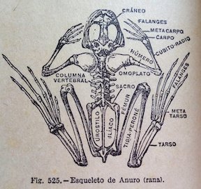
Processing data, coding, analyzing, modeling… these tasks form the core of my everyday work and are what generates my excitement and passion for research. But once a new result has come up, or a new hypothesis has been formed, how boring would it be to keep it for myself? Science is all about communication, exchanges with our peers, with stakeholders, and with the general public. Graphical representations have always been supported in research throughout the history of sciences, and particularly the life sciences (Figure 1).

I have come to realize how much I enjoy this aspect of my work, and also how much I wish I was better prepared for it! In this blogpost I will talk about visual communication in science, and tackle the question of how to make our plots, diagrams, powerpoints, figures, maps, etc. convey information that goes beyond any spoken language? I have compiled a few tips from the design and infographics fields that I think could be reinvested in our scientific communication material.

*Figure 1. Illustration from anonymous biology book (credit: Katie Garrett)*

Plan, order, design

This suggestion may appear like a rather simplistic piece of advice, but any form of communication should start with a plan. What is the name of my project, the goal, and the audience? A scientific conference poster will not be created with the same design as a flyer aimed at the general public, nor will the same tools be used. Libre office powerpoint, canva, inkscape, scribus, R, plotly, GIMP… these are the open-source software I use on a regular basis but there so many more possibilities!

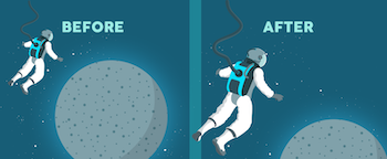
For whatever the type of visual you want to create, there are two major rules that need to be considered. First, embrace the empty space! You may think that you are wasting space that could be filled by all sorts of extremely valuable pieces of information… but this empty space has a purpose all by itself. The empty space brings forward the central elements of your design and will help focus the attention of the viewer toward them (top panel of Figure 2). Second, keep it neat and aligned. Whether you choose to anchor elements to each other or to an invisible grid, pay attention to details so that all images and text in the design from a harmonious whole (bottom panel in Figure 2).

*Figure 2. Empty spaces and alignment principles of design – examples presented by Kingcom (http://kingkom.net/12-criteres-hierarchie-visuelle/)*

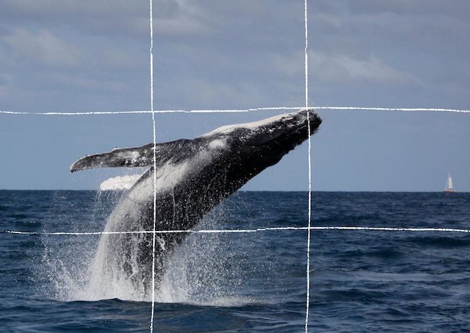
Alignment is also an essential aspect to consider when editing images. More than any text, images will provide the first impression to the viewer and may subjectively communicate ideas in an instant. To make them most effective, images may follow the ‘rule of thirds’. Imagine breaking the image down into thirds, hence creating four directive lines over it (Figure 3). Placing the points of interest of the image at the intersections or along the lines will provide balance and attract the viewer’s attention. In marine mammal science where we often use pictures of animals with the ocean as a background, aligning the horizon along one of these horizontal lines may be a good technique (which I have not followed in Figure 3 though!).

Figure 3. Rule of thirds example applied to a photo of a humpback whale calf (South Lagoon New Caledonia, credit: Opération Cétacés – Solène Derville). Notice how the tip of the calf’s jaw is at the intersection of two lines.

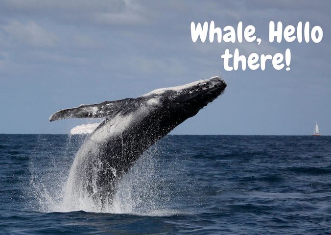
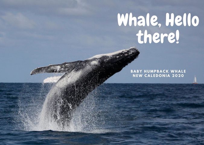
When adding text to images, it is important to not overwhelm illustrations with text by trying to use extensive written material (which happens much too often). I try to keep the text to the strict minimum and let the visuals speak for themselves. When including text over or next to an image, I place the text in the empty spaces, where the eye is drawn to (Figure 4). When using dark or contrasted images, I add a semi-transparent layer in between the text and the image to make my text pop out.

Figure 4. Text embedding example applied to a photo of a humpback whale calf (South Lagoon New Caledonia, credit: Opération Cétacés – Solène Derville). Notice how I placed the text in the empty space so that the nose of the calf would point to it.

Fonts

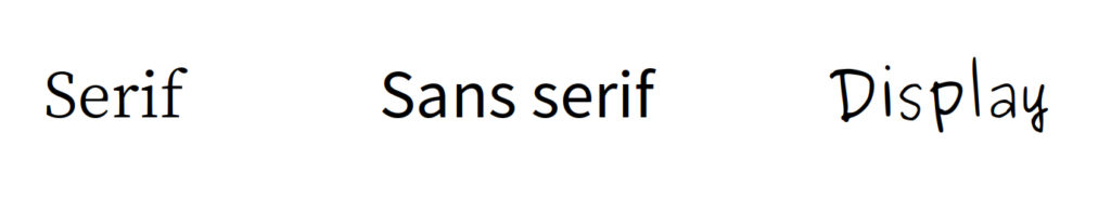
Tired of using Arial, Times and Calibri but don’t know which other font to pick? One good piece of advice I found online was to choose a font that complements the purpose of the design. To do so, it is necessary to choose the message before picking the font. There are three categories of fonts (show in Image 1):

– Serif (classic style designed for books as the little feet at the extremities of the letters guide the eye along the lines of text)

– Sans serif (designed to look clean on digital screen)

– Display (more personality, but to be used in small doses!)

I have also learned that pairing fonts together is often about using opposites (Figure 5). Contrasting fonts are complementary. For instance, it is visually appealing to combine a very bold font with a very light font, or a round font with something tall. And if you need more font choices than the ones provided by your usual software, here is a web repository to freely download thousands of different fonts: https://www.dafont.com

Figure 5. Paired fonts example applied to a photo of a humpback whale calf (South Lagoon New Caledonia, credit: Opération Cétacés – Solène Derville). Notice how I combined a rounded font with a smaller sans serif font.

Colors

Colors have inherent meaning that depends on individual cultures. Whether we want it or not, any plot, photo, or diagram that we present to an audience will carry a subliminal message depending on its color palette. So better make it fit with the message!

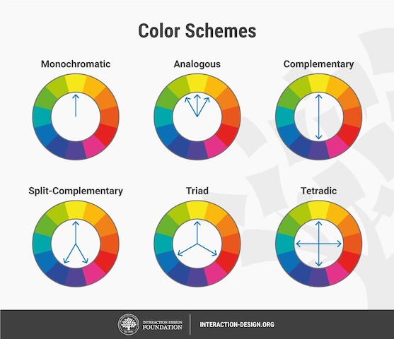
Let us go passed the boring blue shades we have used for all of our marine science presentations so far, and instead open ourselves up to an infinite choice of colors! Color nuances are defined by three things: hue (the color itself), saturation (intensity, whether the color looks more subtle or more vibrant), and value (how dark or light a color is, ranging from white to black). The color wheel helps us visualize the relationships between hues and pick the best associations (Figure 6).

Figure 6. The **color wheel** helps us visualize the relationships between hues and pick the best associations. Any of the principles above should work, from the simple monochromatic schemes to the more complex triad or tetradic schemes.

First, pick the main color, the hero color for your design. Choose a cool color (blues and greens) if you want to provide a calming impression or a warm color (reds and yellows) for something more energizing. This basic principle of color theory made me think back on the black/blue dark shaded presentations that I might have attended in the past and had trouble staying awake!

Now, create your color palette, which are the three to four colors that will compose your design, ideally combining some vibrant and some more neutral colors for contrast. For instance, in a publication, a color palette may be used consistently in all plots or figures to represent a set of variables, study areas, or species . Now how do you pick the right complementary colors? The color wheel provides you with a few basic principles that should help you choose a palette (Figure 6). From monochromatic to tetradic schemes, the choice is up to you:

– monochromatic colors: varying values or saturation of a given color picked in the wheel

– analogous colors: colors sitting next to each other in the wheel

– complementary color: colors sitting opposite to each other

If you are an R user, there are a myriad of color palettes available to produce your visuals. One of the most comprehensive list I have found was compiled by Emil Hvitfeldt in github (https://github.com/EmilHvitfeldt/r-color-palettes). For discrete color palettes, I enjoy using the Canva palettes, which are available both in the Canva designs and in R using the ‘canva’ library in combination with the ‘ggplot2’ library (https://www.canva.com/learn/100-color-combinations/).

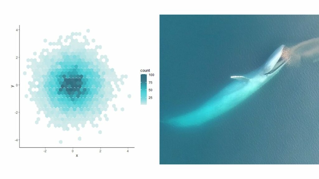
In practice, this means I can produce R plots or maps with color codes that match those I use in my canva presentations or posters. And finally, thumbs up to Dawn and Clara for creating our very own GEMM lab color palette based on whale photos collected in the field (Figure 7: https://github.com/dawnbarlow/musculusColors)!

*Figure 7: Example of a R plot colored with the musculusColors package using the blue whale “Bmlunge” palette (credit: Dawn Barlow & Clara Bird*)

I hope these few tips help you make your science as look as pretty as it is in your mind!

Sources:

A lot of the material in this blog post was inspired by the free tutorials provided by Canva: https://designschool.canva.com/courses/graphic-design-basics/?lesson=design-to-communicate

About the rule of thirds: https://digital-photography-school.com/rule-of-thirds/

About alignment: https://blog.thepapermillstore.com/design-principles-alignment/

Data Wrangling to Assess Data Availability: A Data Detective at Work

By Alexa Kownacki, Ph.D. Student, OSU Department of Fisheries and Wildlife, Geospatial Ecology of Marine Megafauna Lab

Data wrangling, in my own loose definition, is the necessary combination of both data selection and data collection. Wrangling your data requires accessing then assessing your data. Data collection is just what it sounds like: gathering all data points necessary for your project. Data selection is the process of cleaning and trimming data for final analyses; it is a whole new bag of worms that requires decision-making and critical thinking. During this process of data wrangling, I discovered there are two major avenues to obtain data: 1) you collect it, which frequently requires an exorbitant amount of time in the field, in the lab, and/or behind a computer, or 2) other people have already collected it, and through collaboration you put it to a good use (often a different use then its initial intent). The latter approach may result in the collection of so much data that you must decide which data should be included to answer your hypotheses. This process of data wrangling is the hurdle I am facing at this moment. I feel like I am a data detective.

Data wrangling illustrated by members of the R-programming community. (Image source: R-bloggers.com)

My project focuses on assessing the health conditions of the two ecotypes of bottlenose dolphins between the waters off of Ensenada, Baja California, Mexico to San Francisco, California, USA between 1981-2015. During the government shutdown, much of my data was inaccessible, seeing as it was in possession of my collaborators at federal agencies. However, now that the shutdown is over, my data is flowing in, and my questions are piling up. I can now begin to look at where these animals have been sighted over the past decades, which ecotypes have higher contaminant levels in their blubber, which animals have higher stress levels and if these are related to geospatial location, where animals are more susceptible to human disturbance, if sex plays a role in stress or contaminant load levels, which environmental variables influence stress levels and contaminant levels, and more!

Alexa, alongside collaborators, photographing transiting bottlenose dolphins along the coastline near Santa Barbara, CA in 2015 as part of the data collection process. (Image source: Nick Kellar).

Over the last two weeks, I was emailed three separate Excel spreadsheets representing three datasets, that contain partially overlapping data. If Microsoft Access is foreign to you, I would compare this dilemma to a very confusing exam question of “matching the word with the definition”, except with the words being in different languages from the definitions. If you have used Microsoft Access databases, you probably know the system of querying and matching data in different databases. Well, imagine trying to do this with Excel spreadsheets because the databases are not linked. Now you can see why I need to take a data management course and start using platforms other than Excel to manage my data.

A visual interpretation of trying to combine datasets being like matching the English definition to the Spanish translation. (Image source: Enchanted Learning)

In the first dataset, there are 6,136 sightings of Common bottlenose dolphins (Tursiops truncatus) documented in my study area. Some years have no sightings, some years have fewer than 100 sightings, and other years have over 500 sightings. In another dataset, there are 398 bottlenose dolphin biopsy samples collected between the years of 1992-2016 in a genetics database that can provide the sex of the animal. The final dataset contains records of 774 bottlenose dolphin biopsy samples collected between 1993-2018 that could be tested for hormone and/or contaminant levels. Some of these samples have identification numbers that can be matched to the other dataset. Within these cross-reference matches there are conflicting data in terms of amount of tissue remaining for analyses. Sorting these conflicts out will involve more digging from my end and additional communication with collaborators: data wrangling at its best. Circling back to what I mentioned in the beginning of this post, this data was collected by other people over decades and the collection methods were not standardized for my project. I benefit from years of data collection by other scientists and I am grateful for all of their hard work. However, now my hard work begins.

The cutest part of data wrangling: finding adorable images of bottlenose dolphins, photographed during a coastal survey. (Image source: Alexa Kownacki).

There is also a large amount of data that I downloaded from federally-maintained websites. For example, dolphin sighting data from research cruises are available for public access from the OBIS (Ocean Biogeographic Information System) Sea Map website. It boasts 5,927,551 records from 1,096 data sets containing information on 711 species with the help of 410 collaborators. This website is incredible as it allows you to search through different data criteria and then download the data in a variety of formats and contains an interactive map of the data. You can explore this at your leisure, but I want to point out the sheer amount of data. In my case, the OBIS Sea Map website is only one major platform that contains many sources of data that has already been collected, not specifically for me or my project, but will be utilized. As a follow-up to using data collected by other scientists, it is critical to give credit where credit is due. One of the benefits of using this website, is there is information about how to properly credit the collaborators when downloading data. See below for an example:

Example citation for a dataset (Dataset ID: 1201):

Lockhart, G.G., DiGiovanni Jr., R.A., DePerte, A.M. 2014. Virginia and Maryland Sea Turtle Research and Conservation Initiative Aerial Survey Sightings, May 2011 through July 2013. Downloaded from OBIS-SEAMAP (http://seamap.env.duke.edu/dataset/1201) on xxxx-xx-xx.

Citation for OBIS-SEAMAP:

Halpin, P.N., A.J. Read, E. Fujioka, B.D. Best, B. Donnelly, L.J. Hazen, C. Kot, K. Urian, E. LaBrecque, A. Dimatteo, J. Cleary, C. Good, L.B. Crowder, and K.D. Hyrenbach. 2009. OBIS-SEAMAP: The world data center for marine mammal, sea bird, and sea turtle distributions. Oceanography 22(2):104-115

Another federally-maintained data source that boasts more data than I can quantify is the well-known ERDDAP website. After a few Google searches, I finally discovered that the acronym stands for Environmental Research Division’s Data Access Program. Essentially, this the holy grail of environmental data for marine scientists. I have downloaded so much data from this website that Excel cannot open the csv files. Here is yet another reason why young scientists, like myself, need to transition out of using Excel and into data management systems that are developed to handle large-scale datasets. Everything from daily sea surface temperatures collected on every, one-degree of latitude and longitude line from 1981-2015 over my entire study site to Ekman transport levels taken every six hours on every longitudinal degree line over my study area. I will add some environmental variables in species distribution models to see which account for the largest amount of variability in my data. The next step in data selection begins with statistics. It is important to find if there are highly correlated environmental factors prior to modeling data. Learn more about fitting cetacean data to models here.

The ERDAPP website combined all of the average Sea Surface Temperatures collected daily from 1981-2018 over my study site into a graphical display of monthly composites. (Image Source: ERDDAP)

As you can imagine, this amount of data from many sources and collaborators is equal parts daunting and exhilarating. Before I even begin the process of determining the spatial and temporal spread of dolphin sightings data, I have to identify which data points have sex identified from either hormone levels or genetics, which data points have contaminants levels already quantified, which samples still have tissue available for additional testing, and so on. Once I have cleaned up the datasets, I will import the data into the R programming package. Then I can visualize my data in plots, charts, and graphs; this will help me identify outliers and potential challenges with my data, and, hopefully, start to see answers to my focal questions. Only then, can I dive into the deep and exciting waters of species distribution modeling and more advanced statistical analyses. This is data wrangling and I am the data detective.

What people may think a ‘data detective’ looks like, when, in reality, it is a person sitting at a computer. (Image source: Elder Research)

Like the well-known phrase, “With great power comes great responsibility”, I believe that with great data, comes great responsibility, because data is power. It is up to me as the scientist to decide which data is most powerful at answering my questions.

Plan, order, design

Fonts

Colors

Sources:

Share this:

Share this: