El Niño de Navidad: What is atmospheric Santa Claus bringing to Oregon krill and whales?

By Rachel Kaplan, PhD student, Oregon State University College of Earth, Ocean, and Atmospheric Sciences and Department of Fisheries, Wildlife, and Conservation Sciences, Geospatial Ecology of Marine Megafauna Lab

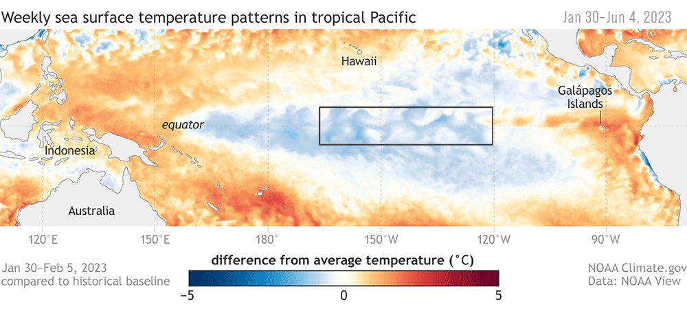
Early June marked the onset of El Niño conditions in the Pacific Ocean , which have been strengthening through the fall and winter. For Oregonians, this climate event means unseasonably warm December days, less snow and overall precipitation (it’s sunny as I write this!), and the potential for increased wildfires and marine heatwaves next summer.

This phenomenon occurs about every two to seven years as part of the El Niño Southern Oscillation (ENSO), a cyclical rotation of atmospheric and oceanic conditions in the Pacific Ocean that is initiated by departures from and returns to “normal conditions” at the equator. Typically, the trade winds blow warm water west along the equator, and El Niño occurs when these winds weaken or reverse. As a result, the upwelling of cold water at the equator ceases, and warm water flows towards the west coast of the Americas, rather than its typical pathway towards Asia. When the trade winds resume their normal direction, usually after months or a year, the system returns to “normal” conditions – or, it can enter the cool La Niña part of the cycle, in which the trade winds are stronger than normal. “El Niño de Navidad” was named by South American fisherman in the 1600s because this event tends to peak in December – and El Niño is clearly going to be a guest for Christmas this year.

Figure 1. Maps of sea surface temperature anomalies show Pacific Ocean conditions during a strong La Niña (top) and El Niño (bottom). Source: NOAA climate.gov

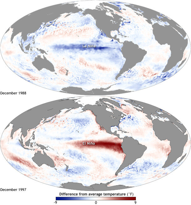
These events at the equator trigger changes in global atmospheric circulation patterns, and they can shape weather around the world. Teleconnection, the coherence between meteorological and environmental phenomena occurring far apart, is to me one of the most incredible things about the natural world.  This coherence means that the biological community off the Oregon coast is strongly impacted by events initiated at the equator, with consequences that we don’t yet fully understand.

The effects of El Niño are diverse – floods in some places, droughts in others – and their onset can mean wildly different things for Oregon, Peru, Alaska, and beyond. As we tap our fingers waiting to be able to ski and snowboard in Oregon, what does our current El Niño event mean for the life in the waters off our coast?

Figure 2. Anomalous conditions at the equator qualified as an El Niño event in June 2023.

ENSO plays a big role in the variability in our local Northern California Current (NCC) system, and the outcomes of these events can differ based on the strength and how the signal propagates through the ocean and atmosphere (Checkley & Barth, 2009). Large-scale “coastal-trapped” waves flowing alongshore can bring the warm water signal of an El Niño to our ocean backyard in a matter of weeks. One of the first impacts is a deepening of the thermocline, the upper ocean’s steep gradient in temperature, which changes the cycling of important nutrients in the surface ocean. This can result in a decrease in upwelling and primary productivity that sends ramifications through the food web, including consequences for grazers and predators like zooplankton, marine mammals, and seabirds (Checkley & Barth, 2009).

In addition to these ecosystem effects that result from local changes, the ocean community can also receive new visitors from afar, and see others flee . For krill, the shrimp-like whale prey that I spend a lot of my time thinking about, community composition can change as subtropical species typically found off southern and Baja California are displaced by horizontal ocean flow, or as resident species head north (Lilly & Ohman, 2021).

Figure 3. This Euphausia gibboides krill is typically found in offshore subtropical habitats but moves north and inshore during El Niño events, and tends to persist awhile in these new environments, impacting the local zooplankton community. Source: Solvn Zankl

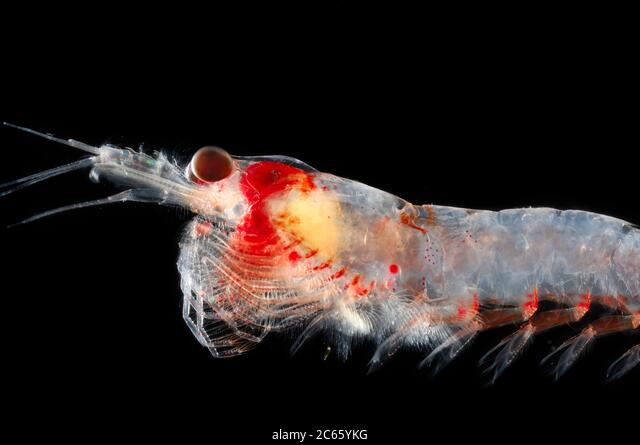
The two main krill species that occur in the NCC, Euphausia pacifica and Thysanoessa spinifera, favor the cool, coastal waters typical off the coast of Oregon. During El Niño events, E. pacifica tends to contract its distribution inshore in order to continue occupying these conditions, increasing its spatial overlap with T. spinifera (Lilly & Ohman, 2021). In addition, both tend to shift their populations north, toward cooler, upwelling waters (Lilly & Ohman, 2021).

These krill species are a favored prey of rorqual whales, and the coast of Oregon is an important foraging ground for humpback, blue, and fin whales. Predators tend to follow their prey, and shifting distributions of these krill species may cause whales to move, too. During the 2014-2015 “Blob” event in the Pacific Ocean, a marine heatwave was exacerbated by El Niño conditions. Humpback whales in central California shifted their distributions inshore in response to sparse offshore krill, increasing their overlap with fishing gear and leading to an increase in entanglement events (Santora et al., 2020). Further north, these conditions even led humpback whales to forage in the Columbia River!

Figure 4. In September 2015, El Niño conditions led humpback whales to follow their prey and forage in the Columbia River.

As El Niño events compound with the impacts of global climate change, we can expect these distributional shifts – and perhaps surprises – to continue. By the year 2100, the west coast habitat of both T. spinifera and E. pacifica will likely be constrained due to ocean warming – and when El Niños occur, this habitat will decrease even further (Lilly & Ohman, 2021). As a result, the abundances of both species are expected to decrease during El Niño events, beyond what is seen today (Lilly & Ohman, 2021). This decline in prey availability will likely present a problem for future foraging whales, which may already be facing increased environmental challenges.

Understanding connections is inherent to the field of ecology, and although these environmental dependencies are part of what makes life so vulnerable, they can also be a source of resilience. Although humans have known about ENSO for over 400 years, the complex interplay between nature, anthropogenic systems, and climate change means that we are still learning the full implications of these events. Just as waiting for Santa Claus always keeps kids guessing, the dynamic ocean keeps surprising us, too.

Loading

References

Checkley, D. M., & Barth, J. A. (2009). Patterns and processes in the California Current System. Progress in Oceanography, 83(1–4), 49–64. https://doi.org/10.1016/j.pocean.2009.07.028

Lilly, L. E., & Ohman, M. D. (2021). Euphausiid spatial displacements and habitat shifts in the southern California Current System in response to El Niño variability. Progress in Oceanography, 193, 102544. https://doi.org/10.1016/j.pocean.2021.102544

Santora, J. A., Mantua, N. J., Schroeder, I. D., Field, J. C., Hazen, E. L., Bograd, S. J., Sydeman, W. J., Wells, B. K., Calambokidis, J., Saez, L., Lawson, D., & Forney, K. A. (2020). Habitat compression and ecosystem shifts as potential links between marine heatwave and record whale entanglements. Nat Commun, 11(1), 536. https://doi.org/10.1038/s41467-019-14215-w


Zooming in: A closer look at bottlenose dolphin distribution patterns off of San Diego, CA

By: Alexa Kownacki, Ph.D. Student, OSU Department of Fisheries and Wildlife, Geospatial Ecology of Marine Megafauna Lab

Data analysis is often about parsing down data into manageable subsets. My project, which spans 34 years and six study sites along the California coast, requires significant data wrangling before full analysis. As part of a data analysis trial, I first refined my dataset to only the San Diego survey location. I chose this dataset for its standardization and large sample size; the bulk of my sightings, over 4,000 of the 6,136, are from the San Diego survey site where the transect methods were highly standardized. In the next step, I selected explanatory variable datasets that covered the sighting data at similar spatial and temporal resolutions. This small endeavor in analyzing my data was the first big leap into understanding what questions are feasible in terms of variable selection and analysis methods. I developed four major hypotheses for this San Diego site.

The study species: common bottlenose dolphin (Tursiops truncatus) seen along the California coastline in 2015. Image source: Alexa Kownacki.

Hypotheses:

H1: I predict that bottlenose dolphin sightings along the San Diego transect throughout the years 1981-2015 exhibit clustered distribution patterns as a result of the patchy distributions of both the species’ preferred habitats, as well as the social nature of bottlenose dolphins.

H2: I predict there would be higher densities of bottlenose dolphin at higher latitudes spanning 1981-2015 due to prey distributions shifting northward and less human activities in the northerly sections of the transect.

H3: I predict that during warm (positive) El Niño Southern Oscillation (ENSO) months, the dolphin sightings in San Diego would be distributed more northerly, predominantly with prey aggregations historically shifting northward into cooler waters, due to (secondarily) increasing sea surface temperatures.

H4: I predict that along the San Diego coastline, bottlenose dolphin sightings are clustered within two kilometers of the six major lagoons, with no specific preference for any lagoon, because the murky, nutrient-rich waters in the estuarine environments are ideal for prey protection and known for their higher densities of schooling fishes.

Data Description:

The common bottlenose dolphin (Tursiops truncatus) sighting data spans 1981-2015 with a few gap years. Sightings cover all months, but not in all years sampled. The same transect in San Diego was surveyed in a small, rigid-hulled inflatable boat with approximately a two-kilometer observation area (one kilometer surveyed 90 degrees to starboard and port of the bow).

I wanted to see if there were changes in dolphin distribution by latitude and, if so, whether those changes had a relationship to ENSO cycles and/or distances to lagoons. For ENSO data, I used the NOAA database that provides positive, neutral, and negative indices (1, 0, and -1, respectively) by each month of each year. I matched these ENSO data to my month-date information of dolphin sighting data. Distance from each lagoon was calculated for each sighting.

Figure 1. Map representing the San Diego transect, represented with a light blue line inside of a one-kilometer buffered “sighting zone” in pale yellow. The dark pink shapes are dolphin sightings from 1981-2015, although some are stacked on each other and cannot be differentiated. The lagoons, ranging in size, are color-coded. The transect line runs from the breakwaters of Mission Bay, CA to Oceanside Harbor, CA.

Results: 

H1: True, dolphins are clustered and do not have a uniform distribution across this area. Spatial analysis indicated a less than a 1% likelihood that this clustered pattern could be the result of random chance (Fig. 1, z-score = -127.16, p-value < 0.0001). It is well-known that schooling fishes have a patchy distribution, which could influence the clustered distribution of their dolphin predators. In addition, bottlenose dolphins are highly social and although pods change in composition of individuals, the dolphins do usually transit, feed, and socialize in small groups.

Figure 2. Summary from the Average Nearest Neighbor calculation in ArcMap 10.6 displaying that bottlenose dolphin sightings in San Diego are highly clustered. When the z-score, which corresponds to different colors on the graphic above, is strongly negative (< -2.58), in this case dark blue, it indicates clustering. Because the p-value is very small, in this case, much less than 0.01, these results of clustering are strongly significant.

H2: False, dolphins do not occur at higher densities in the higher latitudes of the San Diego study site. The sightings are more clumped towards the lower latitudes overall (p < 2e-16), possibly due to habitat preference. The sightings are closer to beaches with higher human densities and human-related activities near Mission Bay, CA. It should be noted, that just north of the San Diego transect is the Camp Pendleton Marine Base, which conducts frequent military exercises and could deter animals.

Figure 3. Histogram comparing the latitudes with the frequency of dolphin sightings in San Diego, CA. The x-axis represents the latitudinal difference from the most northern part of the transect to each dolphin sighting. Therefore, a small difference would translate to a sighting being in the northern transect areas whereas large differences would translate to sightings being more southerly. This could be read from left to right as most northern to most southern. The y-axis represents the frequency of which those differences are seen, that is, the number of sightings with that amount of latitudinal difference, or essentially location on the transect line. Therefore, you can see there is a peak in the number of sightings towards the southern part of the transect line.

H3: False, during warm (positive) El Niño Southern Oscillation (ENSO) months, the dolphin sightings in San Diego were more southerly. In colder (negative) ENSO months, the dolphins were more northerly. The differences between sighting latitude and ENSO index was significant (p<0.005). Post-hoc analysis indicates that the north-south distribution of dolphin sightings was different during each ENSO state.

Figure 4. Boxplot visualizing distributions of dolphin sightings latitudinal differences and ENSO index, with -1,0, and 1 representing cold, neutral, and warm years, respectively.

H4: True, dolphins are clustered around particular lagoons. Figure 5 illustrates how dolphin sightings nearest to Lagoon 6 (the San Dieguito Lagoon) are always within 0.03 decimal degrees. Because of how these data are formatted, decimal degrees is the easiest way to measure change in distance (in this case, the difference in latitude). In comparison, dolphins at Lagoon 5 (Los Penasquitos Lagoon) are distributed across distances, with the most sightings further from the lagoon.

Figure 5. Bar plot displaying the different distances from dolphin sighting location to the nearest lagoon in San Diego in decimal degrees. Note: Lagoon 4 is south of the study site and therefore was never the nearest lagoon.

I found a significant difference between distance to nearest lagoon in different ENSO index categories (p < 2.55e-9): there is a significant difference in distance to nearest lagoon between neutral and negative values and positive and neutral years. Therefore, I hypothesize that in neutral ENSO months compared to positive and negative ENSO months, prey distributions are changing. This is one possible hypothesis for the significant difference in lagoon preference based on the monthly ENSO index. Using a violin plot (Fig. 6), it appears that Lagoon 5, Los Penasquitos Lagoon, has the widest variation of sighting distances in all ENSO index conditions. In neutral years, Lagoon 0, the Buena Vista Lagoon has multiple sightings, when in positive and negative years it had either no sightings or a single sighting. The Buena Vista Lagoon is the most northerly lagoon, which may indicate that in neutral ENSO months, dolphin pods are more northerly in their distribution.

Figure 6. Violin plot illustrating the distance from lagoons of dolphin sightings under different ENSO conditions. There are three major groups based on ENSO index: “-1” representing cold years, “0” representing neutral years, and “1” representing warm years. On the x-axis are lagoon IDs and on the y-axis is the distance to the nearest lagoon in decimal degrees. The wider the shapes, the more sightings, therefore Lagoon 6 has many sightings within a very small distance compared to Lagoon 5 where sightings are widely dispersed at greater distances.


Bottlenose dolphins foraging in a small group along the California coast in 2015. Image source: Alexa Kownacki.

Takeaways to science and management: 

Bottlenose dolphins have a clustered distribution which seems to be related to ENSO monthly indices, and likely, their social structures. From these data, neutral ENSO months appear to have something different happening compared to positive and negative months, that is impacting the sighting distributions of bottlenose dolphins off the San Diego coastline. More research needs to be conducted to determine what is different about neutral months and how this may impact this dolphin population. On a finer scale, the six lagoons in San Diego appear to have a spatial relationship with dolphin sightings. These lagoons may provide critical habitat for bottlenose dolphins and/or for their preferred prey either by protecting the animals or by providing nutrients. Different lagoons may have different spans of impact, that is, some lagoons may have wider outflows that create larger nutrient plumes.

Other than the Marine Mammal Protection Act and small protected zones, there are no safeguards in place for these dolphins, whose population hovers around 500 individuals. Therefore, specific coastal areas surrounding lagoons that are more vulnerable to habitat loss, habitat degradation, and/or are more frequented by dolphins, may want greater protection added at a local, state, or federal level. For example, the Batiquitos and San Dieguito Lagoons already contain some Marine Conservation Areas with No-Take Zones within their reach. The city of San Diego and the state of California need better ways to assess the coastlines in their jurisdictions and how protecting the marine, estuarine, and terrestrial environments near and encompassing the coastlines impacts the greater ecosystem.

This dive into my data was an excellent lesson in spatial scaling with regards to parsing down my data to a single study site and in matching my existing data sets to other data that could help answer my hypotheses. Originally, I underestimated the robustness of my data. At first, I hesitated when considering reducing the dolphin sighting data to only include San Diego because I was concerned that I would not be able to do the statistical analyses. However, these concerns were unfounded. My results are strongly significant and provide great insight into my questions about my data. Now, I can further apply these preliminary results and explore both finer and broader scale resolutions, such as using the more precise ENSO index values and finding ways to compare offshore bottlenose dolphin sighting distributions.