Distribution – Page 2 – Geospatial Ecology of Marine Megafauna Laboratory

Hundreds and hundreds and hundreds of models: An ecologist’s love for programming

By Dawn Barlow, PhD student, Department of Fisheries & Wildlife, Geospatial Ecology of Marine Megafauna Lab

When people hear that I study blue whales, they often ask me questions about what it’s like to be close to the largest animal on the planet, where we do fieldwork, and what data we are interested in collecting. While I love time at sea, my view on a daily basis is rarely like this:

Our small research vessel at sunset in New Zealand’s South Taranaki Bight at the end of a day of blue whale survey. Photo by D. Barlow.

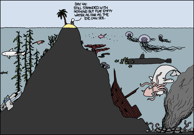
More often than not, it looks something like this:

In my application letter to Dr. Leigh Torres, I wrote something along the lines of “while I relish remote fieldwork, I also find great satisfaction in the analysis process.” This statement is increasingly true for me as I grow more proficient in statistical modeling and computer programming. When excitedly telling my family about how I am trying to model relationships between oceanography, krill, whales, and satellite imagery, I was asked what I meant by “model”. Put simply, a model is a formula or equation that we can use to describe a pattern. I have been told, “all models are wrong, but some models work.” What does this mean? While we may never know exactly every pattern of whale feeding behavior, we can use the data we have to describe some of the important relationships. If our model performance is very good, then we have likely described most of what drives the patterns we see. If model performance is poor, then there is more to the pattern that we have not yet captured in either our data collection or in our analytical methods. Another common saying about models is, “A model is only ever as good as the data you put into it.” While we worked hard during field seasons to collect a myriad of data about what could be influencing blue whale distribution patterns, we inevitably could not capture everything, nor do we know everything that should be measured.

So, how do you go about finding the ‘best’ model? This question is what I’ve been grappling with over the last several weeks. My goal is to describe the patterns in the krill that drive patterns in whale distribution, the patterns in oceanography that drive patterns in the krill, and the patterns in the oceanography that drive patterns in whale distribution. The thing is, we have many metrics to describe oceanographic patterns (surface temperature, mixed layer depth, strength of the thermocline, integral of fluorescence, to name just a few), as well as several metrics to describe the krill (number of aggregations, aggregation density, depth, and thickness). When I multiplied out how many possible combinations of predictor variables and parameters we’re interested in modeling, I realized this meant running nearly 300 models in order to settle on the best ten. This is where programming comes in, I told myself, and caught my breath.

I’ve always loved languages. When I was much younger, I thought I might want to study linguistics. As a graduate student in wildlife science, the language I’ve spent the most time learning, and come to love, is the statistical programming language R. Just like any other language, R has syntax and structure. Like any other language, there are many ways in which to articulate something, to make a particular point or reach a particular end goal. Well-written code is sometimes described as “elegant”, much like a well-articulated piece of writing. While I certainly do not consider myself “fluent” in R, it is a language I love learning. I like to think that the R scripts I write are an attempt to eloquently uncover and describe ecological patterns.

Rather than running 300 models one by one, I wrote an R script to run many models at a time, and then sort the outputs by model performance. I may look at the five best models of 32 options in order to select one. But this is where Leigh reminds me to step back from the programming for a minute and put my ecologist hat back on. Insight on the part of the modeler is needed in order to discern between what are real ecological relationships and what are spurious correlations in the data. It may not be quite as simple as choosing the model with the highest explanatory power when my goal is to make ecological inferences.

So, where does this leave me? Hundreds of models later, I am still not entirely sure which ones are best, although I’ve narrowed it down considerably. My programming proficiency and confidence continue to grow, but that only goes so far in ecology. Knowledge of my study system is equally important. So my workflow lately goes something like this: write code, try to interpret model outputs, consider what I know about the oceanography of my study region, re-write code, re-interpret the revised results, and so on. Hopefully this iterative process is bringing us gradually closer to an understanding of the ecology of blue whales on a foraging ground… stay tuned.

A blue whale lunges on an aggregation of krill in New Zealand’s South Taranaki Bight. Drone piloted by Todd Chandler.

Albatrosses at sunrise, dolphins at sunset: Northern California Current cruise

By Dawn Barlow, PhD student, Geospatial Ecology of Marine Megafauna Lab, Department of Fisheries and Wildlife, Oregon State University

Sun on my face and wind in my hair, scanning the expanse of blue. Forty minutes on, twenty minutes off, from sunrise until sunset, day after day. Hours of seemingly empty blue, punctuated by graceful black-footed albatrosses wheeling and gliding over the swells, by the splashing approach of a curious group of Pacific white-sided dolphins coming to play in the bow of the ship, by whale spouts on the horizon and the occasional breaching humpback. A flurry of data entry—geographic coordinates, bearing and distance from the ship, number of animals, species identification, behavior—and then back to blue.

Scanning for marine mammals from the flying bridge of NOAA ship Bell M. Shimada. Photo: Jess O’Loughlin.

I’ve just returned from the Northern California Current (NCC) ecosystem cruise aboard NOAA ship Bell M. Shimada. My role on board was the marine mammal observer, logging marine mammal sightings during the transits between sampling stations. We surveyed and sampled between Cape Mears, Oregon and Trinidad, California, from right along the coast out to 200 nautical miles offshore. Resources in the marine environment are patchy, and our coastline is highly productive. This diversity in environmental conditions creates niche habitats for many species, which is one reason why surveying and sampling across a broad geographic range can be so informative. We left Newport surrounded by gray whales, feeding in green, chilly waters at temperatures around 12°C. Moving west, the marine mammal and seabird sightings were increasingly sparse, the water increasingly blue, and the surface temperature warmed to a balmy 17°C. We had reached offshore waters, an ocean region sometimes referred to as the “blue desert”. For an entire day I didn’t see a single marine mammal and only just a few seabirds, until a handful of common dolphins—more frequently seen in warm-temperate and tropical waters to the south—joined the ship at sunset. As we transited back inshore over the productive Heceta Bank, the water became cooler and greener. I stayed busy logging sightings of humpback and gray whales, harbor porpoise and Dall’s porpoise, pacific white-sided dolphins and sea lions. These far-ranging marine predators must find a way to make a living in the patchy and dynamic ocean environment, and therefore their distribution is also patchy—aggregated around areas of high productivity and prey availability, and occasionally seen transiting in between.

Here are a few cruise highlights:

Curious groups of common dolphins (Delphinus delphis) came to play in the bow wake of the ship and even checked out the plankton nets when they were deployed. Common dolphins are typically found further south, however we saw several groups of them in the warmer waters far offshore.

Common dolphins (Delphinus delphis). Photo: Dawn Barlow.

Ocean sunfish (Mola mola) will occasionally lay themselves flat at the surface so that seabirds will pick them clean of any parasites. I was delighted to observe this for the first time just off Newport! There were several more sunfish sightings throughout the cruise.

Gull picking parasites off an ocean sunfish (Mola mola). Photo: Dawn Barlow.

A masked booby (Sula dactylatra) hung around the ship for a bit, 16 nautical miles from shore, just south of the Oregon-California border. Considered a tropical species, a sighting this far north is extremely rare. While masked boobies are typically distributed in the Caribbean and tropical Pacific from Mexico to Australia, one found its way to the Columbia River in 2006 (first record in the state of Oregon) and another showed up here to Newport in 2015 – reportedly only the second to be recorded north of Mendocino County, California. Perhaps this sighting is the third?

Masked booby (Sula dactylatra). Photo: Dawn Barlow.

While most of my boat-based fieldwork experiences have been focused on marine mammal research, this was an interdisciplinary cruise aimed at studying multiple aspects of the northern California current ecosystem. There were researchers on board studying oceanography, phytoplankton and harmful algal blooms, zooplankton, and microplastics. When a group of enthusiastic scientists with different areas of expertise come together and spend long days at sea, there is a wonderful opportunity to learn from one another. The hydroacoustic backscatter on the scientific echosounder prompted a group discussion about vertical migration of plankton one evening. Another evening I learned about differences in energetic content between krill species, and together we mused about what that might mean for marine predators. This is how collaborations are born, and I am grateful for the scientific musings with so many insightful people.

Thank you to the Shimada crew and the NCC science team for a wonderful cruise!

The NCC science team after a successful cruise!

Cloudy with a chance of blue whales

By Dawn Barlow, PhD student, Department of Fisheries & Wildlife, Geospatial Ecology of Marine Megafauna Lab

As a PhD student studying the ecology of blue whales in New Zealand, my time is occupied by questions such as: When and where are the blue whales? Can we predict where they will be based on environmental conditions? How does their distribution overlap with human activity such as oil and gas exploration?

Leigh and I have just returned from New Zealand, where I gave an oral presentation at the Society for Conservation Biology Oceania Congress entitled “Cloudy with a chance of whales: Forecasting blue whale presence to mitigate industrial impacts based on tiered, bottom-up models”. While the findings I presented are preliminary, an exciting ecological story is emerging, and one with clear management implications.

The South Taranaki Bight (STB) region of New Zealand is an important area for a population of blue whales which are unique to New Zealand. A wind-driven upwelling system brings cold, productive waters into the bight [1], which sustains high densities of krill [2], blue whale prey. The region is also frequented by busy shipping traffic, oil and gas drilling and extraction platforms as well as seismic survey effort for subsurface oil and gas reserves, and is the site of a recently-permitted seabed mine for iron sands (Fig. 1). However, a lack of knowledge on blue whale distribution and habitat use patterns has impeded effective management of these potential anthropogenic threats.

Figure 1. A blue whale surfaces in front of a floating production storage and offloading vessel servicing the oil rigs in the South Taranaki Bight. Photo by D. Barlow.

Three surveys were conducted in the STB region in the summer months of 2014, 2016, and 2017. During that time, we not only looked for blue whales, we also collected oceanographic data and hydroacoustic backscatter data to map and measure aspects of the krill in the region. These data streams will help us understand the functional, ecological relationships between the environment (oceanography), prey (krill), and predators (blue whales) in the ecosystem (Fig. 2). But in practice these data are costly and time-consuming to collect, while other data sources such as satellite imagery are readily accessible to managers at a variety of spatial and temporal scales. Therefore, another one of my aims is to link the data we collected in the field to satellite imagery, so that managers can have a practical tool to predict when and where the blue whales are most likely to be found in the region.

Figure 2. Data streams collected during surveys of the South Taranaki Bight Region in 2014, 2016, and 2017.

So what did I find? Here are the highlights from my preliminary analyses:

The majority of the patterns in blue whale distribution can be explained by the density, depth, and thickness of the krill patches.
Patterns in the krill are driven by oceanography.
Those same oceanographic parameters that drive the krill can be used to explain blue whale distribution.
There are tight relationships between the important oceanographic variables and satellite images of sea surface temperature.
Blue whale distribution can, to some degree, be explained using just satellite imagery.

We were able to identify a sea surface temperature range in the satellite imagery of approximately 18°C where the likelihood of finding a blue whale is the highest. Is this because blue whales really like 18° water? Well, more likely this relationship exists because the satellite imagery is reflective of the oceanography, and the oceanography drives patterns in the krill distribution, and the krill drives the distribution of blue whales (Fig. 3). We were able to make each of these functional linkages through our series of models, which is quite exciting.

Figure 3. The tiered modeling approach we took to investigate the ecological relationships between blue whales, krill, oceanography, and satellite imagery. Because of the ecological linkages we made, we are able to say that any relationship between whale distribution and satellite imagery most likely reflects a relationship between the blue whales and their prey.

That’s all well and good, but we were interested in testing these relationships to see if our identified habitat associations hold up even when we do not have field data (oceanographic, krill, and whale data). This past austral summer, we did not have a field season to collect data, but there was a large seismic airgun survey of the STB region. Seismic survey vessels are required to have trained marine mammal observers on board, and we were given access to the blue whale sightings data they recorded during the survey. In December, when the water was right around the preferred temperature identified by our models (18°C), the observers made 52 blue whale sightings (Fig. 4). In January and February, the waters warmed and only two sightings were made in each month. This is not only reassuring because it supports our model results, it also implies that there is the potential to balance industrial use of the area with protection of blue whale habitat, based on our understanding of the ecology. In January and February, very few blue whales were likely disturbed by the industrial activity in the STB, as conditions were not favorable for foraging at the location of the seismic survey. In contrast, the blue whales that were in the STB region in December may have experienced physiological consequences of sustained exposure to airgun noise since the conditions were favorable for foraging in the STB. In other words, the whales may have tolerated the noise exposure to gain access to good food, but this could have significant biological repercussions such as increased stress [3].

Figure 4. Monthly sea surface temperature (MODIS Aqua) overlaid with blue whale sightings from marine mammal observers aboard seismic survey vessel R/V Amazon Warrior. Black rectangles represent areas of seismic survey effort. Blue whale sighting location data were provided by RPS Energy Pty Ltd & Schlumberger, and Todd Energy.

In the first two weeks of July, we presented these latest findings to managers at the New Zealand Department of Conservation, the Minister of Conservation, the CEO and Policy Advisor of a major oil and gas conglomerate, NGOs, advocacy groups, and scientific colleagues. It was valuable to gather feedback from many different stakeholders, and satisfying to see such a clear interest in, and management application of, our work.

Dr. Leigh Torres and Dawn Barlow in front of Parliament in Wellington, New Zealand, following the presentation of their recent findings.

What’s next? We’re back in Oregon, and diving back into analysis. We intend to take the modeling work a step further to make the models predictive—for example, can we forecast where the blue whales will be based on the temperature, productivity, and winds two weeks prior? I am excited to see where these next steps lead!

References:

Shirtcliffe TGL, Moore MI, Cole AG, Viner AB, Baldwin R, Chapman B. 1990 Dynamics of the Cape Farewell upwelling plume, New Zealand. New Zeal. J. Mar. Freshw. Res. 24, 555–568. (doi:10.1080/00288330.1990.9516446)
Bradford-Grieve JM, Murdoch RC, Chapman BE. 1993 Composition of macrozooplankton assemblages associated with the formation and decay of pulses within an upwelling plume in greater cook strait, New Zealand. New Zeal. J. Mar. Freshw. Res. 27, 1–22. (doi:10.1080/00288330.1993.9516541)
Rolland RM, Parks SE, Hunt KE, Castellote M, Corkeron PJ, Nowacek DP, Wasser SK, Kraus SD. 2012 Evidence that ship noise increases stress in right whales. Proc. Biol. Sci. 279, 2363–8. (doi:10.1098/rspb.2011.2429)

Oregon sea otter reintroduction: opinions, perspectives, and theories

By Dominique Kone, Masters Student in Marine Resource Management

Species reintroductions can be hotly contested issues because they can negatively impact other species, ecosystems, and society, as well as failing, altogether. The uncertainty of their outcomes forces stakeholder groups to form their own opinions on whether it’s a good idea to proceed with a reintroduction. When you have several groups with conflicting values and views, managers need to focus on the information most important for them to make a well-informed decision on whether to pursue a reintroduction.

As researchers, we can play an important role by carefully considering and addressing these views through our research, if the appropriate data is available. Despite being in the early days of our study on the potential sea otter reintroduction to Oregon, we have already heard several perspectives regarding its potential success, the type of research we should do, and if sea otters should be brought back to Oregon. Here, I present some of the most interesting and relevant opinions, perspectives, and theories I’ve heard regarding this reintroduction idea.

The first reintroduction failed because of X, Y, and Z.

From 1970-1971, managers translocated 93 sea otters to Oregon in a reintroduction effort (Jameson et al. 1982). However, in a matter of 5-6 years, all sea otters disappeared, and the effort was considered a failure. Researchers have theorized that sea otters left Oregon due to a lack of suitable habitat and prey, or to return home to sites from which they were captured. Others have reasoned that managers should have introduced southern sea otters instead of northern sea otters, suggesting one subspecies’ genetic pre-disposition may improve their chance for survival.

Knowing the reasons for this failure may help managers avoid these causes in a future reintroduction attempt and increase its chance of success. We, as scientists, can also gain insight from knowing these causes because this may help us better tailor our research to potentially investigate whether those causes still pose a threat to sea otters during a second attempt. Unfortunately, we lack concrete evidence on what exactly caused this failure, but we can still work to test some these theories.

An otter is an otter, no matter where you put it.

There is evidence that northern and southern sea otters are genetically distinct, to a certain degree (Valentine et al. 2008, Larson et al. 2012), and hypotheses have been put forward that the two subspecies may be behaviorally- and ecologically-distinct, too. Studies have shown that northern and southern sea otters have different sized and shaped skulls and teeth, which researchers hypothesize may be a specialized foraging adaptation for consuming different prey species (Campbell & Santana 2017, Timm-Davis et al. 2015). This view suggests that each subspecies has developed unique traits to adapt to the environmental conditions specific to their current ranges. Therefore, when considering which subspecies to bring to Oregon, managers should reintroduce the subspecies with traits better-suited to cope with the types of habitat, prey assemblages, and oceanographic conditions specific to Oregon.

However, other scientists hold the opposite view, and argue that “an otter is an otter” no matter where you put it. This perspective suggests that both subspecies have an equal chance at surviving in any type of suitable habitat because all otters behave in similar ways. Therefore, ecologically, it may not matter which subspecies managers bring to Oregon.

Oregon doesn’t have enough sea otter habitat.

Kelp is considered important sea otter habitat. In areas with high sea otter densities, such as central and southern California, kelp forests are persistent throughout the year. However, in Oregon, our kelp primarily consists of bull kelp – a slightly more fragile species compared to the durable giant kelp in California. In winter, this bull kelp gets dislodged during intense storms, resulting in seasonal changes in kelp availability. Managers worry that this seasonality could reduce the amount of suitable habitat, to the point where Oregon may not be able to support sea otters.

Yet, we know sea otters used to exist here; therefore, we can assume there must have been some suitable habitat that may persist today. Furthermore, sea otters use a range of habitats, including estuaries, bays, and reefs (Laidre et al. 2009, Lafferty & Tinker 2014, Kvitek et al. 1988). Therefore, even during times when kelp is less abundant, sea otters could use these other forms of habitat along the Oregon coast. Luckily, we have the spatial tools and data to assess how much, where, and when we have suitable habitat, and I will specifically address this in my thesis.

They’ll eat everything!

Sea otters are famous for their voracious appetites for benthic invertebrates, some of which are of commercial and recreational importance to nearshore fisheries. In some cases, sea otters have significantly reduced prey densities, such as sea urchins and Dungeness crab (Garshelis & Garshelis 1984, Estes & Palmisano 1974). However, without a formal analysis, it’s difficult to know if sea otters will have similar impacts on Oregon’s nearshore species, as well as at spatial scale these impacts will occur and whether our fisheries will be affected. We can predict where sea otters are likely to occur based on the presence of suitable habitat, but foraging impacts could be more localized or widespread across sea otter’s entire potential range. To better anticipate these impacts, managers will need an understanding of how much sea otters eat, where foraging could occur based on the availability of prey, and where sea otters and fisheries are likely to interact. I will also address this concern in my thesis.

To reintroduce or not to reintroduce? That is the question.

I have found that many scientists and managers have strong opinions on whether it’s appropriate to bring sea otters back to Oregon. Those who argue against a reintroduction often highlight many of the theories already mentioned here – lack of habitat, potential impacts to fisheries, and genetics. While other opponents provided more logistical and practical justifications, such as confounding politics, as well as difficulties in getting public support and regulatory permission to move a federally-listed species.

In contrast, proponents of this idea argue that a reintroduction could augment the recovery of the species by providing additional habitat for the species to rebound to pre-exploitation levels, as well as allowing for increased gene flow between southern and northern sea otter populations. Other proponents have brought up potential benefits to humans, such restoring ecosystem services, providing an economic boost through tourism, or preserving tribal and cultural connections. Such benefits may be worth attempting another reintroduction effort.

As you can see, there are several opinions and perspectives related to a potential sea otter reintroduction to Oregon. While it’s important to consider all opinions, managers still need facts to make key decisions. Scientists can play an important role in providing this information, so managers can make a well-informed decision. Oregon managers have not yet decided whether to proceed with a sea otter reintroduction, but our lab is working to provide them with reliable and accurate science, so they may form their own opinions and arrive at their own decision.

References:

Estes, J. A. and J. F. Palmisano. 1974. Sea otters: the role in structuring nearshore communities. Science. 185: 1058-1060.

Garshelis, D. L. and J. A. Garshelis. 1984. Movements and management of sea otters in Alaska. The Journal of Wildlife Management. 48: 665-678.

Jameson, R. J, Kenyon, K. W., Johnson, A. M., and H. M. Wight. 1982. History and status of translocated sea otter populations in North America. Wildlife Society Bulletin. 10: 100-107.

Lafferty, K. D., and M. T. Tinker. 2014. Sea otters are recolonizing southern California in fits and starts. Ecosphere. 5(5).

Laidre, K. L., Jameson, R. J., Gurarie, E., Jeffries, S. J., and H. Allen. 2009. Spatial habitat use patterns of sea otters in coastal Washington. Journal of Mammalogy. 90(4): 906-917.

Kvitek, R. G. ,Fukayama, A. K., Anderson, B. S., and B. K. Grimm. 1988. Sea otter foraging on deep-burrowing bivalves in a California coastal lagoon. Marine Biology. 98: 157-167.

Larson, S., Jameson, R., Etnier, M., Jones, T., and R. Hall. 2012. Genetic diversity and population parameters of sea otters, Enhydra lutris, before fur trade extirpation from 1741-1911. PLoS ONE. 7(3).

Timm-Davis, L. L, DeWitt, T. J., and C. D. Marshall. 2015. Divergent skull morphology supports two trophic specializations in otters (Lutrinae). PLoS ONE. 10(12).

Valentine et al. 2008. Ancient DNA reveals genotypic relationships among Oregon populations of the sea otter (Enhydra lutris). Conservation Genetics. 9:933-938.

Forecasting blue whale presence: Small steps toward big goals

By Dawn Barlow, MSc student, Department of Fisheries and Wildlife, Geospatial Ecology of Marine Megafauna Lab

In 2013, Leigh first published a hypothesis that the South Taranaki Bight region between New Zealand’s North and South Islands is important habitat for blue whales (Torres 2013). Since then, we have collected three years of data and conducted dedicated analyses, so we now understand that a unique population of blue whales is found in New Zealand, and that they are present in the South Taranaki Bight year-round (Barlow et al. in press).

A blue whale surfaces in the South Taranaki Bight. Photo by Leigh Torres.

This research has garnered quite a bit of political and media attention. A major platform item for the New Zealand Green Party around the last election was the establishment of a marine mammal sanctuary in the South Taranaki Bight. When the world’s largest seismic survey vessel began surveying the South Taranaki Bight this summer for more oil and gas reserves using tremendously loud airguns, there were rallies on the lawn in front of Parliament featuring a large inflatable blue whale that the protesters affectionately refer to as “Janet”. Needless to say, blue whales have made their way into the spotlight in New Zealand.

Janet the inflatable blue whale accompanies protesters on the lawn in front of Parliament in Wellington, New Zealand. Image credit: Greenpeace.

Now that we know there is a unique population of blue whales in New Zealand, what is next? What’s next for me is an exciting combination of both ecology and conservation. If an effective sanctuary is to be implemented, it needs to be more than a simple box drawn on a map to check off a political agenda item—the sanctuary should be informed by our best ecological knowledge of the blue whales and their habitat.

In July, Leigh and I will attend the Society for Conservation Biology meeting in Wellington, New Zealand, and I’ll be giving a presentation titled “Cloudy with a chance of whales: Forecasting blue whale presence based on tiered, bottom-up models”. I’ll be the first to admit, I am not yet forecasting blue whale presence. But I am working my way there, step-by-step, through this tiered, bottom-up approach. In cetacean habitat modeling, we often assume that whale distribution on a foraging ground is determined by their prey’s distribution, and that satellite images of temperature and chlorophyll-a provide an accurate picture of what is going on below the surface. Is this true? With our three years of data including in situ oceanography, krill hydroacoustics, and blue whale distribution and behavior, we are in a unique position to test some of those assumptions, as well as provide managers with an informed management tool to predict blue whale distribution.

What questions will we ask using our data? Firstly, can in situ oceanography (i.e., thermocline depth and temperature, mixed layer depth) predict the distribution and density of blue whale prey (krill)? Then, can those prey patterns be accurately predicted in the absence of oceanographic measurements, using just satellite images? Next, we’ll bring the blue whales back into the picture to ask: can we predict blue whale distribution based on our in situ measurements of oceanography and prey? And finally, in the absence of in situ measurements (which is most often the case), can we forecast where the whales will be based just on remotely-sensed images of the region?

The transducer pole in the water off the RV Star Keys (left) deployed with the echosounder to collect prey availability data, including this image (right) of krill swarms near feeding blue whales. Photo by Leigh Torres.

So, cloudy with a chance of whales? Well, you’ll have to stay tuned for that story in the coming months. In the meantime, I can tell you that as daunting as it is to aggregate so many data streams, each step of the way has a piece of the story to tell. I can’t wait to see how it falls together, both from an ecological modeling perspective and a conservation management objective.

A blue whale surfaces in front of a floating production storage and offloading (FPSO) vessel which services the oil rigs in the South Taranaki Bight. Photo by Dawn Barlow.

References:

Torres, L. G. (2013). Evidence for an unrecognised blue whale foraging ground in New Zealand. New Zealand Journal of Marine and Freshwater Research, 47(2), 235-248.

Barlow, D. R., Torres, L. G., Hodge, K. B., Steel, D. Baker, C. S., Chandler, T. E., Bott, N., Constantine, R., Double, M. C., Gill, P., Glasgow, D., Hamner, R. M., Lilley, C., Ogle, M., Olson, P. A., Peters, C., Stockin, K. A., Tessaglia-Hymes, C. T., Klinck, H. (in press). Documentation of a New Zealand blue whale population based on multiple lines of evidence. Endangered Species Research.

The Land of Maps and Charts: Geospatial Ecology

By Alexa Kownacki, Ph.D. Student, OSU Department of Fisheries and Wildlife, Geospatial Ecology of Marine Megafauna Lab

I love maps. I love charts. As a random bit of trivia, there is a difference between a map and a chart. A map is a visual representation of land that may include details like topology, whereas a chart refers to nautical information such as water depth, shoreline, tides, and obstructions.

Map of San Diego, CA, USA. (Source: San Diego Metropolitan Transit System)

Chart of San Diego, CA, USA. (Source: NOAA)

I have an intense affinity for visually displaying information. As a child, my dad traveled constantly, from Barrow, Alaska to Istanbul, Turkey. Immediately upon his return, I would grab our standing globe from the dining room and our stack of atlases from the coffee table. I would sit at the kitchen table, enthralled at the stories of his travels. Yet, a story was only great when I could picture it for myself. (I should remind you, this was the early 1990s, GoogleMaps wasn’t a thing.) Our kitchen table transformed into a scene from Master and Commander—except, instead of nautical charts and compasses, we had an atlas the size of an overgrown toddler and salt and pepper shakers to pinpoint locations. I now had the world at my fingertips. My dad would show me the paths he took from our home to his various destinations and tell me about the topography, the demographics, the population, the terrain type—all attribute features that could be included in common-day geographic information systems (GIS).

Uncle Brian showing Alexa where they were on a map of Maui, Hawaii, USA. (Photo: Susan K. circa 1995)

As I got older, the kitchen table slowly began to resemble what I imagine the set from Master and Commander actually looked like; nautical charts, tide tables, and wind predictions were piled high and the salt and pepper shakers were replaced with pencil marks indicating potential routes for us to travel via sailboat. The two of us were in our element. Surrounded by visual and graphical representations of geographic and spatial information: maps. To put my map-attraction this in even more context, this is a scientist who grew up playing “Take-Off”, a board game that was “designed to teach geography” and involved flying your fleet of planes across a Mercator projection-style mapboard. Now, it’s no wonder that I’m a graduate student in a lab that focuses on the geospatial aspects of ecology.

A precocious 3-year-old Alexa, sitting with the airplane pilot asking him a long list of travel-related questions (and taking his captain’s hat). Photo: Susan K.

So why and how did geospatial ecology became a field—and a predominant one at that? It wasn’t that one day a lightbulb went off and a statistician decided to draw out the results. It was a progression, built upon for thousands of years. There are maps dating back to 2300 B.C. on Babylonian clay tablets (The British Museum), and yet, some of the maps we make today require highly sophisticated technology. Geospatial analysis is dynamic. It’s evolving. Today I’m using ArcGIS software to interpolate mass amounts of publicly-available sea surface temperature satellite data from 1981-2015, which I will overlay with a layer of bottlenose dolphin sightings during the same time period for comparison. Tomorrow, there might be a new version of software that allows me to animate these data. Heck, it might already exist and I’m not aware of it. This growth is the beauty of this field. Geospatial ecology is made for us cartophiles (map-lovers) who study the interdependency of biological systems where location and distance between things matters.

Alexa’s grandmother showing Alexa (a very young cartographer) how to color in the lines. Source: Susan K. circa 1994

In a broader context, geospatial ecology communicates our science to all of you. If I posted a bunch of statistical outputs in text or even table form, your eyes might glaze over…and so might mine. But, if I displayed that same underlying data and results on a beautiful map with color-coded symbology, a legend, a compass rose, and a scale bar, you might have this great “ah-ha!” moment. That is my goal. That is what geospatial ecology is to me. It’s a way to SHOW my science, rather than TELL it.

Would you like to see this over and over again…?

A VERY small glimpse into the enormous amount of data that went into this map. This screenshot gave me one point of temperature data for a single location for a single day…Source: Alexa K.

Or see this once…?

Map made in ArcGIS of Coastal common bottlenose dolphin sightings between 1981-1989 with a layer of average sea surface temperatures interpolated across those same years. A picture really is worth a thousand words…or at least a thousand data points…Source: Alexa K.

For many, maps are visually easy to interpret, allowing quick message communication. Yet, there are many different learning styles. From my personal story, I think it’s relatively obvious that I’m, at least partially, a visual learner. When I was in primary school, I would read the directions thoroughly, but only truly absorb the material once the teacher showed me an example. Set up an experiment? Sure, I’ll read the lab report, but I’m going to refer to the diagrams of the set-up constantly. To this day, I always ask for an example. Teach me a new game? Let’s play the first round and then I’ll pick it up. It’s how I learned to sail. My dad described every part of the sailboat in detail and all I heard was words. Then, my dad showed me how to sail, and it came naturally. It’s only as an adult that I know what “that blue line thingy” is called. Geospatial ecology is how I SEE my research. It makes sense to me. And, hopefully, it makes sense to some of you!

Alexa’s dad teaching her how to sail. (Source: Susan K. circa 2000)

Alexa’s first solo sailboat race in Coronado, San Diego, CA. Notice: Alexa’s dad pushing the bow off the dock and the look on Alexa’s face. (Source: Susan K. circa 2000)

Alexa mapping data using ArcGIS in the Oregon State University Library. (Source: Alexa K circa a few minutes prior to posting).

I strongly believe a meaningful career allows you to highlight your passions and personal strengths. For me, that means photography, all things nautical, the great outdoors, wildlife conservation, and maps/charts. If I converted that into an equation, I think this is a likely result:

Photography + Nautical + Outdoors + Wildlife Conservation + Maps/Charts = Geospatial Ecology of Marine Megafauna

Or, better yet:

? + ⚓ + ? + ? + ? = GEMM Lab

This lab was my solution all along. As part of my research on common bottlenose dolphins, I work on a small inflatable boat off the coast of California (nautical ✅, outdoors ✅), photograph their dorsal fin (photography ✅), and communicate my data using informative maps that will hopefully bring positive change to the marine environment (maps/charts ✅, wildlife conservation✅). Geospatial ecology allows me to participate in research that I deeply enjoy and hopefully, will make the world a little bit of a better place. Oh, and make maps.

Alexa in the field, putting all those years of sailing and chart-reading to use! (Source: Leila L.)

A Marine Mammal Odyssey, Eh!

By Leila Lemos, PhD student

Dawn Barlow, MS student

Florence Sullivan, MS

The Society for Marine Mammalogy’s Biennial Conference on the Biology of Marine Mammals happens every two years and this year the conference took place in Halifax, Nova Scotia, Canada.

Logo of the Society for Marine Mammalogy’s 22nd Biennial Conference on the Biology of Marine Mammals, 2017: A Marine Mammal Odyssey, eh!

The conference started with a welcome reception on Sunday, October 22^nd, followed by a week of plenaries, oral presentations, speed talks and posters, and two more days with different workshops to attend.

This conference is an important event for us, as marine mammalogists. This is the moment where we get to share our projects (how exciting!), get important feedback, and hear about different studies that are being conducted around the world. It is also an opportunity to network and find opportunities for collaboration with other researchers, and of course to learn from our colleagues who are presenting their work.

The GEMM Lab attending the opening plenaries of the conference!

The first day of conference started with an excellent talk from Asha de Vos, from Sri Lanka, where she discussed the need for increased diversity (in all aspects including race, gender, nationality, etc.) in our field, and advocated for the end of “parachute scientists” who come into a foreign (to them) location, complete their research, and then leave without communicating results, or empowering the local community to care or act in response to local conservation issues. She also talked about the difficulty that researchers in developing countries face accessing research that is hidden behind journal pay walls, and encouraged everyone to get creative with communication! This means using blogs and social media, talking to science communicators and others in order to get our stories out, and no longer hiding our results behind the ivory tower of academia. Overall, it was an inspirational way to begin the week.

On Thursday morning we heard Julie van der Hoop, who was this year’s recipient of the F.G. Wood Memorial Scholarship Award, present her work on “Drag from fishing gear entangling right whales: a major extinction risk factor”. Julie observed a decrease in lipid reserves in entangled whales and questioned if entanglements are as costly as events such as migration, pregnancy or lactation. Tags were also deployed on whales that had been disentangled from fishing gear, and researchers were able to see an increase in whale speed and dive depth.

Julie van der Hoop talks about different drag forces of fishing gears
on North Atlantic Right Whales.

There were many other interesting talks over the course of the week. Some of the talks that inspired us were:

— Stephen Trumble’s talk “Earplugs reveal a century of stress in baleen whales and the impact of industrial whaling” presented a time-series of cortisol profiles of different species of baleen whales using earplugs. The temporal data was compared to whaling data information and they were able to see a high correlation between datasets. However, during a low whaling season concurrent to the World War II in the 40’s, high cortisol levels were potentially associated to an increase in noise from ship traffic.

— Jane Khudyakov (“Elephant seal blubber transcriptome and proteome responses to single and repeated stress”) and Cory Champagne (“Metabolomic response to acute and repeated stress in the northern elephant seal”) presented different aspects of the same project. Jane looked at down/upregulation of genes (downregulation is when a cell decreases the quantity of a cellular component, such as RNA or protein, in response to an external stimulus; upregulation is the opposite: when the cell increases the quantity of cellular components) to check for stress. She was able to confirm an upregulation of genes after repeated stressor exposure. Cory checked for influences on the metabolism after administering ACTH (adrenocorticotropic hormone: a stimulating hormone that causes the release of glucocorticoid hormones by the adrenal cortex. i.e., cortisol, a stress related hormone) to elephant seals. By looking only at the stress-related hormone, he was not able to differentiate acute from chronic stress responses. However, he showed that many other metabolic processes varied according to the stress-exposure time. This included a decrease in amino acids, mobilization of lipids and upregulation of carbohydrates.

— Jouni Koskela (“Fishing restrictions is an essential protection method of the Saimaa ringed seal”) talked about the various conservation efforts being undertaken for the endangered Lake Saimaa ringed seal. Gill nets account for 90% of seal pup mortality, but if new pups can reach 20kg, only 14% of them will drown in these fishing net entanglements. Working with local industry and recreational interests, increased fishing restrictions have been enacted during the weaning season. In addition to other year-round restrictions, this has led to a small, but noticeable upward trend in pup production and population growth! A conservation success story is always gratifying to hear, and we wish these collaborative efforts continued future success.

— Charmain Hamilton (“Impacts of sea-ice declines on a pinnacle Arctic predator-prey relationship: Habitat, behaviour, and spatial overlap between coastal polar bears and ringed seals”) gave a fascinating presentation looking at how changing ice regimes in the arctic are affecting spatial habitat use patterns of polar bears. As ice decreases in the summer months, the polar bears move more, resulting in less spatial overlap with ringed seal habitat, and so the bears have turned to targeting ground nesting seabirds. This spatio-temporal mismatch of traditional predator/prey has drastic implications for arctic food web dynamics.

— Nicholas Farmer’s presentation on a Population Consequences of Disturbance (PCoD) model for assessing theoretical impacts of seismic survey on sperm whale population health had some interesting parallels with new questions in our New Zealand blue whale project. By simulating whale movement through modeled three-dimensional sound fields, he found that the frequency of the disturbance (i.e., how many days in a row the seismic survey activity persisted) was very important in determining effects on the whales. If the seismic noise persists for many days in a row, the sperm whales may not be able to replenish their caloric reserves because of ongoing disturbance. As you can imagine, this pattern gets worse with more sequential days of disturbance.

— Jeremy Goldbogen used suction cup tags equipped with video cameras to peer into an unusual ecological niche: the boundary layer of large whales, where drag is minimized and remoras and small invertebrates compete and thrive. Who would have thought that at a marine mammal conference, a room full of people would be smiling and laughing at remoras sliding around the back of a blue whale, or barnacles filter feeding as they go for a ride with a humpback whale? Insights from animals that occupy this rare niche can inform improvements to current tag technologies.

The GEMM Lab was well represented this year with six different talks: four oral presentations and two speed talks! It is evident that all of our hard work and preparation, such as practicing our talks in front of our lab mates two weeks in advance, paid off. All of the talks were extremely well received by the audience, and a few generated intelligent questions and discussion afterwards – exactly as we hoped. It was certainly gratifying to see how packed the room was for Sharon’s announcement of our new method of standardizing photogrammetry from drones, and how long the people stayed to talk to Dawn after her presentation about an unique population of New Zealand blue whales – it took us over an hour to be able to take her away for food and the celebratory drinks she deserved!

GEMM Lab members on their talks. From left to right, top to bottom: Amanda Holdman, Leila Lemos, Solène Derville, Dawn Barlow, Sharon Nieukirk, and Florence Sullivan.

GEMM Lab members at the closing celebration. From left to right: Florence Sullivan, Leila Lemos, Amanda Holdman, Solène Derville, and Dawn Barlow.

We are not always serious, we can get silly sometimes!

The weekend after the conference many courageous researchers who wanted to stuff their brains with even more specialized knowledge participated in different targeted workshops. From 32 different workshops that were offered, Leila chose to participate in “Measuring hormones in marine mammals: Current methods, alternative sample matrices, and future directions” in order to learn more about the new methods, hormones and matrices that are being used by different research groups and also to make connections with other endocrinologist researchers. Solène participated in the workshop “Reproducible Research with R, Git, and GitHub” led by Robert Shick. She learned how to better organize her research workflow and looks forward to teaching us all how to be better collaborative coders, and ensure our analysis is reproducible by others and by our future selves!

On Sunday none of us from the GEMM Lab participated in workshops and we were able to explore a little bit of the Bay of Fundy, an important area for many marine mammal species. Even though we didn’t spot any marine mammals, we enjoyed witnessing the enormous tidal exchange of the bay (the largest tides in the world), and the fall colors of the Annaoplis valley were stunning as well. Our little trip was fun and relaxing after a whole week of learning.

GEMM Lab at the Bay of Fundy; from left to right: Kelly Sullivan (Florence’s husband and a GEMM Lab fan), Florence Sullivan, Dawn Barlow, Solène Derville, and Leila Lemos.

It is amazing how refreshing it is to participate in a conference. So many ideas popping up in our heads and an increasing desire to continue doing research and work for conservation of marine mammals. Now it’s time to put all of our ideas and energy into practice back home! See you all in two years at the next conference in Barcelona!

Finding the edge: Preliminary insights into blue whale habitat selection in New Zealand

By Dawn Barlow, MSc student, OSU Department of Fisheries and Wildlife, Geospatial Ecology of Marine Megafauna Lab

I was fortunate enough to spend the Austral summer in the field, and so while the winter rain poured down on Oregon I found myself on the water with the sun and wind on my face, looking for blue whales in New Zealand. This spring I switched gears and spent time taking courses to build my analytical toolbox. In a course on technical writing and communication, I was challenged to present my research using only pictures and words with no written text, and to succinctly summarize the importance of my research in an introduction to a technical paper. I attended weekly seminars to learn about the diverse array of marine science being conducted at Oregon State University and beyond. I also took a course entitled “Advanced Spatial Statistics and Geographic Information Science”. In this skill-building course, we were given the opportunity to work with our own data. Even though my primary objective was to expand the tools in my toolbox, I was excited to explore preliminary results and possible insight into blue whale habitat selection in my study area, the South Taranaki Bight region (STB) of New Zealand (Figure 1).

Figure 1. A map of New Zealand, with the South Taranaki Bight (STB) region delineated by the black box. Farewell Spit is denoted by a star, and Kahurangi point is denoted by an X.

Despite the recent documentation of a foraging ground in the STB, blue whale distribution remains poorly understood in New Zealand. The STB is New Zealand’s most industrially active marine region, and the site of active oil and gas extraction and exploration, busy shipping traffic, and proposed seabed mining. This potential space-use conflict between endangered whales and industry warrants further investigation into the spatial and temporal extent of blue whale habitat in the region. One of my research objectives is to investigate the relationship between blue whales and their environment, and ultimately to build a model that can predict blue whale presence based on physical and biological oceanographic features. For this spring term, the question I asked was:

Is the number of blue whales present in an area correlated with remotely-sensed sea surface temperature and chlorophyll-a concentration?

For the purposes of this exploration, I used data from our 2017 survey of the STB. This meant importing our ship’s track and our blue whale sighting locations into ArcGIS, so that the data went from looking like this:

… to this:

The next step was to get remote-sensed images for sea surface temperature (SST) and chlorophyll-a (chl-a) concentration. I downloaded monthly averages from the NASA Moderate Resolution Imaging Spectrometer (MODIS aqua) website for the month of February 2017 at 4 km² resolution, when our survey took place. Now, my images looked something more like this:

But, I can’t say anything reliable about the relationships between blue whales and their environment in the places we did not survey. So next I extracted just the portions of my remote-sensed images where we conducted survey effort. Now my maps looked more like this one:

The above map shows SST along our ship’s track, and the locations where we found whales. Just looking at this plot, it seems like the blue whales were observed in both warmer and colder waters, not exclusively in one or the other. There is a productive plume of cold, upwelled water in the STB that is generated off of Kahurangi point and curves around Farewell Spit and into the bight (Figure 1). Most of the whales we saw appear to be near that plume. But how can I find the edges of this upwelled plume? Well, I can look at the amount of change in SST and chl-a across a spatial area. The places where warm and cold water meet can be found by assessing the amount of variability—the standard deviation—in the temperature of the water. In ArcGIS, I calculated the deviation in SST and chl-a concentration across the surrounding 20 km² for each 4 km²cell.

Now, how do I tie all of these qualitative visual assessments together to produce a quantitative result? With a statistical model! This next step gives me the opportunity to flex some other analytical muscles, and practice using another computational tool: R. I used a generalized additive model (GAM) to investigate the relationships between the number of blue whales observed in each 4 km²cell our ship surveyed and the remote-sensed variables. The model can be written like this:

Number of blue whales ~ SST + chl-a + sd(SST) + sd(chl-a)

In other words, are SST, chl-a concentration, deviation in SST, and deviation in chl-a concentration correlated with the number of blue whales observed within each 4 km²cell on my map?

This model found that the most important predictor was the deviation in SST. In other words, these New Zealand blue whales may be seeking the edges of the upwelling plume, honing in on places where warm and cold water meet. Thinking back on the time I spent in the field, we often saw feeding blue whales diving along lines of mixing water masses where the water column was filled with aggregations of krill, blue whale prey. Studies of marine mammals in other parts of the world have also found that eddies and oceanic fronts—edges between warm and cold water masses—are important habitat features where productivity is increased due to mixing of water masses. The same may be true for these New Zealand blue whales.

These preliminary findings emphasize the benefit of having both presence and absence data. The analysis I have presented here is certainly strengthened by having environmental measurements for locations where we did not see whales. This is comforting, considering the feelings of impatience generated by days on the water spent like this with no whales to be seen:

Moving forward, I will include the blue whale sighting data from our 2014 and 2016 surveys as well. As I think about what would make this model more robust, it would be interesting to see if the patterns become clearer when I incorporate behavior into the model—if I look at whales that are foraging and traveling separately, are the results different? I hope to explore the importance of the upwelling plume in more detail—does the distance from the edge of the upwelling plume matter? And finally, I want to adjust the spatial and temporal scales of my analysis—do patterns shift or become clearer if I don’t use monthly averages, or if I change the grid cell sizes on my maps?

I feel more confident in my growing toolbox, and look forward to improving this model in the coming months! Stay tuned.

What it looks like when science meets management decisions

Dr. Leigh Torres
GEMM Lab, OSU, Marine Mammal Institute

It’s often difficult to directly see the application of our research to environmental management decisions. This was not the case for me as I stepped off our research vessel Tuesday morning in Wellington and almost directly (after pausing for a flat white) walked into an environmental court hearing regarding a permit application for iron sands mining in the South Taranaki Bight (STB) of New Zealand (Fig. 1). The previous Thursday, while we surveyed the STB for blue whales, I received a summons from the NZ Environmental Protection Authority (EPA) to appear as an expert witness regarding blue whales in NZ and the potential impacts of the proposed mining activity by Trans-Tasman Resources Ltd. (TTR) on the whales. As I sat down in front of the four members of the EPA Decision Making Committee, with lawyers for and against the mining activity sitting behind me, I was not as prepared as I would have liked – no business clothes, no powerpoint presentation, no practiced summary of evidence. But, I did have new information, fresh perspective, and the best available knowledge of blue whales in NZ. I was there to fill knowledge gaps, and I could do that.

Figure 1. Distribution map of blue whale sightings (through Nov 2016) in the South Taranaki Bight (STB) of New Zealand, color-coded by month. Also identified are the current locations of oil and gas platforms (black flags) and the proposed area for seabed mining (yellow polygon). The green stars denote the location of our hydrophones within the STB that record blue whale vocalizations. The source of the upwelling plume at Kahurangi Point, on the NW tip of the South Island, is also identified.

For over an hour I was questioned on many topics. Here are a few snippets:

Why should the noise impacts from the proposed iron sands mining operation on blue whales be considered when seismic survey activity produces noise 1,000 to 100,000 times louder?

My answer: Seismic survey noise is very loud, but it’s important to note that seismic and mining noises are two different types of sound sources. Seismic surveys noise is an impulsive noise (a loud bang every ~8 seconds), while the mining operation will produce non-impulsive (continuous) sound. Also, the mining operation will likely be continuous for 32 years. Therefore, these two sound sources are hard to compare. It’s like comparing the impacts of listening to pile driving for a month, and listening to a vacuum cleaner for 32 years. What’s important here is to considering the cumulative effects of both these noise sources occurring at the same time: pile driving on top of vacuum cleaner.

How many blue whales have been sighted within 50 km of the proposed mining site?

My answer: Survey effort in the STB has been very skewed because most marine mammal sighting records have come from marine mammal observers aboard seismic survey vessels that primarily work in the western regions of the STB, while the proposed mining site is in the eastern region. So at first glance at a distribution map of blue whale sightings (Fig. 1) we may think that most of the blue whales are found in the western region of the STB, but this is incorrect because we have not accounted for survey effort.

During our past three surveys in the STB we have surveyed closer to the proposed mining site. In 2014 our closest point of survey approach to the mining site was 26 km, and our closest sighting was 63 km away. In 2016, we found no whales north of 40’ 30” in the STB and the closest sighting was 107 km away from the proposed mining site, but this was a different oceanographic year due to El Niño conditions. During this recent survey in 2017, our closest point of survey approach to the proposed mining site was 22 km, and our closest sighting was 29 km, with a total of 9 sightings of 16 blue whales within 50 km of the proposed mining site. With all reported sighting records of blue whales tabulated, there have been 16 sightings of 33 blue whales within 50 km of the proposed mining site. Considering the minimal survey effort in this region, this is actually a relatively high number of blue whale sighting records near the proposed mining site.

Additionally, we have a hydrophone located 18.8 km from the proposed mining site. We have only analyzed the data from January through June 2016 so far, but during this period we have an 89% daily detection rate of blue whale calls.

Why are blue whales in the STB and where else are they found in NZ?

My answer: A wind-driven upwelling system occurs off Kahurangi Point (Fig. 1) along the NW coast of the South Island. This upwelling brings nutrient rich deep water to the surface where it meets the sunlight causing primary productivity to begin. Currents push these productive plumes of water into the STB and zooplankton, such as krill that is the main prey item of blue whales, aggregate in these productive areas to feed on the phytoplankton. Blue whales spend time in the STB because they depend on the predictability of these large krill aggregations in the STB to feed efficiently.

Sightings of blue whales have been reported in other areas around New Zealand, but nowhere with regular frequency or abundance. There may be other areas where blue whales feed occasionally or regularly in New Zealand waters, but these areas have not been documented yet. We don’t know very much about these newly documented New Zealand blue whales, yet what we do know is that the STB is an important foraging area for these animals.

Questions like these went on and on, and I was probed with many insightful questions. Yet, the question that sticks with me now was asked by the Chair of the Decision Making Committee regarding the last sentence in my submitted evidence where I remarked on the importance of recognizing the innate right of animals to live in their habitat without disturbance. “This sounds like an absolute statement,” claimed the Chair, “like no level of disturbance is tolerable”. I was surprised by the Chair’s focus on this statement over others. I reiterated my opinion that we, as a society, need to recognize the right of all animals to live in undisturbed habitats whenever we consider any new human activity. “That’s why we are all here today”, I explained to the committee, “to recognize and evaluate the potential impacts of TTR’s proposed mining operation on blue whales, and other animals, in the STB”. Undisturbed habitat may not always be achievable, but when we make value-based decisions regarding permitting industrial projects we need to recognize biodiversity’s right to live in uncompromised environments.

I do not envy this Decision Making Committee, as over three weeks they are hearing evidence from all sides on a multitude of topics from environmental, to economic, to cultural impacts of the proposed mining operation. They will be left with the very hard task of balancing all this information and deciding to approve or decline the mining permit, which would be a first in NZ and may open the floodgates of seabed mining in the country. My only hope is that our research on blue whales in NZ over the last five years has filled knowledge gaps, allowing the Decision Making Committee to fully appreciate the importance of the STB habitat to NZ blue whales, and appropriately consider the potential impacts of TTR’s proposed mining activities on this unique population.

A blue whale surfaces in a calm sea in the South Taranaki Bight of New Zealand (Photo L. Torres).

Oceanus Day Three: Dolphin Delights

by Florence Sullivan, MSc student

Our third day aboard the Oceanus began in the misty morning fog before the sun even rose. We took the first CTD cast of the day at 0630am because the physical properties of the water column do not change much with the arrival of daylight. Our ability to visually detect marine mammals, however, is vastly improved with a little sunlight, and we wanted to make the best use of our hours at sea possible.

Our focus on day three was the Astoria canyon – a submarine feature just off the Oregon and Washington coast. Our first oceanographic station was 40 miles offshore, and 1300 meters deep, while the second was 20 miles offshore and only 170 meters deep. See the handy infographic below to get a perspective on what those depths mean in the grand scheme of things. From an oceanographic perspective, the neatest finding of the day was our ability to detect the freshwater plume coming from the Columbia River at both those stations despite their distance from each other, and from shore! Water density is one of the key characteristics that oceanographers use to track parcels of water as they travel through the ocean conveyor belt. Certain bodies of water (like the Mediterranean Sea, or the Atlantic or Pacific Oceans) have distinct properties that allow us to recognize them easily. In this case, it was very exciting to “sea” the two-layer system we had gotten used to observing overlain with a freshwater lens of much lower salinity, higher temperature, and lower density. This combination of freshwater, saltwater, and intriguing bathymetric features can lead to interesting foraging opportunities for marine megafauna – so, what did we find out there?

Click through link for better resolution: Randall Munroe www.XKCD.com/1040/large

Morning conditions were almost perfect for marine mammal observations – glassy calm with low swell, good, high, cloud cover to minimize glare and allow us to catch the barest hint of a blow….. it should come as no surprise then, that the first sightings of the day were seabirds and tuna!

I didn't catch any photos of the Tuna, so here's some mola mola we spotted. photo credit: Florence Sullivan — I didn’t catch any photos of the tuna, so here’s some sunfish we spotted. photo credit: Florence Sullivan

One of the best things about being at sea is the ability to look out at the horizon and have nothing but water staring back at you. It really drives home all the old seafaring superstitions about sailing off the edge of the world. This close to shore, and in such productive waters, it is rare to find yourself truly alone, so when we spot a fishing trawler, there’s already a space to note it in the data log. Ships at sea often have “follower” birds – avians attracted by easy meals as food scraps are dumped overboard. Fishing boats usually attract a lot of birds as fish bycatch and processing leftovers are flushed from the deck. The birders groan, because identification and counts of individuals get more and more complicated as we approach other vessels. The most thrilling bird sighting of the day for me were the flocks of a couple hundred fork-tailed storm petrels.

Fork-tailed storm petrels. photo credit: Florence Sullivan

I find it remarkable that such small birds are capable of spending 80% of their life on the open ocean, returning to land only to mate and raise a chick. Their nesting strategy is pretty fascinating too – in bad foraging years, the chick is capable of surviving for several days without food by going into a state of torpor. (This slows metabolism and reduces growth until an adult returns.)

Just because the bird observers were starting to feel slightly overwhelmed, doesn’t mean that the marine mammal observers stopped their own survey. The effort soon paid off with shouts of “Wait! What are those splashes over there?!” That’s the signal for everyone to get their binoculars up, start counting individuals, and making note of identifying features like color, shape of dorsal fin, and swimming style so that we can make an accurate species ID. The first sighting, though common in the area, was a new species for me – Pacific white sided dolphins!

A Pacific white sided dolphin leaps into view. photo credit: Florence Sullivan. Taken under NMFS permit 16111 John Calambokidis

A pod of thirty or so came to ride our bow wake for a bit, which was a real treat. But wait, it got better! Shortly afterward, we spotted more activity off the starboard bow. It was confusing at first because we could clearly see a lot of splashes indicating many individuals, but no one had glimpsed any fins to help us figure out the species. As the pod got closer, Leigh shouted “Lissodelphis! They’re lissodelphis!” We couldn’t see any dorsal fins, because northern right whale dolphins haven’t got one! Then the fly bridge became absolute madness as we all attempted to count how many individuals were in the pod, as well as take pictures for photo ID. It got even more complicated when some more pacific white sided dolphins showed up to join in the bow-riding fun.

Northern right whale dolphins are hard to spot! photo credit: Florence Sullivan Taken under NMFS permit 16111 John Calambokidis

All told, our best estimates counted about 200 individuals around us in that moment. The dolphins tired of us soon, and things continued to calm down as we moved further away from the fishing vessels. We had a final encounter with an enthusiastic young humpback who was breaching and tail-slapping all over the place before ending our survey and heading towards Astoria to make our dock time.

Humpback whale breach. photo credit: Florence Sullivan. Taken under NMFS permit 16111 John Calambokidis

As a Washington native who has always been interested in a maritime career, I grew up on stories of The Graveyard of the Pacific, and how difficult the crossing of the Columbia River Bar can be. Many harbors have dedicated captains to guide large ships into the port docks. Did you know the same is true of the Columbia River Bar? Conditions change so rapidly here, the shifting sands of the river mouth make it necessary for large ships to receive a local guest pilot (often via helicopter) to guide them across. The National Motor Lifeboat School trains its students at the mouth of the river because it provides some of “the harshest maritime weather conditions in the world”. Suffice it to say, not only was I thrilled to be able to detect the Columbia River plume in our CTD profile, I was also supremely excited to finally sail across the bar. While a tiny part of me had hoped for a slightly more arduous crossing (to live up to all the stories you know), I am happy to report that we had glorious, calm, sunny conditions, which allowed us all to thoroughly enjoy the view from the fly bridge.

Cape Disappointment Lighthouse at the Columbia River Bar.

Finally, we arrived in Astoria, loaded all our gear into the ship’s RHIB (Ridged Hulled Inflatable Boat), lowered it into the river, descended the rope ladder, got settled, and motored into port. We waved goodbye to the R/V Oceanus, and hope to conduct another STEM cruise aboard her again soon.

Now if the ground would stop rolling, that would be just swell.

Last but not least, here are the videos we promised you in Oceanus Day Two – the first video shows the humpback lunge feeding behavior, while the second shows tail slapping. Follow our youtube channel for more cool videos!

Share this:

Share this:

Share this:

Share this:

Share this:

Share this:

Share this:

Share this:

Share this:

Share this: