data collection – Geospatial Ecology of Marine Megafauna Laboratory

Spreadsheets, ArcGIS, and Programming! Oh My!

By Morgan O’Rourke-Liggett, Master’s Student, Oregon State University, Department of Fisheries, Wildlife, and Conservation Sciences, Geospatial Ecology of Marine Megafauna Lab

Avid readers of the GEMM Lab blog and other scientists are familiar with the incredible amounts of data collected in the field and the informative figures displayed in our publications and posters. Some of the more time-consuming and tedious work hardly gets talked about because it’s the in-between stage of science and other fields. For this blog, I am highlighting some of the behind-the-scenes work that is the subject of my capstone project within the GRANITE project.

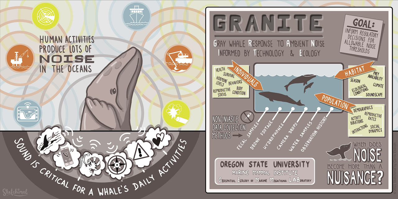
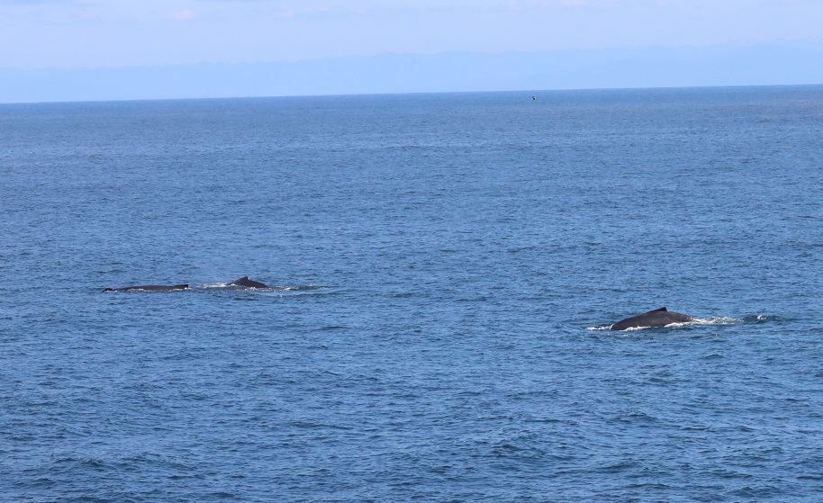
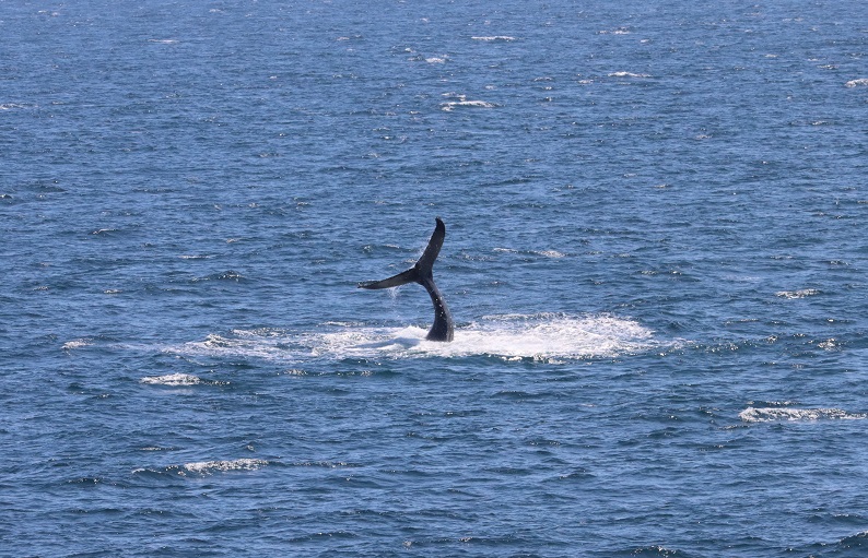
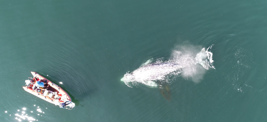
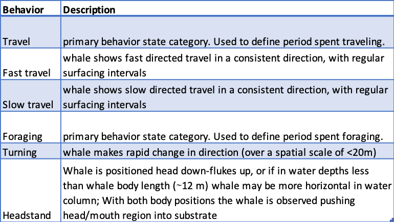
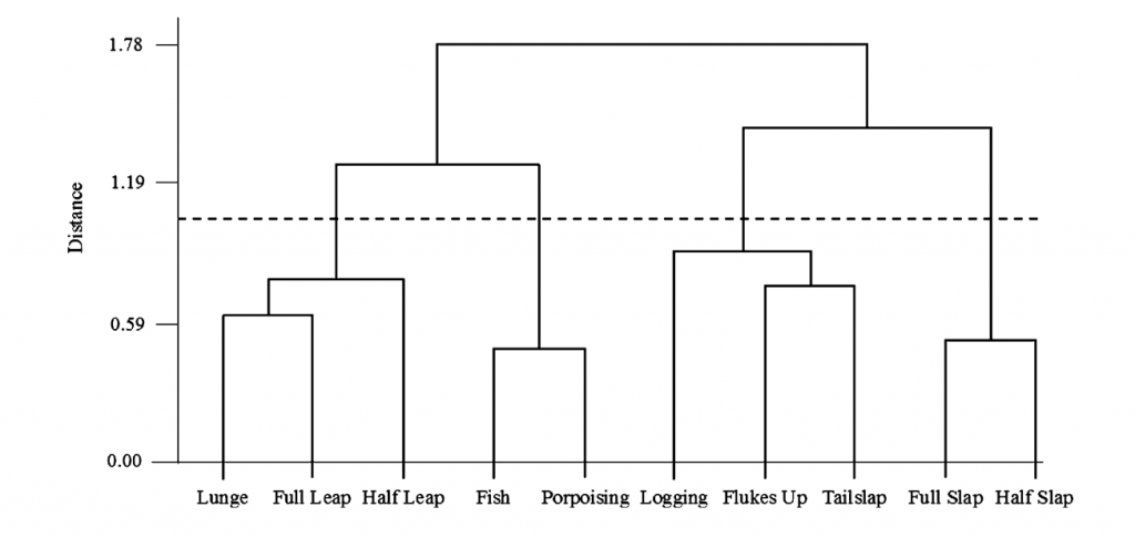
For those unfamiliar with the GRANITE project, this multifaceted and non-invasive research project evaluates how gray whales respond to chronic ambient and acute noise to inform regulatory decisions on noise thresholds (Figure 1). This project generates considerable data, often stored in separate Excel files. While this doesn’t immediately cause an issue, ongoing research projects like GRANITE and other long-term monitoring programs often need to refer to this data. Still, when scattered into separate long Excel files, it can make certain forms of analysis difficult and time-consuming. It requires considerable attention to detail, persistence, and acceptance of monotony. Today’s blog will dive into the not-so-glamorous side of science…data management and standardization!

Figure 1. Infographic for the GRANITE project. Credit: Carrie Ekeroth

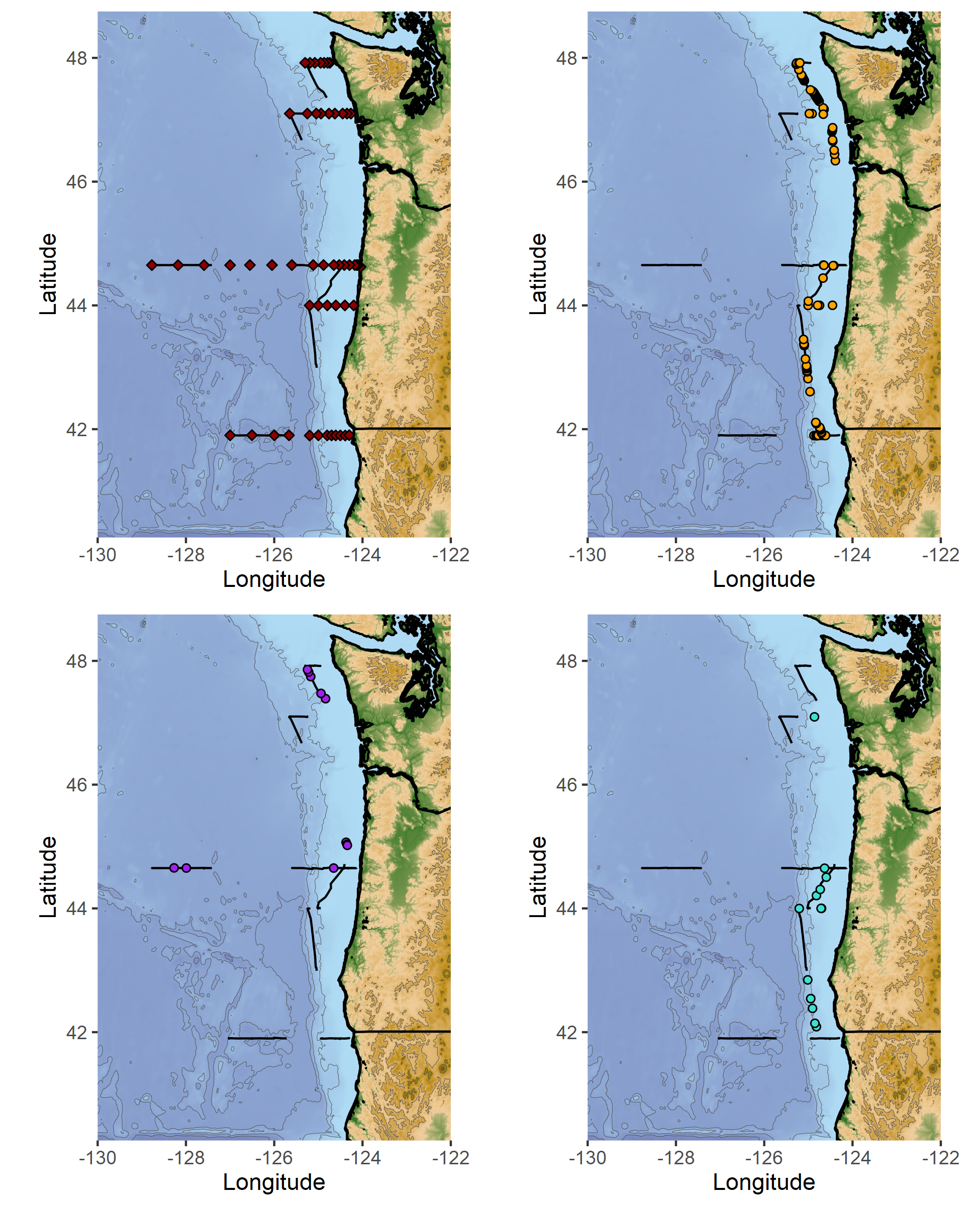
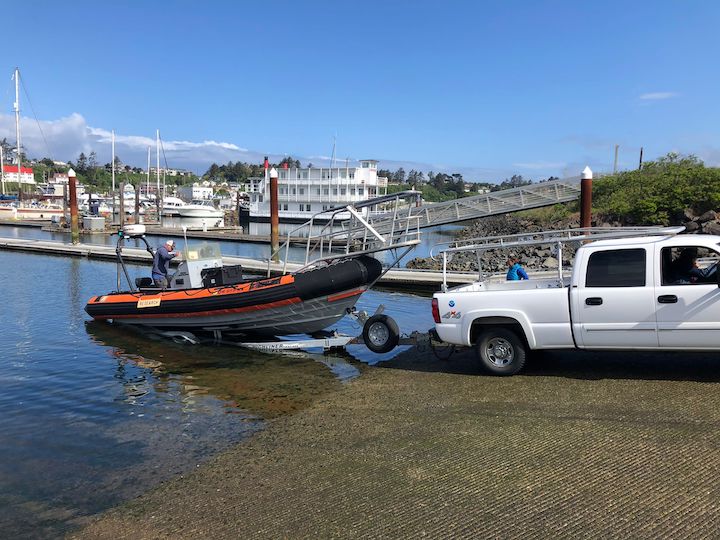
Of the plethora of data collected from the GRANITE project, I work with the GPS trackline data from the R/V Ruby, environmental data recorded on the boat, gray whale sightings data, and survey summaries for each field day. These come to me as individual yearly spreadsheets, ranging from thirty entries to several thousand. The first goal with this data is to create a standardized survey effort conditions table. The second goal is to determine the survey distance from the trackline, using the visibility for each segment, and calculate the actual area surveyed for the segment and day. This blog doesn’t go into how the area is calculated. Still, all these steps are the foundation for finding that information so the survey area can be calculated.

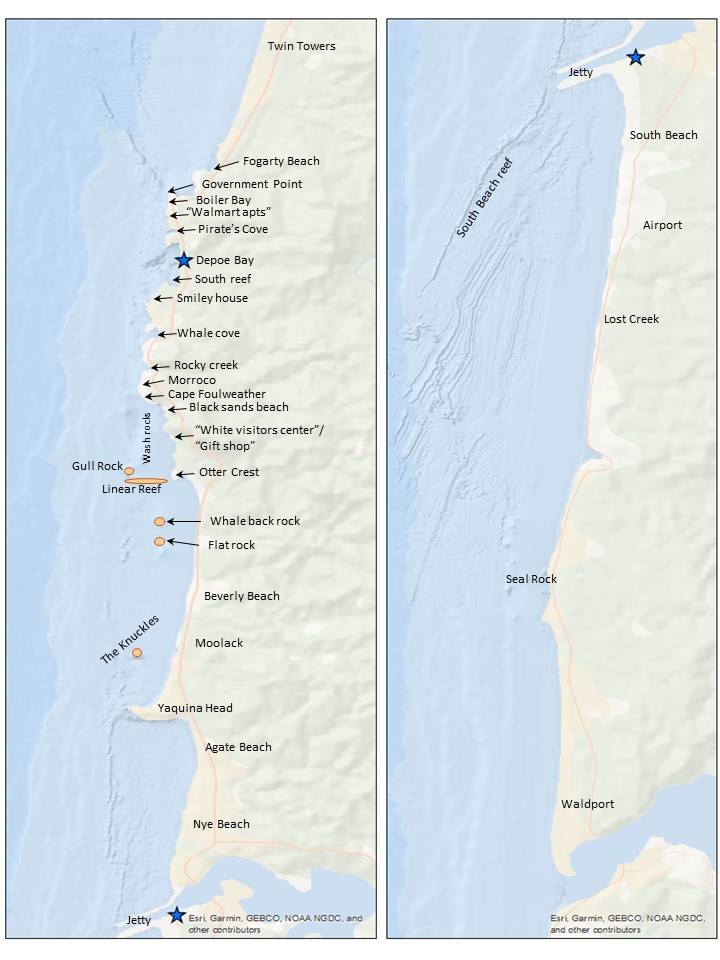
The first step requires a quick run-through of the sighting data to ensure all dates are within the designated survey area by examining the sighting code. After the date is a three-letter code representing a different starting location for the survey, such as npo for Newport and dep for Depoe Bay. If any code doesn’t match the designated codes for the survey extent, those are hidden, so they are not used in the new table. From there, filling in the table begins (Figure 2).

Figure 2. A blank survey effort conditions table with each category listed at the top in bold.

Segments for each survey day were determined based on when the trackline data changed from transit to the sighting code (i.e., 190829_1 for August 29^th, 2019, sighting 1). Transit indicated the research vessel was traveling along the coast, and crew members were surveying the area for whales. Each survey day’s GPS trackline and segment information were copied and saved into separate Excel workbook files. A specific R code would convert those files into NAD 1983 UTM Zone 10N northing and easting coordinates.

Those segments are uploaded into an ArcGIS database and mapped using the same UTM projection. The northing and easting points are imported into ArcGIS Pro as XY tables. Using various geoprocessing and editing tools, each segmented trackline for the day is created, and each line is split wherever there was trackline overlap or U shape in the trackline that causes the observation area to overlap. This splitting ensures the visibility buffer accounts for the overlap (Figure 3).

Figure 3. Segment 3 from 7/22/2019 with the visibility of 3 km portrayed as buffers. There are more than one because the trackline was split to account for the overlapping of the survey area. This approach accounts for the fact that this area where all three buffers overlap was surveyed 3 times.

Once the segment lines are created in ArcGIS, the survey area map (Figure 4) is used alongside the ArcGIS display to determine the start and end locations. An essential part of the standardization process is using the annotated locations in Figure 4 instead of the names on the basemap for the location start and endpoints. This consistency with the survey area map is both for tracking the locations through time and for the crew on the research vessel to recognize the locations. The step assists with interpreting the survey notes for conditions at the different segments. The time starts and ends, and the latitude and longitude start and end are taken from the trackline data.

Figure 4. Map of the survey area with annotated locations (Created by L. Torres, GEMM Lab)

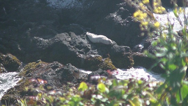
The sighting data includes the number of whales sighted, Beaufort Sea State, and swell height for the locations where whales were spotted. The environmental data from the sighting data is used as a guide when filling in the rest of the values along the trackline. When data, such as wind speed, swell height, or survey condition, is not explicitly given, matrices have been developed in collaboration with Dr. Leigh Torres to fill in the gaps in the data. These matrices and protocols for filling in the final conditions log are important tools for standardizing the environmental and condition data.

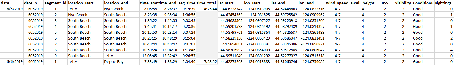
The final product for the survey conditions table is the output of all the code and matrices (Figure 5). The creation of this table will allow for accurate calculation of survey effort on each day, month, and year of the GRANITE project. This effort data is critical to evaluate trends in whale distribution, habitat use, and exposure to disturbances or threats.

Figure 5. A snippet of the completed 2019 season effort condition log.

The process of completing the table can be a very monotonous task, and there are several chances for the data to get misplaced or missed entirely. Attention to detail is a critical aspect of this project. Standardizing the GRANITE data is essential because it allows for consistency over the years and across platforms. In describing this aspect of my project, I mentioned three different computer programs using the same data. This behind-the-scenes work of creating and maintaining data standardization is critical for all projects, especially long-term research such as the GRANITE project.

Did you enjoy this blog? Want to learn more about marine life, research, and conservation? Subscribe to our blog and get a weekly message when we post a new blog. Just add your name and email into the subscribe box below.

The early phases of studying harbor seal pup behavior along the Oregon coast

By Miranda Mayhall, Masters Student, OSU Department of Fisheries, Wildlife, and Conservation Sciences, Geospatial Ecology of Marine Megafauna Lab

Recently, when expected to choose a wildlife species for behavioral observation for one of my Oregon State University graduate courses, I immediately chose harbor seals as my focus. Harbor seals (Fig 1) are an abundant species and in proximity to the Hatfield Marine Science Center (HMSC) (Steingass et al., 2019) where I will be spending much of my time this summer, making logistics easy. Studying pinnipeds (marine mammals with a finned foot, seals, walrus, and sea lions) is appealing due to their undeniably cute physique, floppy nature on land, and super agile nature in the water. I am working to iron out my methods for this study, which I hope to work through in this initial phase of my research project.

Figure 1. Harbor seal hauling out to rest on rocks off Oregon Coast near HMSC.

Behaviors:

At times it can appear that the most interesting harbor seal behaviors occur under water, and the haul out time is simply time for resting. During mating season, most adult seal behaviors take place in the water, such as the incredible vocal acoustics displayed by the males to attract the females (Matthews et al., 2018). However, I hypothesize that young pups can capitalize on haul out time by practicing becoming adults (while the adults are taking that time to rest) and therefore I plan to observe their haul out behaviors in their first summer of life. Specifically, I will document seal pup vocal behavior to evaluate how they are learning to use sound. I am beginning this study in late July, which is just after pupping season (Granquist et al., 2016). This should give me the opportunity to find pups along the Oregon coast near HMSC, so I intend to visit several locations where harbor seals are known to frequently haul out. Knowing that field work and animal behavior is unpredictable, there is no telling what behaviors I will observe on a given day, or if I will see seals at all. Some days I could come home with lots of seal data and great photos, and other days I could come home with little to report. This will be my first hurdle combined with my time limit (strictly completing this observation in the next five weeks). I intend to schedule at least eight hours of field observation at haul-out sites over the next two weeks and will adjust my schedule based on my success in data collection at that point.

Figure 2. Harbor Seals hauling out on rocks not too far from HMSC.

Timing:

Prior knowledge on harbor seal haul-out sites along the Oregon coast is clearly important for this project’s success, but I must also pay close attention to the tide cycles. During low tides, haul out locations are exposed and occupied by seals. When the tide is high, the seals are less likely to haul-out (Patterson et al., 2008). Furthermore, according to a recent study conducted on harbor seals residing on the Oregon coast, these seals spend on average 71% of their time in the water and will haul-out for the remainder of their time (Steingass et al., 2019). Therefore, it is crucial to maximize my observation time of hauled out pups wisely.

Concerning timing, I also need to observe locations and periods without too many tourists who can get near the haul-out site. As I learned recently, when children show up and start throwing rocks into the water near where harbor seals are swimming, the seals will recede from the area and no longer be available for observation. As an experiment, I waited for the noisy crowds with unchecked children to leave and only myself, my trusty sidekick (my daughter), and one quiet photographer were left on the beach. Once that happened, we noticed more and more seal heads popping up out of the water. Then they came closer and closer to the beach, splashing around doing somersaults visibly on the surface of the water. It was quite a show. I will either need to account for the presence of humans when evaluating seal behavior or assess only periods without disturbance. Seal pups are easily disturbed by humans, so I will keep a non-invasive distance while positioning myself to hear the vocals.

Figure 3. Hauled-out adult harbor seal on the Oregon coast near HMSC.

Data Collection and Analysis Approach:

The aspect of this project I am still working out is how to quantify pup vocalizations and their associated behaviors. As I mentioned, I will go out each week for eight hours and record each time I notice a pup exhibiting vocal behavior. I will categorize and describe the sound produced by the pup, and document any associated behavior of the pup or behavioral responses from nearby adult seals. Prior research has found that harbor seals are much attuned to vocal behavior. Mother harbor seals learn to quickly distinguish their own pup’s call within a few days of their birth (Sauve et al. 2015). I hypothesize that pups themselves can discern and use vocalizations, and I am excited to watch them develop over the course of my field observations.

Figure 4. Seal pup on the far-left rock, watching the adults as they appear to rest.

References

Granquist, S.M., & Hauksson, E. (2016). Seasonal, meteorological, tidal, and diurnal effects on haul-out patterns of harbour seals (Phoca vitulina) in Iceland. Polar Biology, 39 (12), 2347-2359.

Matthews, L.P., Blades, B., Parks, S. (2018). Female harbor seal (Phoca vitulina) behavioral response to playbacks of underwater male acoustic advertisement displays. PeerJ, 6, e4547.

Patterson, J., Acevedo-Gutierrez, A. (2008). Tidal influence on the haul-out behavior of harbor seals (Phoca vitulina) At all time levels. Northwestern Naturalist, 89 (1), 17-23.

Sauve, C., Beauplet, G., Hammil, M., Charrier, I. (2015). Mother-pup vocal recognition in harbour seals: influence of maternal behavior, pup voice and habitat sound properties. Animal Behavior, 105 (July 2015), 109-120

Steingass, S., Horning, M., Bishop, A. (2019). Space use of Pacific harbor seals (Phoca vitulina richardii) from two haulout locations along the Oregon coast. PloS one. 14 (7), e0219484.

Roger that, we are currently enamored

Blog by Rachel Kaplan, PhD student, Oregon State University College of Earth, Ocean, and Atmospheric Sciences and Department of Fisheries, Wildlife, and Conservation Sciences, Geospatial Ecology of Marine Megafauna Lab

Figures by Dawn Barlow, PhD Candidate, OSU Department of Fisheries, Wildlife, and Conservation Sciences, Geospatial Ecology of Marine Megafauna Lab

Hello from the RV Bell M. Shimada! We are currently sampling at an inshore station on the Heceta Head Line, which begins just south of Newport and heads out 45 nautical miles west into the Pacific Ocean. We’ll spend 10 days total at sea, which have so far been full of great weather, long days of observing, and lots of whales.

*Dawn and Rachel in matching, many-layered outfits, 125 miles offshore on the flying bridge of the RV Bell M. Shimada.*

Run by NOAA, this Northern California Current (NCC) cruise takes place three times per year. It is fabulously interdisciplinary, with teams concurrently conducting research on phytoplankton, zooplankton, seabirds, and more. The GEMM Lab will use the whale survey, krill, and oceanographic data to fuel species distribution models as part of Project OPAL. I’ll be working with this data for my PhD, and it’s great to be getting to know the region, study system, and sampling processes.

I’ve been to sea a number of times and always really enjoyed it, but this is my first time as part of a marine mammal survey. The type and timing of this work is so different from the many other types of oceanographic science that take place on a typical research cruise. While everyone else is scurrying around, deploying instruments and collecting samples at a “station” (a geographic waypoint in the ocean that is sampled repeatedly over time), we – the marine mammal team – are taking a break because we can only survey when the boat is moving. While everyone else is sleeping or relaxing during a long transit between stations, we’re hard at work up on the flying bridge of the ship, scanning the horizon for animals.

Top left: marine mammal survey effort (black lines), and oceanographic sampling stations (red diamonds). Top right: humpback whale sighting locations. Bottom left: fin whale sighting locations. Bottom right: pacific white-sided dolphin sighting locations.

During each “on effort” survey period, Dawn and I cover separate quadrants of ocean, each manning either the port or starboard side. We continuously scan the horizon for signs of whale blows or bodies, alternating between our eyes and binoculars. During long transits, we work in chunks – forty minutes on effort, and twenty minutes off effort. Staring at the sea all day is surprisingly tiring, and so our breaks often involve “going to the eye spa,” which entails pulling a neck gaiter or hat over your eyes and basking in the darkness.

Dawn has been joining these NCC cruises for the last four years, and her wealth of knowledge has been a great resource as I learn how to survey and identify marine mammals. Beyond learning the telltale signs of separate species, one of the biggest challenges has been learning how to read the sea better, to judge the difference between a frothy whitecap and a whale blow, or a distant dark wavelet and a dorsal fin. Other times, when conditions are amazing and it feels like we’re surrounded by whales, the trick is to try to predict the positions and trajectory of each whale so we don’t double-count them.

Over the last week, all our scanning has been amply rewarded. We’ve seen pods of dolphins play in our wake, and spotted Dall’s porpoises bounding alongside the ship. Here on the Heceta Line, we’ve seen a diversity of pinnipeds, including Northern fur seals, Stellar sea lions, and California sea lions. We’ve been surprised by several groups of fin whales, farther offshore than expected, and traveled alongside a pod of about 12 orcas for several minutes, which is exactly as magical as it sounds.

*Killer whales traveling alongside the Bell M. Shimada, putting on a show for the NCC science team and ship crew. Photo by Dawn Barlow.*

Notably, we’ve also seen dozens of humpbacks, including along what Dawn termed “the humpback highway” during our transit offshore of southern Oregon. One humpback put on a huge show just 200 meters from the ship, demonstrating fluke slapping behavior for several minutes. We wanted to be sure that everyone onboard could see the spectacle, so we radioed the news to the bridge, where the officers control the ship. They responded with my new favorite radio call ever: “Roger that, we are currently enamored.”

*A group of humpbacks traveling along the humpback highway. Photo by Dawn Barlow.*

*A humpback whale fluke slapping. Photo by Dawn Barlow.*

Even with long days and tired eyes, we are still constantly enamored as well. It has been such a rewarding cruise so far, and it’s hard to think of returning back to “real life” next week. For now, we’re wishing you the same things we’re enjoying – great weather, unlimited coffee, and lots of whales!

Species	Number of sightings	Total number observed
California Sea Lion	2	6
Dall’s Porpoise	3	25
Fin Whale	11	18
Humpback Whale	140	218
Killer Whale	3	21
Northern Fur Seal	9	9
Northern Right Whale Dolphin	2	8
Pacific White-sided Dolphin	13	145
Steller Sea Lion	3	3
Unidentified Baleen Whale	104	127
Unidentified Dolphin	6	28
Unidentified Whale	2	2

The learning curve never stops as the GRANITE project begins its seventh field season

Clara Bird, PhD Student, OSU Department of Fisheries, Wildlife, and Conservation Sciences, Geospatial Ecology of Marine Megafauna Lab

When I thought about what doing fieldwork would be like, before having done it myself, I imagined that it would be a challenging, but rewarding and fun experience (which it is). However, I underestimated both ends of the spectrum. I simultaneously did not expect just how hard it would be and could not imagine the thrill of working so close to whales in a beautiful place. One part that I really did not consider was the pre-season phase. Before we actually get out on the boats, we spend months preparing for the work. This prep work involves buying gear, revising and developing protocols, hiring new people, equipment maintenance and testing, and training new skills. Regardless of how many successful seasons came before a project, there are always new tasks and challenges in the preparation phase.

For example, as the GEMM Lab GRANITE project team geared up for its seventh field season, we had a few new components to prepare for. Just to remind you, the GRANITE (Gray whale Response to Ambient Noise Informed by Technology and Ecology) project’s field season typically takes place from June to mid-October of each year. Throughout this time period the field team goes out on a small RHIB (rigid hull inflatable boat), whenever the weather is good enough, to collect photo-ID data, fecal samples, and drone imagery of the Pacific Coast Feeding Group (PCFG) gray whales foraging near Newport, OR, USA. We use the data to assess the health, ecology and population dynamics of these whales, with our ultimate goal being to understand the effect of ambient noise on the population. As previous blogs have described, a typical field day involves long hours on the water looking for whales and collecting data. This year, one of our exciting new updates is that we are going out on two boats for the first part of the field season and starting our season 10 days early (our first day was May 20^th). These updates are happening because a National Science Foundation funded seismic survey is being conducted within our study area starting in June. The aim of this survey is to assess geophysical structures but provides us with an opportunity to assess the effect of seismic noise on our study group by collecting data before, during, and after the survey. So, we started our season early in order to capture the “before seismic survey” data and we are using a two-boat approach to maximize our data collection ability.

While this is a cool opportunistic project, implementing the two-boat approach came with a new set of challenges. We had to find a second boat to use, buy a new set of gear for the second boat, figure out the best way to set up our gear on a boat we had not used before, and update our data processing protocols to include data collected from two boats on the same day. Using two boats also means that everyone on the core field team works every day. This core team includes Leigh (lab director/fearless leader), Todd (research assistant), Lisa (PhD student), Ale (new post-doc), and me (Clara, PhD student). Leigh and Todd are our experts in boat driving and working with whales, Todd is our experienced drone pilot, I am our newly certified drone pilot, and Lisa, Ale, and myself are boat drivers. Something I am particularly excited about this season is that Lisa, Ale, and I all have at least one field season under our belts, which means that we get to become more involved in the process. We are learning how to trailer and drive the boats, fly the drones, and handling more of the post-field work data processing. We are becoming more involved in every step of a field day from start to finish, and while it means taking on more responsibility, it feels really exciting. Throughout most of graduate school, we grow as researchers as we develop our analytical and writing skills. But it’s just as valuable to build our skillset for field work. The ocean conditions were not ideal on the first day of the field season, so we spent our first day practicing our field skills.

For our “dry run” of a field day, we went through the process of a typical day, which mostly involved a lot of learning from Leigh and Todd. Lisa practiced her trailering and launching of the boat (figure 1), Ale and Lisa practiced driving the boat, and I practiced flying the drone (figure 2). Even though we never left the bay or saw any whales, I thoroughly enjoyed our dry run. It was useful to run through our routine, without rushing, to get all the kinks out, and it also felt wonderful to be learning in a supportive environment. Practicing new skills is stressful to say the least, especially when there is expensive equipment involved, and no one wants to mess up when they’re being watched. But our group was full of support and appreciation for the challenges of learning. We cheered for successful boat launchings and dockings, and drone landings. I left that day feeling good about practicing and improving my drone piloting skills, full of gratitude for our team and excited for the season ahead.

Figure 1. Lisa (driving the truck) launching the boat.

Figure 2. Clara (seated, wearing a black jacket) landing the drone in Ale’s hands.

All the diligent prep work paid off on Saturday with a great first day (figure 3). We conducted five GoPro drops (figure 4), collected seven fecal samples from four different whales (figure 5), and flew four drone flights over three individuals including our star from last season, Sole. Combined, we collected two trifectas (photo-ID images, fecal samples, and drone footage)! Our goal is to get as many trifectas as possible because we use them to study the relationship between the drone data (body condition and behavior) and the fecal sample data (hormones). We were all exhausted after 10 hours on the water, but we were all very excited to kick-start our field season with a great day.

Figure 3. Lisa on the bow pulpit during our first sighting of the day.

Figure 4. Lisa doing a GoPro drop, she’s lowering the GoPro into the water using the line in her hands.

Figure 5. Clara and Ale collecting a fecal sample.

On Sunday, just one boat went out to collect more data from Sole after a rainy morning and I successfully flew over her from launching to landing! We have a long season ahead, but I am excited to learn and see what data we collect. Stay tuned for more updates from team GRANITE as our season progresses!

From land, sea,… and space: searching for whales in the vast ocean

By Solène Derville, Postdoc, OSU Department of Fisheries, Wildlife, and Conservation Science, Geospatial Ecology of Marine Megafauna Lab

The ocean is vast.

What I mean is that the vastness of the ocean is very hard to mentally visualize. When facing a conservation issue such as increased whale entanglement along the US West Coast (see OPAL project ), a tempting solution may be to suggest « let’s go see where the whales are and report their location to the fishermen?! ». But, it only takes a little calculation to realize how impractical this idea is.

Let’s roll out the numbers. The US West Coast exclusive economic zone (EEZ) stretches from the coast out to 200 nautical miles offshore, as prescribed by the 1982 United Nations Convention on the Law of the Sea. It covers an area of 825,549 km² (Figure 1). Now, imagine that you wish to survey this area for marine mammals. Using a vessel such as the R/V Bell M. Shimada that is used for the Northern California Current Ecosystem surveys cruises (NCC cruises, see Dawn and Rachel’s last blog), we may detect whales at a distance of roughly 6 km (based on my preliminary results). This distance of detection depends on the height of the observer, hence the height of the flying bridge where she/he is standing (the observer’s height may also be accounted for, but unless she/he is a professional basket-ball player, I think it can be neglected here). The Shimada is quite a large ship and it’s flying bridge is 13 meters above the water. Two observers may survey the water on each side of the trackline.

Considering that the vessel is moving at 8 knots (~15 km/h), we may expect to be effectively surveying 180 km² per hour (6x2x15). That’s not too bad, right?

Again, perspective is the key. If we divide the West Coast EEZ surface by 180 km² we can estimate that it would take 2,752 hours to survey this entire region. With an average of 12 hours of daylight, this takes us to…

382 DAYS OF SURVEY, searching for marine mammals over the US West Coast. Considering that observations cannot be undertaken on days with bad weather (fog, heavy rain, strong winds…), it might take more than a year and a half to complete the survey! And what would the marine mammals have done in the meantime? Move…

This little math exercise proves that exhaustively searching for the needle in the haystack from a vessel is not the way to go if we are to describe whale distribution and help mitigate the risk of entanglement. And using another platform of observation is not necessarily the solution. The OPAL project has relied on a great collaboration with the United States Coast Guard to survey Oregon waters. The USCG helicopters travel fast compared to a vessel, about 90 knots (167 km/h). As a result, more ground is covered but the speed at which it is traveling prevents the observer from detecting whales that are very far away. Based on the last analysis I ran for the OPAL project, whales are usually detected up to 3 km from the helicopter (only 5 % of sightings exceed that distance). In addition, the helicopter generally only has capacity for one observer at a time.

If we replicate the survey time calculation from above for the USCG helicopter, we realize that even with a fast-moving aerial survey platform it would still take 137 days to cover the West Coast EEZ.

**Figure 1**. What is the best survey method to document marine mammal occurrence in the US West Coast Exclusive Economic zone (EEZ)?

First, we can model and extrapolate. This approach is the path we are taking with the OPAL project: we survey Oregon waters in 4 different areas along the coast each month, then model observed whale densities as a function of topographic and oceanographic variables, and then predict whale probability of presence over the entire region. These predictions are based on the assumption that our survey design effectively sampled the variety of environmental conditions experienced by whales over the study region, which it certainly did considering that all sites are surveyed year-round.

An alternative approach that has been recently discussed in the GEMM Llab, is the use of satellite images to detect whales along the coast. A communication entitled « The Potential of Satellite Imagery for Surveying Whales » was published last month in the Sensors Journal (Höschle et al., 2021) and presents the opportunities offered by this relatively new technology. The WorldView-3 satellite, owned by the company Digitalglobe and launched in 2016, has made it possible to commercialize imagery with a resolution never reached before, of the order of 30 cm per pixel. These very high resolution (VHR) satellite images make it possible to identify several species of large whales (Cubaynes et al. al., 2019) and to estimate their density (Bamford et al., 2020). Furthermore, machine learning algorithms, such as Neural Networks, have proved quite efficient at automatically detecting whales in satellite images (Guirado et al., 2019, Figure 2). While several new ultra-high resolution imaging satellites are expected to be launched in 2021 (by Maxar Technologies and Airbus), this “remote” approach looks like a promising avenue to detect whales over vast regions while drinking a cup of coffee at the office.

**Figure 2.** Illustration of a whale detection algorithm working on a gridded satellite image (DigitalGlobe). Source: Guirado et al., 2019.

But like any other data collection method, satellites have their drawbacks. We recently discovered that these VHR satellites are routinely switched off while passing above the ocean. Specific inquiries would need to be made to acquire data over our study areas, which would be at great expense. One of the cheapest provider I found is the Soar platform, that provides images at 50 cm resolution in partnership with the Chinese Aerospace Science and Technology Corporation. They advertise daily images anywhere on earth at $10 USD per km². This might sound cheap at first glance, but circling back to our US West Coast EEZ area calculations, we estimate that surveying this region entirely with satellite imagery would cost more than $8 million USD.

Yet, we have to look forward. The use of satellite imagery is likely to broaden and increase in the coming years, with a possible decrease in cost. Quoting Höschle et al. (2021) ‘To protect our world’s oceans, we need a global effort and we need to create opportunities for that to happen’.

Will satellites soon save whales?

References

Bamford, C. C. G. et al. A comparison of baleen whale density estimates derived from overlapping satellite imagery and a shipborne survey. Sci. Rep. 10, 1–12 (2020).

Cubaynes, H. C., Fretwell, P. T., Bamford, C., Gerrish, L. & Jackson, J. A. Whales from space: Four mysticete species described using new VHR satellite imagery. Mar. Mammal Sci. 35, 466–491 (2019).

Guirado, E., Tabik, S., Rivas, M. L., Alcaraz-Segura, D. & Herrera, F. Whale counting in satellite and aerial images with deep learning. Sci. Rep. 9, 1–12 (2019).

Höschle, C., Cubaynes, H. C., Clarke, P. J., Humphries, G. & Borowicz, A. The potential of satellite imagery for surveying whales. Sensors 21, 1–6 (2021).

Lessons learned from (not) going to sea

By Rachel Kaplan¹ and Dawn Barlow²

¹PhD student, Oregon State University College of Earth, Ocean, and Atmospheric Sciences and Department of Fisheries and Wildlife, Geospatial Ecology of Marine Megafauna Lab

²PhD Candidate, Oregon State University Department of Fisheries and Wildlife, Geospatial Ecology of Marine Megafauna Lab

“Hurry up and wait.” A familiar phrase to anyone who has conducted field research. A flurry of preparations, followed by a waiting game—waiting for the weather, waiting for the right conditions, waiting for unforeseen hiccups to be resolved. We do our best to minimize unknowns and unexpected challenges, but there is always uncertainty associated with any endeavor to collect data at sea. We cannot control the whims of the ocean; only respond as best we can.

On 15 February 2021, we were scheduled to board the NOAA Ship Bell M. Shimada as marine mammal observers for the Northern California Current (NCC) ecosystem survey, a recurring research cruise that takes place several times each year. The GEMM Lab has participated in this multidisciplinary data collection effort since 2018, and we are amassing a rich dataset of marine mammal distribution in the region that is incorporated into the OPAL project. February is the middle of wintertime in the North Pacific, making survey conditions challenging. For an illustration of this, look no further than at the distribution of sightings made during the February 2018 cruise (Fig. 1), when rough sea conditions meant only a few whales were spotted.

**Figure 1.** (A) Map of marine mammal survey effort (gray tracklines) and baleen whale sightings recorded onboard the NOAA ship R/V Shimada during each of the NCC research cruises to-date and (B) number of individuals sighted per cruise since 2018. Note the amount of survey effort conducted in February 2018 (top left panel) compared to the very low number of whales sighted. Data summary and figures courtesy of Solene Derville.

Now, this is February 2021 and the world is still in the midst of navigating the global coronavirus pandemic that has affected every aspect of our lives. The September 2020 NCC cruise was the first NOAA fisheries cruise to set sail since the pandemic began, and all scientists and crew followed a strict shelter-in-place protocol among other COVID risk mitigation measures. Similarly, we sheltered in place in preparation for the February 2021 cruise. But here’s where the weather comes in yet again. Not only did we have to worry about winter weather at sea, but the inclement conditions across the country meant our COVID tests were delayed in transit—and we could not board the ship until everyone tested negative. By the time our results were in, the marine forecast was foreboding, and the Captain determined that the weather window for our planned return to port had closed.

So, we are still on shore. The ship never left the dock, and NCC February 2021 will go on the record as “NAs” rather than sightings of marine mammal presence or absence. So it goes. We can dedicate all our energy to studying the ocean and these spectacularly dynamic systems, but we cannot control them. It is an important and humbling reminder. But as we have continued to learn over the past year, there are always silver linings to be found.

Even though we never made it to the ship, it turns out there’s a lot you can get done onshore. Dawn has sailed on several NCC cruises before, and one of the goals this time was to train Rachel for her first stint at marine mammal survey work. This began at Dawn’s house in Newport, where we sheltered in place together for the week prior to our departure date.

We walked through the iPad program we use to enter data, looked through field guides, and talked over how to respond in different scenarios we might encounter while surveying for marine mammals at sea. We also joined Solene, a postdoc working on the OPAL project, for a Zoom meeting to edit the distance sampling protocol document. It was great training to discuss the finer points of data collection together, with respect to how that data will ultimately be worked into our species distribution models.

The February NCC cruise is famously rough, and a tough time to sight whales (Fig. 1). This low sighting rate arises from a combination of factors: baleen whales typically spend the winter months on their breeding grounds in lower latitudes so their density in Oregon waters is lower, and the notorious winter sea state makes sighting conditions difficult. Solene signed off our Zoom call with, “Go collect that high-quality absence data, girls!” It was a good reminder that not seeing whales is just as important scientifically as seeing them—though sometimes, of course, it’s not possible to even get out where you can’t see them. Furthermore, all absence data is not created equal. The quality of the absence data we can collect deteriorates along with the weather conditions. When we ultimately use these survey data to fuel species distribution models, it’s important to account for our confidence in the periods with no whale sightings.

In addition to the training we were able to conduct on land, the biggest silver lining came just from sheltering in place together. We had only met over Zoom previously, and spending this time together gave us the opportunity to get to know each other in real life and become friends. The week involved a lot of fabulous cooking, rainy walks, and an ungodly number of peanut butter cups. Even though the cruise couldn’t happen, it was such a rich week. The NCC cruises take place several times each year, and the next one is scheduled for May 2021. We’ll keep our fingers crossed for fair winds and negative COVID tests in May!

**Figure 2.** Dawn’s dog Quin was a great shelter in place buddy. She was not sad that the cruise was canceled.

Marine mammals of the Northern California Current, 2020 edition

By Dawn Barlow, PhD student, OSU Department of Fisheries and Wildlife, Geospatial Ecology of Marine Megafauna Lab

Clara and I have just returned from ten fruitful days at sea aboard NOAA Ship Bell M. Shimada as part of the Northern California Current (NCC) ecosystem survey. We surveyed between Crescent City, California and La Push, Washington, collecting data on oceanography, phytoplankton, zooplankton, and marine mammals (Fig. 1). This year represents the third year I have participated in these NCC cruises, which I have come to cherish. I have become increasingly confident in my marine mammal observation and species identification skills, and I have become more accepting of the things out of my control – the weather, the sea state, the many sightings of “unidentified whale species”. Careful planning and preparation are critical, and yet out at sea we are ultimately at the whim of the powerful Pacific Ocean. Another aspect of the NCC cruises that I treasure is the time spent with members of the science team from other disciplines. The chatter about water column features, musings about plankton species composition, and discussions about what drives marine mammal distribution present lively learning opportunities throughout the cruise. Our concurrent data collection efforts and ongoing conversations allow us to piece together a comprehensive picture of this dynamic NCC ecosystem, and foster a collaborative research environment.

**Figure 1.** Data collection effort for the NCC September 2020 cruise, between Crescent City, CA, and La Push, WA. Red points represent oceanographic sampling stations, and black lines show the track of the research vessel during marine mammal survey effort.

Every time I head to sea, I am reminded of the patchy distribution of resources in the vast and dynamic marine environment. On this recent cruise we documented a stark contrast between expansive stretches of warm, blue, stratified, and seemingly empty ocean and areas that were plankton-rich and supported multi-species feeding frenzies that had marine mammal observers like me scrambling to keep track of everything. This year, we were greeted by dozens of blue and humpback whales in the productive waters off Newport, Oregon. Off Crescent City, California, the water was very warm, the plankton community was dominated by gelatinous species like pyrosomes, salps, and other jellies, and the marine mammals were virtually absent except for a few groups of common dolphins. To the north, the plume of water flowing from the Columbia River created a front between water masses, where we found ourselves in the midst of pacific white-sided dolphins, northern right whale dolphins, and humpback whales. These observations highlight the strength of ecosystem-scale and multi-disciplinary data collection efforts such as the NCC surveys. By drawing together information on physical oceanography, primary productivity, zooplankton community composition and abundance, and marine predator distribution, we can gain a nearly comprehensive picture of the dynamics within the NCC over a broad spatial scale.

This year, the marine mammals delivered and kept us observers busy. We lucked out with good survey conditions and observed many different species throughout the NCC (Table 1, Fig. 2).

Table 1. Summary of all marine mammal sightings from the NCC September 2020 cruise.

**Figure 2.** Maps showing kernel densities of four frequently observed and widely distributed species seen during the cruise. Black lines show the track of the research vessel during marine mammal survey effort, white points represent sighting locations, and colors show kernel density estimates weighted by group size at each sighting.

This year’s NCC cruise was unique. We went to sea as a global pandemic, wildfires, and political tensions continue to strain this country and our communities. This cruise was the first NOAA Fisheries cruise to set sail since the start of the pandemic. Our team of scientists and the ship’s crew went to great lengths to make it possible, including a seven-day shelter-in-place period and COVID-19 tests prior to cruise departure. As a result of these extra challenges and preparations, I think we were all especially grateful to be on the water, collecting data. At-sea fieldwork is always challenging, but morale was up, spirits were high, and laughs were frequent despite smiles being concealed by our masks. I am grateful for the opportunity to participate in this ongoing valuable data collection effort, and to be part of this team. Thanks to all who made it such a memorable cruise.

**Figure 3.** The NCC September 2020 science team at the end of a successful research cruise! Fieldwork in the time of COVID-19 presents many logistical challenges, but this team rose to the occasion and completed a safe and fruitful survey despite the circumstances.

How we plan to follow whales

Clara Bird, Masters Student, OSU Department of Fisheries and Wildlife, Geospatial Ecology of Marine Megafauna Lab

The GEMM Lab gray whale team is in the midst of preparing for our fifth field season studying the Pacific Coast Foraging Group (PCFG): whales that forage off the coast of Newport, OR, USA each summer. On any given good weather day from June to October, our team is out on the water in a small zodiac looking for gray whales (Figure 1). When we find a gray whale, we try to collect photo ID data, fecal samples, drone data, and behavioral data. We use the drone data to study both the whale’s body condition and their behavior. In a previous blog, I described ethograms and how I would like to use the behavior data from drone videos to classify behaviors, with the ultimate goal of understanding how gray whale behavior varies across space, time, and by individual. However, this explanation of studying whale behavior is actually a bit incomplete. Before we start fieldwork, we first need to decide how to collect that data.

Figure 1. Image of GEMM lab team collecting gray whale UAS data. Image taken under NOAA/NMFS permit #16111

As observers, we are far from omnipresent and there is no way to know what the animals are doing all of the time. In any environment, scientists have to decide when and where to observe their animals and what behaviors they are interested in recording. In many studies, behavior is recorded live by an observer. In those studies, other limitations need to be taken into account, such as human error and observer fatigue. Collecting behavioral data is particularly challenging in the marine environment. Cetaceans spend most of their lives out of sight from humans, their time at the surface is brief, and when they appear together in large groups it can be very difficult to keep track of who is doing what when. Imagine being in a boat trying to keep track of what three different whales are doing without a pre-determined method – the task could quickly become overwhelming and biased. This is why we need a methodology for collecting and classifying behavior. We cannot study behavior without acknowledging these limitations and the potential biases that come with the methods we choose. Different data collection methods are better suited to address different questions.

The use of drones gives us the ability to record cetacean behavior non-invasively, from a perspective that allows greater observation (Figure 2, Torres et al. 2018), and for later review, which is a significant improvement. However, as we prepare to collect more behavior data, we need to study the methods and understand the benefits and disadvantages of each approach so that we capture the information we need without bias. Altmann (1974) provides a thorough overview of behavioral sampling methods.

Figure 2. Diagram illustrating “whale surface time” relative to “whale visible time” data as collected from an unmanned aerial systems (UAS) aircraft flying over a gray whale as it moves sequentially (from right to left) from “headstand” foraging to surfacing. Figure from Torres et al. (2018).

Ad libitum behavioral sampling has no structure and occurs when we find a group of whales and just write down everything they are doing. This method is a good first step, however it comes with bias. Without structure, we cannot be sure that there was an equal probability of detecting each kind of behavior; this problem is called detectability bias. This type of bias is an issue if we are trying to answer questions about how often a behavior occurs, or what percent of time is spent in each behavior state. This is a bias to be especially concerned about when it comes to cetaceans because there are many examples of behaviors with different levels of detectability. An extreme example would be the detectability of breaching versus a behavior that takes place under the surface. A breaching whale is easier to spot and more exciting, which could lead to results suggesting that whales breach more often than they do relative to underwater behaviors. While it’s impossible to eliminate detectability bias, other sampling methods employ decision rules to try and reduce its effect. Many decision rules revolve around time, such as setting a minimum or maximum observation time interval. Other time rules involve recording the behavior state at set intervals of time (e.g., every 5 minutes). Setting observation boundaries helps standardize the methods and the data being collected.

In a structured sampling plan, the first big decision that needs to be addressed is the need to know the duration of behaviors. Point events do not include duration data but can be used to study the frequencies of behaviors. For example, if my research question was “Do whales perform “headstands” in a specific habitat type?”, then I would need point events of headstanding behavior. But, if I wanted to ask, “Do whales spend more time spent headstanding in a specific habitat type than in other habitat types?”, I would need headstanding to be a state event. State events are events with associated duration information and can be used for activity budgets. Activity budgets show how much time an animal spends in each behavior state. Some sampling methods focus on collecting only point events. However, to get the most complete understanding of behavior I think it’s important to collect both. Focal animal follows are another method of collecting more detailed data and is commonly used in cetacean studies.

The explanation of a focal follow method is in the name. We focus on one individual, follow it, and record all of its behaviors. When employing this method, decisions are made about how an individual is chosen and how long it is followed. In some cases, the behavior of this animal is used as a proxy for the behavior of an entire group. I essentially use the focal follow method in my research. While I review drone footage to record behavioral data instead of recording behaviors live in the field, I focus on one individual a time as I go through the videos. To do this I use a software called BORIS (Friard and Gamba 2016) to mark the time of each behavior per individual (Figure 3). If there are three individuals in a video, I’ll review the footage three times to record behaviors once per individual, focusing on each in turn.

While the drone footage brings the advantages of time to review and a better view of the whale, we are constrained by the duration of a flight. Focal follows would ideally last longer than the ~15 minutes of battery life per drone flight. Our previously collected footage gives us snapshots of behavior, and this makes it challenging to compare and analyze durations of behaviors. Therefore, I am excited that we are going to try conducting drone focal follows this summer by swapping out drones when power runs low to achieve longer periods of video coverage of whale behavior. I’ll be able to use these data to move from snapshots to analyzing longer clips and better understanding the behavioral ecology of gray whales. As exciting as this opportunity is, it also presents the challenge of method development. So, I now need to develop decision rules and data collection methods to answer the questions that I have been eagerly asking.

References

Altmann, Jeanne. 1974. “Observational Study of Behavior: Sampling Methods.” Behaviour 49 (3–4): 227–66. https://doi.org/10.1163/156853974X00534.

Friard, Olivier, and Marco Gamba. 2016. “BORIS: A Free, Versatile Open-Source Event-Logging Software for Video/Audio Coding and Live Observations.” Methods in Ecology and Evolution 7 (11): 1325–30. https://doi.org/10.1111/2041-210X.12584.

Torres, Leigh G., Sharon L. Nieukirk, Leila Lemos, and Todd E. Chandler. 2018. “Drone up! Quantifying Whale Behavior from a New Perspective Improves Observational Capacity.” Frontiers in Marine Science 5 (SEP). https://doi.org/10.3389/fmars.2018.00319.

Classifying cetacean behavior

Clara Bird, Masters Student, OSU Department of Fisheries and Wildlife, Geospatial Ecology of Marine Megafauna Lab

The GEMM lab recently completed its fourth field season studying gray whales along the Oregon coast. The 2019 field season was an especially exciting one, we collected rare footage of several interesting gray whale behaviors including GoPro footage of a gray whale feeding on the seafloor, drone footage of a gray whale breaching, and drone footage of surface feeding (check out our recently released highlight video here). For my master’s thesis, I’ll use the drone footage to analyze gray whale behavior and how it varies across space, time, and individual. But before I ask how behavior is related to other variables, I need to understand how to best classify the behaviors.

How do we collect data on behavior?

One of the most important tools in behavioral ecology is an ‘ethogram’. An ethogram is a list of defined behaviors that the researcher expects to see based on prior knowledge. It is important because it provides a standardized list of behaviors so the data can be properly analyzed. For example, without an ethogram, someone observing human behavior could say that their subject was walking on one occasion, but then say strolling on a different occasion when they actually meant walking. It is important to pre-determine how behaviors will be recorded so that data classification is consistent throughout the study. Table 1 provides a sample from the ethogram I use to analyze gray whale behavior. The specificity of the behaviors depends on how the data is collected.

Table 1. Sample from gray whale ethogram. Based on ethogram from Torres et al. (2018).

In marine mammal ecology, it is challenging to define specific behaviors because from the traditional viewpoint of a boat, we can only see what the individuals are doing at the surface. The most common method of collecting behavioral data is called a ‘focal follow’. In focal follows an individual, or group, is followed for a set period of time and its behavioral state is recorded at set intervals. For example, a researcher might decide to follow an animal for an hour and record its behavioral state at each minute (Mann 1999). In some studies, they also recorded the location of the whale at each time point. When we use drones our methods are a little different; we collect behavioral data in the form of continuous 15-minute videos of the whale. While we collect data for a shorter amount of time than a typical focal follow, we can analyze the whole video and record what the whale was doing at each second with the added benefit of being able to review the video to ensure accuracy. Additionally, from the drone’s perspective, we can see what the whales are doing below the surface, which can dramatically improve our ability to identify and describe behaviors (Torres et al. 2018).

Categorizing Behaviors

In our ethogram, the behaviors are already categorized into primary states. Primary states are the broadest behavioral states, and in my study, they are foraging, traveling, socializing, and resting. We categorize the specific behaviors we observe in the drone videos into these categories because they are associated with the function of a behavior. While our categorization is based on prior knowledge and critical evaluation, this process can still be somewhat subjective. Quantitative methods provide an objective interpretation of the behaviors that can confirm our broad categorization and provide insight into relationships between categories. These methods include path characterization, cluster analysis, and sequence analysis.

Path characterization classifies behaviors using characteristics of their track line, this method is similar to the RST method that fellow GEMM lab graduate student Lisa Hildebrand described in a recent blog. Mayo and Marx (1990) analyzed the paths of surface foraging North Atlantic Right Whales and were able to classify the paths into primary states; they found that the path of a traveling whale was more linear and then paths of foraging or socializing whales that were more convoluted (Fig 1). I plan to analyze the drone GPS track line as a proxy for the whale’s track line to help distinguish between traveling and foraging in the cases where the 15-minute snapshot does not provide enough context.

Figure 1. Figure from Mayo and Marx (1990) showing different track lines symbolized by behavior category.

Cluster analysis looks for natural groupings in behavior. For example, Hastie et al. (2004) used cluster analysis to find that there were four natural groupings of bottlenose dolphin surface behaviors (Fig. 2). I am considering using this method to see if there are natural groupings of behaviors within the foraging primary state that might relate to different prey types or habitat. This process is analogous to breaking human foraging down into sub-categories like fishing or farming by looking for different foraging behaviors that typically occur together.

Figure 2. Figure from Hastie et al. (2004) showing the results of a hierarchical cluster analysis.

Lastly, sequence analysis also looks for groupings of behaviors but, unlike cluster analysis, it also uses the order in which behaviors occur. Slooten (1994) used this method to classify Hector’s dolphin surface behaviors and found that there were five classes of behaviors and certain behaviors connected the different categories (Fig. 3). This method is interesting because if there are certain behaviors that are consistently in the same order then that indicates that the order of events is important. What function does a specific sequence of behaviors provide that the behaviors out of that order do not?

Figure 3. Figure from Slooten (1994) showing the results of sequence analysis.

Think about harvesting fruits and vegetables from a garden: the order of how things are done matters and you might use different methods to harvest different kinds of produce. Without knowing what food was being harvested, these methods could detect that there were different harvesting methods for different fruits or veggies. By then studying when and where the different methods were used and by whom, we could gain insight into the different functions and patterns associated with the different behaviors. We might be able to detect that some methods were always used in certain habitat types or that different methods were consistently used at different times of the year.

Behavior classification methods such as these described provide a more refined and detailed analysis of categories that can then be used to identify patterns of gray whale behaviors. While our ultimate goal is to understand how gray whales will be affected by a changing environment, a comprehensive understanding of their current behavior serves as a baseline for that future study.

References

Burnett, J. D., Lemos, L., Barlow, D., Wing, M. G., Chandler, T., & Torres, L. G. (2019). Estimating morphometric attributes of baleen whales with photogrammetry from small UASs: A case study with blue and gray whales. Marine Mammal Science, 35(1), 108–139. https://doi.org/10.1111/mms.12527

Darling, J. D., Keogh, K. E., & Steeves, T. E. (1998). Gray whale (Eschrichtius robustus) habitat utilization and prey species off Vancouver Island, B.C. Marine Mammal Science, 14(4), 692–720. https://doi.org/10.1111/j.1748-7692.1998.tb00757.x

Hastie, G. D., Wilson, B., Wilson, L. J., Parsons, K. M., & Thompson, P. M. (2004). Functional mechanisms underlying cetacean distribution patterns: Hotspots for bottlenose dolphins are linked to foraging. Marine Biology, 144(2), 397–403. https://doi.org/10.1007/s00227-003-1195-4

Mann, J. (1999). Behavioral sampling methods for cetaceans: A review and critique. Marine Mammal Science, 15(1), 102–122. https://doi.org/10.1111/j.1748-7692.1999.tb00784.x

Slooten, E. (1994). Behavior of Hector’s Dolphin: Classifying Behavior by Sequence Analysis. Journal of Mammalogy, 75(4), 956–964. https://doi.org/10.2307/1382477

Torres, L. G., Nieukirk, S. L., Lemos, L., & Chandler, T. E. (2018). Drone up! Quantifying whale behavior from a new perspective improves observational capacity. Frontiers in Marine Science, 5(SEP). https://doi.org/10.3389/fmars.2018.00319

Mayo, C. A., & Marx, M. K. (1990). Surface foraging behaviour of the North Atlantic right whale, Eubalaena glacialis, and associated zooplankton characteristics. Canadian Journal of Zoology, 68(10), 2214–2220. https://doi.org/10.1139/z90-308

Data Wrangling to Assess Data Availability: A Data Detective at Work

By Alexa Kownacki, Ph.D. Student, OSU Department of Fisheries and Wildlife, Geospatial Ecology of Marine Megafauna Lab

Data wrangling, in my own loose definition, is the necessary combination of both data selection and data collection. Wrangling your data requires accessing then assessing your data. Data collection is just what it sounds like: gathering all data points necessary for your project. Data selection is the process of cleaning and trimming data for final analyses; it is a whole new bag of worms that requires decision-making and critical thinking. During this process of data wrangling, I discovered there are two major avenues to obtain data: 1) you collect it, which frequently requires an exorbitant amount of time in the field, in the lab, and/or behind a computer, or 2) other people have already collected it, and through collaboration you put it to a good use (often a different use then its initial intent). The latter approach may result in the collection of so much data that you must decide which data should be included to answer your hypotheses. This process of data wrangling is the hurdle I am facing at this moment. I feel like I am a data detective.

Data wrangling illustrated by members of the R-programming community. (Image source: R-bloggers.com)

My project focuses on assessing the health conditions of the two ecotypes of bottlenose dolphins between the waters off of Ensenada, Baja California, Mexico to San Francisco, California, USA between 1981-2015. During the government shutdown, much of my data was inaccessible, seeing as it was in possession of my collaborators at federal agencies. However, now that the shutdown is over, my data is flowing in, and my questions are piling up. I can now begin to look at where these animals have been sighted over the past decades, which ecotypes have higher contaminant levels in their blubber, which animals have higher stress levels and if these are related to geospatial location, where animals are more susceptible to human disturbance, if sex plays a role in stress or contaminant load levels, which environmental variables influence stress levels and contaminant levels, and more!

Alexa, alongside collaborators, photographing transiting bottlenose dolphins along the coastline near Santa Barbara, CA in 2015 as part of the data collection process. (Image source: Nick Kellar).

Over the last two weeks, I was emailed three separate Excel spreadsheets representing three datasets, that contain partially overlapping data. If Microsoft Access is foreign to you, I would compare this dilemma to a very confusing exam question of “matching the word with the definition”, except with the words being in different languages from the definitions. If you have used Microsoft Access databases, you probably know the system of querying and matching data in different databases. Well, imagine trying to do this with Excel spreadsheets because the databases are not linked. Now you can see why I need to take a data management course and start using platforms other than Excel to manage my data.

A visual interpretation of trying to combine datasets being like matching the English definition to the Spanish translation. (Image source: Enchanted Learning)

In the first dataset, there are 6,136 sightings of Common bottlenose dolphins (Tursiops truncatus) documented in my study area. Some years have no sightings, some years have fewer than 100 sightings, and other years have over 500 sightings. In another dataset, there are 398 bottlenose dolphin biopsy samples collected between the years of 1992-2016 in a genetics database that can provide the sex of the animal. The final dataset contains records of 774 bottlenose dolphin biopsy samples collected between 1993-2018 that could be tested for hormone and/or contaminant levels. Some of these samples have identification numbers that can be matched to the other dataset. Within these cross-reference matches there are conflicting data in terms of amount of tissue remaining for analyses. Sorting these conflicts out will involve more digging from my end and additional communication with collaborators: data wrangling at its best. Circling back to what I mentioned in the beginning of this post, this data was collected by other people over decades and the collection methods were not standardized for my project. I benefit from years of data collection by other scientists and I am grateful for all of their hard work. However, now my hard work begins.

The cutest part of data wrangling: finding adorable images of bottlenose dolphins, photographed during a coastal survey. (Image source: Alexa Kownacki).

There is also a large amount of data that I downloaded from federally-maintained websites. For example, dolphin sighting data from research cruises are available for public access from the OBIS (Ocean Biogeographic Information System) Sea Map website. It boasts 5,927,551 records from 1,096 data sets containing information on 711 species with the help of 410 collaborators. This website is incredible as it allows you to search through different data criteria and then download the data in a variety of formats and contains an interactive map of the data. You can explore this at your leisure, but I want to point out the sheer amount of data. In my case, the OBIS Sea Map website is only one major platform that contains many sources of data that has already been collected, not specifically for me or my project, but will be utilized. As a follow-up to using data collected by other scientists, it is critical to give credit where credit is due. One of the benefits of using this website, is there is information about how to properly credit the collaborators when downloading data. See below for an example:

Example citation for a dataset (Dataset ID: 1201):

Lockhart, G.G., DiGiovanni Jr., R.A., DePerte, A.M. 2014. Virginia and Maryland Sea Turtle Research and Conservation Initiative Aerial Survey Sightings, May 2011 through July 2013. Downloaded from OBIS-SEAMAP (http://seamap.env.duke.edu/dataset/1201) on xxxx-xx-xx.

Citation for OBIS-SEAMAP:

Halpin, P.N., A.J. Read, E. Fujioka, B.D. Best, B. Donnelly, L.J. Hazen, C. Kot, K. Urian, E. LaBrecque, A. Dimatteo, J. Cleary, C. Good, L.B. Crowder, and K.D. Hyrenbach. 2009. OBIS-SEAMAP: The world data center for marine mammal, sea bird, and sea turtle distributions. Oceanography 22(2):104-115

Another federally-maintained data source that boasts more data than I can quantify is the well-known ERDDAP website. After a few Google searches, I finally discovered that the acronym stands for Environmental Research Division’s Data Access Program. Essentially, this the holy grail of environmental data for marine scientists. I have downloaded so much data from this website that Excel cannot open the csv files. Here is yet another reason why young scientists, like myself, need to transition out of using Excel and into data management systems that are developed to handle large-scale datasets. Everything from daily sea surface temperatures collected on every, one-degree of latitude and longitude line from 1981-2015 over my entire study site to Ekman transport levels taken every six hours on every longitudinal degree line over my study area. I will add some environmental variables in species distribution models to see which account for the largest amount of variability in my data. The next step in data selection begins with statistics. It is important to find if there are highly correlated environmental factors prior to modeling data. Learn more about fitting cetacean data to models here.

The ERDAPP website combined all of the average Sea Surface Temperatures collected daily from 1981-2018 over my study site into a graphical display of monthly composites. (Image Source: ERDDAP)

As you can imagine, this amount of data from many sources and collaborators is equal parts daunting and exhilarating. Before I even begin the process of determining the spatial and temporal spread of dolphin sightings data, I have to identify which data points have sex identified from either hormone levels or genetics, which data points have contaminants levels already quantified, which samples still have tissue available for additional testing, and so on. Once I have cleaned up the datasets, I will import the data into the R programming package. Then I can visualize my data in plots, charts, and graphs; this will help me identify outliers and potential challenges with my data, and, hopefully, start to see answers to my focal questions. Only then, can I dive into the deep and exciting waters of species distribution modeling and more advanced statistical analyses. This is data wrangling and I am the data detective.

What people may think a ‘data detective’ looks like, when, in reality, it is a person sitting at a computer. (Image source: Elder Research)

Like the well-known phrase, “With great power comes great responsibility”, I believe that with great data, comes great responsibility, because data is power. It is up to me as the scientist to decide which data is most powerful at answering my questions.

Share this:

Share this:

Share this:

Share this:

Share this:

Share this:

Share this:

References

Share this:

How do we collect data on behavior?

Categorizing Behaviors

References

Share this:

Share this: