The depths of the productive coastal Oregon ecosystem have long held a mystery – an increasing paucity in the concentration of dissolved oxygen at depth. When dissolved oxygen concentrations dips low enough, the condition “hypoxia” can alter biogeochemical cycling in the ocean environment and threaten marine life. Essentially, organisms can’t get enough oxygen from the water, forcing them to try to escape to more favorable waters, stay and change their behavior, or suffer the consequences and potentially suffocate.
Recent work has illuminated the cause of this mysterious rise in hypoxic waters: an increase in the wind-driven oceanographic process of upwelling (Barth et al., 2024). The seasonal upwelling of cold, nutrient-rich waters underlies the incredible productivity of the Oregon coast, but its dark twin is hypoxia: when organic material in the upper layer of the water column sinks, microbial respiration processes consume dissolved oxygen in the surrounding water. In addition, the deep waters brought to the surface by upwelling are depleted in oxygen compared to the aerated surface waters. These effects combine to form an oxygen-poor water layer over the continental shelf, which typically lasts from May until October in the Northern California Current (NCC) region. The spatial extent of this layer is highly variable – hypoxic bottom waters cover 10% of the shelf in some years and up to 62% in others, presenting challenging conditions for life occupying the Oregon shelf (Peterson et al., 2013).
Figure 1. An article in The Oregonian from 2004 documents research on a hypoxia-driven “dead zone” off the Oregon coast.
While effects of hypoxia on benthic communities and some fish species are well-documented, is unclear how increasing levels of hypoxia off Oregon may impact highly mobile, migratory organisms like whales. A primary pathway is likely through their prey – particularly species that occupy hypoxic regions and depths, like the zooplankton krill. Over the continental shelf and slope, which are important krill habitat, seasonally hypoxic waters tend to extend from about 150 meters depth to the bottom. The vertical center of krill distribution in the NCC region is around 170 meters depth, suggesting that these animals encounter hypoxic conditions regularly.
Interestingly, the two main krill species off the Oregon coast, Euphausia pacifica and Thysanoessa spinifera, use different strategies to deal with hypoxic conditions. Thysanoessa spinifera krill decrease their oxygen consumption rate to better tolerate ambient hypoxia, a behavioral modification strategy called “oxyconformity”. Euphausia pacifica, on the other hand, use “oxyregulation” to maintain the same, quite high, oxygen utilization rate regardless of ambient levels – which may indicate that this species will be less able to tolerate increasingly hypoxic waters (Tremblay et al., 2020).
Figure 2. This figure from Barth et al. 2024 maps the concentration of dissolved oxygen (uM/kg; cooler colors indicate less dissolved oxygen) to show an increase in hypoxic conditions over the continental shelf and slope (green and blue colors) across seven decades in the NCC region.
Over long time scales, such environmental pressures shape species physiology, life history, and evolution. The krill species Euphausia mucronate is endemic to the Humboldt Current System off the coast of South America, which includes a region of year-round upwelling and a persistent Oxygen Minimum Zone (OMZ). Fascinatingly, Humboldt krill can live in the core of the OMZ, using metabolic adaptations that even let them survive in anoxic conditions (i.e., no oxygen in the water). Humboldt krill abundances actually increase with shallower OMZ depths and lower levels of dissolved oxygen, pointing to the huge success of this species in evolving to thrive in conditions that challenge other local krill species (Díaz-Astudillo et al., 2022).
Back home in the NCC region, will Euphausia pacifica and Thysanoessa spinifera be pressured to adapt to continually increasing levels of hypoxia? If so, will they be able to adapt? One of krill’s many superpowers is an ability to tolerate a wide range of environmental conditions, including the dramatic gradients in temperature, water density, and dissolved oxygen that they encounter during their daily vertical migrations through the water column. Both species have strategies to deal with hypoxic conditions, and this capacity has allowed them to thrive in the active upwelling region that is the NCC. Now, the question is whether increasingly hypoxic waters will eventually force a threshold that compromises the capacity of krill to adapt – and then, what will happen to these species, and the foragers dependent on them?
References
Barth, J. A., Pierce, S. D., Carter, B. R., Chan, F., Erofeev, A. Y., Fisher, J. L., Feely, R. A., Jacobson, K. C., Keller, A. A., Morgan, C. A., Pohl, J. E., Rasmuson, L. K., & Simon, V. (2024). Widespread and increasing near-bottom hypoxia in the coastal ocean off the United States Pacific Northwest. Scientific Reports, 14(1), 3798. https://doi.org/10.1038/s41598-024-54476-0
Díaz-Astudillo, M., Riquelme-Bugueño, R., Bernard, K. S., Saldías, G. S., Rivera, R., & Letelier, J. (2022). Disentangling species-specific krill responses to local oceanography and predator’s biomass: The case of the Humboldt krill and the Peruvian anchovy. Frontiers in Marine Science, 9, 979984. https://doi.org/10.3389/fmars.2022.979984
Peterson, J. O., Morgan, C. A., Peterson, W. T., & Lorenzo, E. D. (2013). Seasonal and interannual variation in the extent of hypoxia in the northern California Current from 1998–2012. Limnology and Oceanography, 58(6), 2279–2292. https://doi.org/10.4319/lo.2013.58.6.2279
Tremblay, N., Hünerlage, K., & Werner, T. (2020). Hypoxia Tolerance of 10 Euphausiid Species in Relation to Vertical Temperature and Oxygen Gradients. Frontiers in Physiology, 11, 248. https://doi.org/10.3389/fphys.2020.00248
The SAPPHIRE project’s inaugural 2024 field season has officially wrapped up, and the team is back on shore after an unexpected but ultimately fruitful research cruise. The project aims to understand the impacts of climate change on blue whales and krill, by investigating their health under variable environmental conditions. In order to assess their health, however, a crucial first step is required: finding krill, and finding whales. The South Taranaki Bight (STB) is a known foraging ground where blue whales typically feed on krill found in the cool and productive upwelled waters. This year, however, both krill and blue whales were notoriously absent from the STB, leaving us puzzled as we compulsively searched the region in between periods of unworkable weather (including an aerial survey one afternoon).
A map of our survey effort during the 2024 field season. Gray lines represent our visual survey tracklines, with the aerial survey shown in the dashed line. Red points show blue whale sighting locations. Purple stars are the deployment locations of two hydrophones, which will record over the next year.
The tables felt like they were turning when we finally found a blue whale off the west coast of the South Island, and were able to successfully fly the drone to collect body condition information, and collect a fecal sample for genetic and hormone analysis. Then, we returned to the same pattern. Days of waiting for a weather window in between fierce winds, alternating with days of searching and searching, with no blue whales or krill to be found. Photogrammetry measurements of our drone data over the one blue whale we found determined it to be quite small (only ~17 m) and in poor body condition. The only krill we were able to find and collect were small and sparsely mixed in to a massive gelatinous swarm of salps. Where were the whales? Where was their prey?
Above: KC Bierlich and Dawn Barlow search for blue whales. Below: salps swarm beneath the surface.
Then, a turn of events. A news story with the headline “Acres of krill washing up on the coastline” made its way to our inboxes and news feeds. The location? Kaikoura. On the other side of the Cook Strait, along the east coast of the South Island. With good survey coverage in the STB resulting in essentially no appearances of our study species, this report of krill presence along with a workable weather forecast in the Kaikoura area had our attention. In a flurry of quick decision-making (Leigh to Captain: “Can we physically get there?” Captain to Leigh: “Yes, we can.” Leigh to Captain: “Let’s go.”), we turned the vessel around and surfed the swells to the southeast at high speed.
The team in action aboard the R/V Star Keys, our home for the duration of the three-week survey.
Twelve hours later we arrived at dusk and anchored off the small town of Kaikoura, with plans to conduct a net tow for krill before dawn the next morning. But the krill came to us! In the wee hours of the morning, the research vessel was surrounded by swarming krill. The dense aggregation made the water appear soup-like, and attracted a school of hungry barracuda. These abundant krill were just what was needed to run respiration experiments on the deck, and to collect samples to analyze their calories, proteins, and lipids back in the lab.
Left: An illuminated swarm of krill just below the surface. Right: A blue whale comes up for air with an extended buccal pouch, indicating a recent mouthful of krill. Drone piloted by KC Bierlich.
With krill in the area, we were anxious to find their blue whale predators, too. Once we began our visual survey effort, we were alerted by local whale watchers of a blue whale sighting. We headed straight to this location and got to work. The day that followed featured another round of krill experiments, and a few more blue whale sightings. Predator and prey were both present, a stark contrast to our experience in the previous weeks within the STB and along the west coast of the South Island. The science team and crew of the R/V Star Keys fell right into gear, carefully maneuvering around these ocean giants to collect identification photos, drone flights, and fecal samples, finding our rhythm in what we came here to do. We are deeply grateful to the regional managers, local Iwi representatives, researchers, and tourism operators that supported making our time in Kaikoura so fruitful, on just a moment’s notice.
The SAPPHIRE 2024 field team on a day of successful blue whale sightings. Clockwise, starting top left: Dawn Barlow and Leigh Torres following a sunset blue whale sighting, Mike Ogle in position for biopsy sample collection, Kim Bernard collecting blue whale dive times, KC Bierlich collecting identification photos.
What does it all mean? It’s hard to say right now, but time and data analysis will hopefully tell. While this field season was certainly unexpected, it was valuable in many ways. Our experiences this year emphasize the pay-off of being adaptable in the field to maximize time, money, and data collection efforts (during our three-week cruise we slept in 10 different ports or anchorages, did an aerial survey, and rapidly changed our planned study area). Oftentimes, the cases that initially “don’t make sense” are the ones that end up providing key insights into larger patterns. No doubt this was a challenging and at times frustrating field season, but it could also be the year that provides the greatest insights. After two more years of data collection, it will be fascinating to compare this year’s blue whale and krill data in the greater context of environmental variability.
A blue whale comes up for air. Photo by Dawn Barlow.
One thing is clear, the oceans are without question already experiencing the impacts of global climate change. This year solidified the importance of our research, emphasizing the need to understand how krill—a crucial marine prey item—and their predators are being affected by warming and shifting oceans.
A blue whale at sunset, off Kaikoura. Photo by Leigh Torres.
Did you enjoy this blog? Want to learn more about marine life, research, and conservation? Subscribe to our blog and get a weekly alert when we make a new post! Just add your name into the subscribe box below!
Leigh Torres, Associate Professor, PI of the GEMM Lab
There are many phases of a scientific journey, which generally follows a linear path (although I recognize that the process is certainly iterative at times to improve and refine). The scientific journey typically starts with an idea or question, bred from curiosity and passion. The journey hopefully ends with new knowledge, a useful application (e.g., tool or management outcome), and more questions in need of answers, providing a sense of success and pride. But along this path, there are many more phases, with many more emotions. As we begin the four-year SAPPHIRE project, I have already experienced a range of emotions, and I am certain more will come my way as I again wander through the many phases and feeling of science:
PHASE
FEELINGS
Generation of idea or question
Curiosity, passion, wonder
Build the team and develop the funding proposal
Drive, dreaming big, team management, belief in the importance of your proposed work
Notice of funding proposal success
Disbelief, excitement, and pride, followed quickly by feeling daunted, and self-doubt about the ability to pull off what you said you would do.
*Prep for fieldwork/experiment/data collection
Frantic and overwhelmed by the need to remember all the details that make or break the research; lists, lists, lists; pressure to get organized and stay within your budget. Anticipation, exhaustion.
*Outreach/Engagement/Communication
Eagerness to share and connect; Pressure to build relationships and trust; make sure the research is meaningful and accessible to local communities
Sigh of relief to be underway, accompanied by big pressure to achieve: gotta do what you said you would do.
Preparation of scientific publications and reports
Excitement for data synthesis: What will the results say? What are the answers to your burning questions? Were your hypotheses correct? With a good dose of apprehension of peer feedback and critical reviews.
Publications and reports
Satisfaction to see outputs and results from hard work being broadly disseminated.
Project end with final report
Feeling of great accomplishment, but now need to develop the next project and get the funding… the cycle continues.
*After months of intense preparation for our field research component of the SAPPHIRE project in Aotearoa New Zealand (permits, equipment purchasing, community engagement, gathering supplies, learning how to use new equipment, vessel contracting, overseas shipping, travel arrangements, vessel mobilization, oh the list goes on!), we have just stepped off the vessel after 3 full days collecting data. I have cycled through all these emotions many times, and now I feel both exhausted and elated. We are implementing our plan, and we now have data in-hand. Worry creeps in all the time: we need to do more, do better. But I also know that our team is excellent and with patience, blessings from the weather gods, and our continued hard work, we will succeed, learn, and share. As SAPPHIRE chargers ahead to understand the impacts of climate change on marine prey (krill) and predators (blue whales), I am ready for the continued mix of emotions that comes with science.
Photo montage of our awesome SAPPHIRE team in prep mode and during data collection in the South Taranaki Bight within Aotearoa New Zealand.
Did you enjoy this blog? Want to learn more about marine life, research, and conservation? Subscribe to our blog and get a weekly alert when we make a new post! Just add your name into the subscribe box below!
The world is warming. Ocean ecosystems are experiencing significant and rapid impacts of climate change. However, the cascading effects on marine life are largely unknown. Thus, it is critical to understand how – not just if – environmental change impacts the availability and quality of key prey species in ocean food webs, and how these changes will impact marine predator health and population resilience. With these pressing knowledge gaps in mind, we are thrilled to launch a new project “Marine predator and prey response to climate change: Synthesis of Acoustics, Physiology, Prey, and Habitat in a Rapidly changing Environment (SAPPHIRE).” We will examine how changing ocean conditions affect the availability and quality of krill, and thus impact blue whale behavior, health, and reproduction. This large-scale research effort is made possible with funding from the National Science Foundation.
The SAPPHIRE project takes place in the South Taranaki Bight (STB) region of Aotearoa New Zealand, and before diving into our new research plans, let’s reflect briefly on what we know so far about this study system based on our previous research. Our collaborative research team has studied blue whales in the STB since 2013 to document the population, understand their ecology and habitat use, and inform conservation management. We conducted boat-based surveys and used hydrophones to record the underwater soundscape, and found the following:
Blue whales in Aotearoa New Zealand are a unique population, genetically distinct from all other known populations in the Southern Hemisphere, with an estimated population size of 718 (95% CI = 279 – 1926).1
Blue whales reside in the STB region year-round, with feeding and breeding vocalizations detected nearly every day of the year.2,3
Wind-driven upwelling over Kahurangi shoals moves a plume of cold, nutrient-rich waters into the STB, supporting aggregations of krill, and thereby critical feeding opportunities for blue whales in spring and summer.4–6
We developed predictive models to forecast blue whale distribution up to three weeks in advance, providing managers with a real-time tool in the form of a desktop application to produce daily forecast maps for dynamic management.7
During marine heatwaves, blue whale feeding activity was substantially reduced in the STB. Interestingly, their breeding activity was also reduced in the following season when compared to the breeding season following a more productive, typical foraging season. This finding indicates that shifting environmental conditions, such as marine heatwaves and climate change, may have consequences to not just foraging success, but the population’s reproductive patterns.3
A blue whale comes up for air in the South Taranaki Bight. Photo by Leigh Torres.
Project goals
Building on this existing knowledge, we aim to gain understanding of the health impacts of environmental change on krill and blue whales, which can in turn inform management decisions. Over the next three years (2024-2026) we will use multidisciplinary methods to collect data in the field that will enable us to tackle these important but challenging goals. Our broad objectives are to:
Assess variation in krill quality and availability relative to rising temperatures and different ocean conditions,
Document how blue whale body condition and hormone profiles change relative to variable environmental and prey conditions,
Understand how environmental conditions impact blue whale foraging and reproductive behavior, and
Integrate these components to develop novel Species Health Models to predict predator and prey whale population response to rapid environmental change.
Kicking off fieldwork
This coming January, we will set sail aboard the R/V Star Keys and head out in search of blue whales and krill in the STB! Five of our team members will spend three weeks at sea, during which time we will conduct surveys for blue whale occurrence paired with active acoustic assessment of krill availability, fly Unoccupied Aircraft Systems (UAS; “drones”) over whales to determine body condition and potential pregnancy, collect tissue biopsy samples to quantify stress and reproductive hormone levels, deploy hydrophones to record rates of foraging and reproductive calls by blue whales, and conduct on-board controlled experiments on krill to assess their response to elevated temperature.
The team in action aboard the R/V Star Keys in February 2017. Photo by L. Torres.
The moving pieces are many as we work to obtain research permits, engage in important consultation with iwi (indigenous Māori groups), procure specialized scientific equipment, and make travel and shipping arrangements. The to-do lists seem to grow just as fast as we can check items off; such is the nature of coordinating an international, multidisciplinary field effort. But it will pay off when we are underway, and I can barely contain my excitement to back on the water with this research team.
Our team has not collected data in the STB since 2017. We know so much more now than we did when studies of this blue whale population were just beginning. For example, we are eager to put our blue whale forecast tool to use, which will hopefully enable us to direct survey effort toward areas of higher blue whale density to maximize data collection. We are keen to see what new insights we gain, and what new questions and challenges arise.
Research team
The SAPPHIRE project will only be possible with the expertise and coordination of the many members of our collaborative group. We are all thrilled to begin this research journey together, and eager to share what we learn.
Did you enjoy this blog? Want to learn more about marine life, research, and conservation? Subscribe to our blog and get a weekly alert when we make a new post! Just add your name into the subscribe box below!
References:
1. Barlow DR, Torres LG, Hodge KB, Steel D, Baker CS, Chandler TE, Bott N, Constantine R, Double MC, Gill P, Glasgow D, Hamner RM, Lilley C, Ogle M, Olson PA, Peters C, Stockin KA, Tessaglia-Hymes CT, Klinck H. Documentation of a New Zealand blue whale population based on multiple lines of evidence. Endanger Species Res. 2018;36:27–40.
2. Barlow DR, Klinck H, Ponirakis D, Holt Colberg M, Torres LG. Temporal occurrence of three blue whale populations in New Zealand waters from passive acoustic monitoring. J Mammal. 2022;
3. Barlow DR, Klinck H, Ponirakis D, Branch TA, Torres LG. Environmental conditions and marine heatwaves influence blue whale foraging and reproductive effort. Ecol Evol. 2023;13:e9770.
4. Barlow DR, Klinck H, Ponirakis D, Garvey C, Torres LG. Temporal and spatial lags between wind, coastal upwelling, and blue whale occurrence. Sci Rep. 2021;11(6915):1–10.
5. Barlow DR, Bernard KS, Escobar-Flores P, Palacios DM, Torres LG. Links in the trophic chain: Modeling functional relationships between in situ oceanography, krill, and blue whale distribution under different oceanographic regimes. Mar Ecol Prog Ser. 2020;642:207–25.
6. Torres LG, Barlow DR, Chandler TE, Burnett JD. Insight into the kinematics of blue whale surface foraging through drone observations and prey data. PeerJ. 2020;8:e8906.
7. Barlow DR, Torres LG. Planning ahead: Dynamic models forecast blue whale distribution with applications for spatial management. J Appl Ecol. 2021;58(11):2493–504.
Recently, I had the opportunity to attend the Effects of Climate Change on the World’s Ocean (ECCWO) conference. This meeting brought together experts from around the world for one week in Bergen, Norway, to gather and share the latest information on how oceans are changing, what is at risk, responses that are underway, and strategies for increasing climate resilience, mitigation, and adaptation. I presented our recent findings from the EMERALD project, which examines gray whale and harbor porpoise distribution in the Northern California Current over the past three decades. Beyond sharing my postdoctoral research widely for the first time and receiving valuable feedback, the ECCWO conference was an incredibly fruitful learning experience. Marine mammals can be notoriously difficult to study, and often the latest methodological approaches or conceptual frameworks take some time to make their way into the marine mammal field. At ECCWO, I was part of discussions at the ground floor of how the scientific community can characterize the impacts of climate change on the ecosystems, species, and communities we study.
One particular theme became increasingly apparent to me throughout the conference: as the oceans warm, what are “anomalous conditions”? There was an interesting dichotomy between presentations focusing on “extreme events,” “no-analog conditions,” or “non-stationary responses,” compared with discussions about the overall trend of increasing temperatures due to climate change. Essentially, the question that kept arising was, what is our frame of reference? When measuring change, how do we define the baseline?
Marine heatwaves have emerged as an increasingly prevalent phenomenon in recent years (see previous GEMM Lab blogs about marine heatwaves here and here). The currently accepted and typically applied definition of a marine heatwave is when water temperatures exceed a seasonal threshold (greater than the 90th percentile) for a given length of time (five consecutive days or longer) (Hobday et al. 2016). These marine heatwaves can have substantial ecosystem-wide impacts including changes in water column structure, primary production, species composition, distribution, and health, and fisheries management such as closures and quota changes (Cavole et al. 2016, Oliver et al. 2018). Through some of our own previous research, we documented that blue whales in Aotearoa New Zealand shifted their distribution (Barlow et al. 2020) and reduced their reproductive effort (Barlow et al. 2023) in response to marine heatwaves. Concerningly, recent projections anticipate an increase in the frequency, intensity, and duration of marine heatwaves under global climate change (Frölicher et al. 2018, Oliver et al. 2018).
However, as the oceans continue to warm, what baseline do we use to define anomalous events like marine heatwaves? Members of the US National Oceanic and Atmospheric Administration (NOAA) Marine Ecosystem Task Force recently put forward a comment article in Nature, proposing revised definitions for marine heatwaves under climate change, so that coastal communities have the clear information they need to adapt (Amaya et al. 2023). The authors posit that while a “fixed baseline” approach, which compares current conditions to an established period in the past and has been commonly used to-date (Hobday et al. 2016), may be useful in scenarios where a species’ physiological limit is concerned (e.g., coral bleaching), this definition does not incorporate the combined effect of overall warming due to climate change. A “shifting baseline” approach to defining marine heatwaves, in contrast, uses a moving window definition for what is considered “normal” conditions. Therefore, this shifting baseline approach would account for long-term warming, while also calculating anomalous conditions relative to the current state of the system.
An overview of two different definitions for marine heatwaves, relative to either fixed or shifting baselines. Reproduced from Amaya et al. 2023.
Why bother with these seemingly nuanced definitions and differences in terminology, such as fixed versus shifting baselines for defining marine heatwave events? The impacts of these events can be extreme, and potentially bear substantial consequences to ecosystems, species, and coastal communities that rely on marine resources. With the fixed baseline definition, we may be headed toward perpetual heatwave conditions (i.e., it’s almost always hotter than it used to be), at which point disentangling the overall warming trends from these short-term extremes becomes nearly impossible. What the shifting baseline definition means in practice, however, is that in the future temperatures would need to be substantially higher than the historical average in order to qualify as a marine heatwave, which could obscure public perception from the concerning reality of warming oceans. Yet, the authors of the Nature comment article claim, “If everything is extremely warm all of the time, then the term ‘extreme’ loses its meaning. The public might become desensitized to the real threat of marine heatwaves, potentially leading to inaction or a lack of preparedness.” Therefore, clear messaging surrounding both long-term warming and short-term anomalous conditions are critically important for adaptation and resource allocation in the face of rapid environmental change.
While the findings presented and discussed at an international climate change conference could be considered quite disheartening, I left the ECCWO conference feeling re-invigorated with hope. Crown Prince Haakon of Norway gave the opening plenary and articulated that “We need wise and concerned scientists in our search for truth”. Later in the week, I was a co-convenor of a session that gathered early-career ocean professionals, where we discussed themes such as how we deal with uncertainty in our own climate change-related ocean research, and importantly, how do we communicate our findings effectively. Throughout the meeting, I had formal and informal discussions about methods and analytical techniques, and also about what connects each of us to the work that we do. Interacting with driven and dedicated researchers across a broad range of disciplines and career stages gave me some renewed hope for a future of ocean science and marine conservation that is constructive, collaborative, and impactful.
Enjoying the ~anomalously~ sunny April weather in Bergen, Norway, during the ECCWO conference.
Now, as I am diving back in to understanding the impacts of environmental conditions on harbor porpoise and gray whale habitat use patterns through the EMERALD project, I am keeping these themes and takeaways from the ECCWO conference in mind. The EMERALD project draws on a dataset that is about as old as I am, which gives me some tangible perspective on how things have things changed in the Northern California Current during my lifetime. We are grappling with what “anomalous” conditions are in this dynamic upwelling system on our doorstep, whether these anomalies are even always bad, and how conditions continue to change in terms of cyclical oscillations, long-term trends, and short-term events. Stay tuned for what we’ll find, as we continue to disentangle these intertwined patterns of change.
Did you enjoy this blog? Want to learn more about marine life, research, and conservation? Subscribe to our blog and get a weekly alert when we make a new post! Just add your name into the subscribe box below!
References
Amaya DJ, Jacox MG, Fewings MR, Saba VS, Stuecker MF, Rykaczewski RR, Ross AC, Stock CA, Capotondi A, Petrik CM, Bograd SJ, Alexander MA, Cheng W, Hermann AJ, Kearney KA, Powell BS (2023) Marine heatwaves need clear definitions so coastal communities can adapt. Nature 616:29–32.
Barlow DR, Bernard KS, Escobar-Flores P, Palacios DM, Torres LG (2020) Links in the trophic chain: Modeling functional relationships between in situ oceanography, krill, and blue whale distribution under different oceanographic regimes. Mar Ecol Prog Ser 642:207–225.
Barlow DR, Klinck H, Ponirakis D, Branch TA, Torres LG (2023) Environmental conditions and marine heatwaves influence blue whale foraging and reproductive effort. Ecol Evol 13:e9770.
Cavole LM, Demko AM, Diner RE, Giddings A, Koester I, Pagniello CMLS, Paulsen ML, Ramirez-Valdez A, Schwenck SM, Yen NK, Zill ME, Franks PJS (2016) Biological impacts of the 2013–2015 warm-water anomaly in the northeast Pacific: Winners, losers, and the future. Oceanography 29:273–285.
Frölicher TL, Fischer EM, Gruber N (2018) Marine heatwaves under global warming. Nature 560.
Hobday AJ, Alexander L V., Perkins SE, Smale DA, Straub SC, Oliver ECJ, Benthuysen JA, Burrows MT, Donat MG, Feng M, Holbrook NJ, Moore PJ, Scannell HA, Sen Gupta A, Wernberg T (2016) A hierarchical approach to defining marine heatwaves. Prog Oceanogr.
Oliver ECJ, Donat MG, Burrows MT, Moore PJ, Smale DA, Alexander L V., Benthuysen JA, Feng M, Sen Gupta A, Hobday AJ, Holbrook NJ, Perkins-Kirkpatrick SE, Scannell HA, Straub SC, Wernberg T (2018) Longer and more frequent marine heatwaves over the past century. Nat Commun 9:1–12.
Global climate change is affecting all aspects of life on earth. The oceans are not exempt from these impacts. On the contrary, marine species and ecosystems are experiencing significant impacts of climate change at faster rates and greater magnitudes than on land1,2, with cascading effects across trophic levels, impacting human communities that depend on healthy ocean ecosystems3.
In the lobby of the Gladys Valley Marine Studies building that we are privileged to work in here at the Hatfield Marine Science Center, a poem hangs on the wall: “The North Pacific Is Misbehaving”, by Duncan Berry. I read it often, each time moved by how he articulates both the scientific curiosity and the personal emotion that are intertwined in researchers whose work is dedicated to understanding the oceans on a rapidly changing planet. We seek to uncover truths about the watery places we love that capture our fascination; truths that are sometimes beautiful, sometimes puzzling, sometimes heartbreaking. Observations conducted with scientific rigor do not preclude complex human feelings of helplessness, determination, and hope.
Figure 1. Poem by Duncan Berry, entitled, “The North Pacific is Misbehaving”.
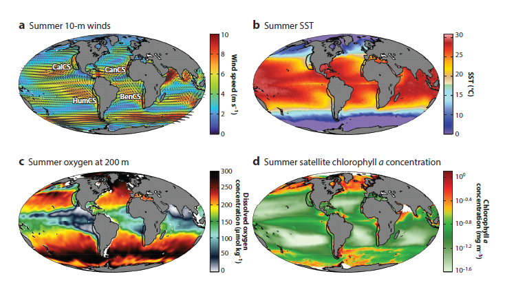
Here on the Oregon Coast, we are perched on the edge of a bountiful upwelling ecosystem. Upwelling is the process by which winds drive a net movement of surface water offshore, which is replaced by cold, nutrient-rich water. When this water full of nutrients meets the sunlight of the photic zone, large phytoplankton blooms occur that sustain high densities of forage species like zooplankton and fish, and yielding important feeding opportunities for predators such as marine mammals. Upwelling ecosystems, like the California Current system in our back yard that features in Duncan Berry’s poem, support over 20% of global fisheries catches despite covering an area less than 5% of the global oceans4–6. These narrow bands of ocean on the eastern boundaries of the major oceans are characterized by strong winds, cool sea surface temperatures, and high primary productivity that ultimately support thriving and productive ecosystems (Fig. 2)7.
Figure 2. Reproduced from Bograd et al. 2023. Maps showing global means in several key properties during the warm season (June through August in the Northern Hemisphere and January through March in the Southern Hemisphere). The locations of the four eastern boundary current upwelling systems (EBUSs) are shown by black outlines in each panel. (a) 10-m wind speed (colors) and vectors. (b) SST. (c) Dissolved oxygen concentrations at 200-m depth. (d) Concentration of ocean chlorophyll a. Abbreviations: BenCS, Benguela Current System; CalCS, California Current System; CanCS, Canary Current System; HumCS, Humboldt Current System; SST, sea surface temperature.
Because of their importance to human societies, eastern boundary current upwelling systems (EBUSs) have been well-studied over time. Now, scientists around the world who have dedicated their careers to understanding and describing the dynamics of upwelling systems are forced to reckon with the looming question of what will happen to these systems under climate change. The state of available information was recently synthesized in a forthcoming paper by Bograd et al. (2023). These authors find that the future of upwelling systems is uncertain, as climate change is anticipated to drive conflicting physical changes in their oceanography. Namely, alongshore winds could increase, which would yield increased upwelling. However, a poleward shift in these upwelling systems will likely lead to long-term changes in the intensity, location, and seasonality of upwelling-favorable winds, with intensification in poleward regions but weakening in equatorward areas. Another projected change is stronger temperature gradients between inshore and offshore areas, and vertically within the water column. What these various opposing forces will mean for primary productivity and species community structure remains to be seen.
While most of my prior research has centered around the importance of productive upwelling systems for supporting marine mammal feeding grounds8–10, my recent focus has shifted closer to home, to the nearshore waters less than 5 km from the coastline. Despite their ecological and economic importance, nearshore habitats remain understudied, particularly in the context of climate change. Through the recently launched EMERALD project, we are investigating spatial and temporal distribution patterns of harbor porpoises and gray whales between San Francisco Bay and the Columbia River in relation to fluctuations in key environmental drivers over the past 30 years. On a scientific level, I am thrilled to have such a rich dataset that enables asking broad questions relating to how changing environmental conditions have impacted these nearshore sentinel species. On a more personal level, I must admit some apprehension of what we will find. The excitement of detecting statistically significant northward shift in harbor porpoise distribution stands at odds with my own grappling with what that means for our planet. The oceans are changing, and sensitive species must move or adapt to persist. What does the future hold for this “wild edge of a continent of ours” that I love, as Duncan Berry describes?
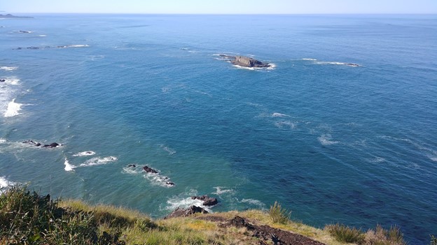
Figure 4. The view from Cape Foulweather, showing the complex mosaic of nearshore habitat features. Photo: D. Barlow.
Evidence exists that the nearshore realm of the Northeast Pacific is actually decoupled from coastal upwelling processes11. Rather, these areas may be a “sweet spot” in the coastal boundary layer where headlands and rocky reefs provide more stable retention areas of productivity, distinct from the strong upwelling currents just slightly further from shore (Fig. 4). As the oceans continue to shift under the impacts of climate change, what will it mean for these critically important nearshore habitats? While they are adjacent to prominent upwelling systems, they are also physically, biologically, and ecologically distinct. Will nearshore habitats act as a refuge alongside a more rapidly changing upwelling environment, or will they be impacted in some different way? Many unanswered questions remain. I am eager to continue seeking out truth in the data, with my drive for scientific inquiry fueled by my underlying connection to this wild edge of a continent that I call home.
Did you enjoy this blog? Want to learn more about marine life, research, and conservation? Subscribe to our blog and get a weekly alert when we make a new post! Just add your name into the subscribe box below!
References:
1. Poloczanska, E. S. et al. Global imprint of climate change on marine life. Nat. Clim. Chang.3, (2013).
2. Lenoir, J. et al. Species better track climate warming in the oceans than on land. Nat. Ecol. Evol.4, 1044–1059 (2020).
3. Hoegh-Guldberg, O. & Bruno, J. F. The impact of climate change on the world’s marine ecosystems. Science (2010). doi:10.1126/science.1189930
4. Mann, K. H. & Lazier, J. R. N. Dynamics of Marine Ecosystems: Biological-physical interactions in the oceans. Blackwell Scientific Publications (1996). doi:10.2307/2960585
5. Ryther, J. Photosynthesis and fish production in the sea. Science (80-. ).166, 72–76 (1969).
6. Cushing, D. H. Plankton production and year-class strength in fish populations: An update of the match/mismatch hypothesis. Adv. Mar. Biol.9, 255–334 (1990).
7. Bograd, S. J. et al. Climate Change Impacts on Eastern Boundary Upwelling Systems. Ann. Rev. Mar. Sci.15, 1–26 (2023).
8. Barlow, D. R., Bernard, K. S., Escobar-Flores, P., Palacios, D. M. & Torres, L. G. Links in the trophic chain: Modeling functional relationships between in situ oceanography, krill, and blue whale distribution under different oceanographic regimes. Mar. Ecol. Prog. Ser.642, 207–225 (2020).
9. Barlow, D. R., Klinck, H., Ponirakis, D., Garvey, C. & Torres, L. G. Temporal and spatial lags between wind, coastal upwelling, and blue whale occurrence. Sci. Rep.11, 1–10 (2021).
10. Derville, S., Barlow, D. R., Hayslip, C. & Torres, L. G. Seasonal, Annual, and Decadal Distribution of Three Rorqual Whale Species Relative to Dynamic Ocean Conditions Off Oregon, USA. Front. Mar. Sci.9, 1–19 (2022).
11. Shanks, A. L. & Shearman, R. K. Paradigm lost? Cross-shelf distributions of intertidal invertebrate larvae are unaffected by upwelling or downwelling. Mar. Ecol. Prog. Ser.385, 189–204 (2009).
Dr. KC Bierlich, Postdoctoral Scholar, OSU Department of Fisheries, Wildlife, & Conservation Sciences, Geospatial Ecology of Marine Megafauna (GEMM) Lab
In a previous blog, I discussed the importance of incorporating measurement uncertainty in drone-based photogrammetry, as drones with different sensors, focal length lenses, and altimeters will have varying levels of measurement accuracy. In my last blog, I discussed how to incorporate photogrammetric uncertainty when combining multiple measurements to estimate body condition of baleen whales. In this blog, I will highlight our recent publication in Frontiers in Marine Science (https://doi.org/10.3389/fmars.2022.867258) led by GEMM Lab’s Dr. Leigh Torres, Clara Bird, and myself that used these methods in a collaborative study using imagery from four different drones to compare gray whale body condition on their breeding and feeding grounds (Torres et al., 2022).
Most Eastern North Pacific (ENP) gray whales migrate to their summer foraging grounds in Alaska and the Arctic, where they target benthic amphipods as prey. A subgroup of gray whales (~230 individuals) called the Pacific Coast Feeding Group (PCFG), instead truncates their migration and forages along the coastal habitats between Northern California and British Columbia, Canada (Fig. 1). Evidence from a recent study lead by GEMM Lab’s Lisa Hildebrand (see this blog) found that the caloric content of prey in the PCFG range is of equal or higher value than the main amphipod prey in the Arctic/sub-Arctic regions (Hildebrand et al., 2021). This implies that greater prey density and/or lower energetic costs of foraging in the Arctic/sub-Arctic may explain the greater number of whales foraging in that region compared to the PCFG range. Both groups of gray whales spend the winter months on their breeding and calving grounds in Baja California, Mexico.
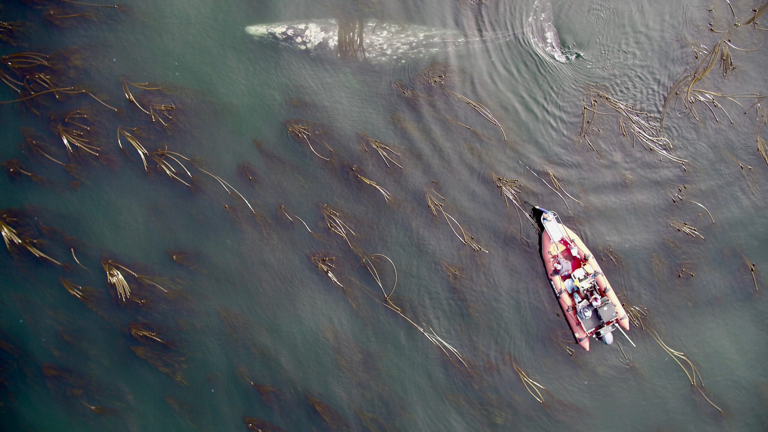
Figure 1. The GEMM Lab field team following a Pacific Coast Feeding Group (PCFG) gray whale swimming in a kelp bed along the Oregon Coast during the summer foraging season.
In January 2019 an Unusual Mortality Event (UME) was declared for gray whales due to the elevated numbers of stranded gray whales between Mexico and the Arctic regions of Alaska. Most of the stranded whales were emaciated, indicating that reduced nutrition and starvation may have been the causal factor of death. It is estimated that the population dropped from ~27,000 individuals in 2016 to ~21,000 in 2020 (Stewart & Weller, 2021).
During this UME period, between 2017-2019, the GEMM Lab was using drones to monitor the body condition of PCFG gray whales on their Oregon coastal feeding grounds (Fig. 1), while Christiansen and colleagues (2020) was using drones to monitor gray whales on their breeding grounds in San Ignacio Lagoon (SIL) in Baja California, Mexico. We teamed up with Christiansen and colleagues to compare the body condition of gray whales in these two different areas leading up to the UME. Comparing the body condition between these two populations could help inform which population was most effected by the UME.
The combined datasets consisted of four different drones used, thus different levels of photogrammetric uncertainty to consider. The GEMM Lab collected data using a DJI Phantom 3 Pro, DJI Phantom 4, and DJI Phantom 4 Pro, while Christiansen et al., (2020) used a DJI Inspire 1 Pro. By using the methodological approach described in my previous blog (here, also see Bierlich et al., 2021a for more details), we quantified photogrammetric uncertainty specific to each drone, allowing cross-comparison between these datasets. We also used Body Area Index (BAI), which is a standardized relative measure of body condition developed by the GEMM Lab (Burnett et al., 2018) that has low uncertainty with high precision, making it easier to detect smaller changes between individuals (see blog here, Bierlich et al., 2021b).
While both PCFG and ENP gray whales visit San Ignacio Lagoon in the winter, we assume that the photogrammetry data collected in the lagoon is mostly of ENP whales based on their considerably higher population abundance. We also assume that gray whales incur low energetic cost during migration, as gray whale oxygen consumption rates and derived metabolic rates are much lower during migration than on foraging grounds (Sumich, 1983).
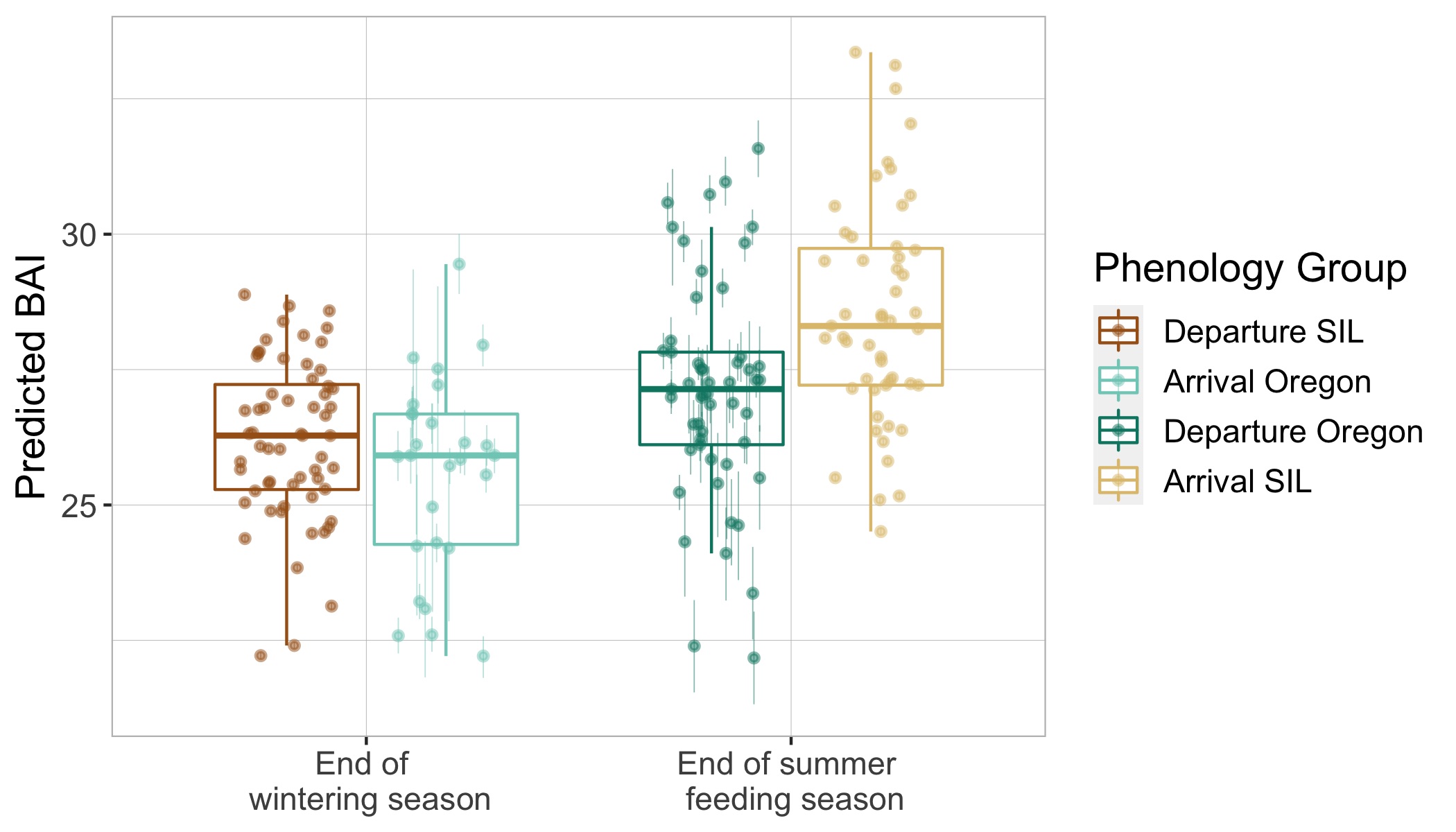
Interestingly, we found that gray whale body condition on their wintering grounds in San Ignacio Lagoon deteriorated across the study years leading up to the UME (2017-2019), while the body condition of PCFG whales on their foraging grounds in Oregon concurrently increased. These contrasting trajectories in body condition between ENP and PCFG whales implies that dynamic oceanographic processes may be contributing to temporal variability of prey available in the Arctic/sub-Arctic and PCFG range. In other words, environmental conditions that control prey availability for gray whales are different in the two areas. For the ENP population, this declining nutritive gain may be associated with environmental changes in the Arctic/sub-Arctic region that impacted the predictability and availability of prey. For the PCFG population, the increase in body condition across years may reflect recovery of the NE Pacific Ocean from the marine heatwave event in 2014-2016 (referred to as “The Blob”) that resulted with a period of low prey availability. These findings also indicate that the ENP population was primarily impacted in the die-off from the UME.
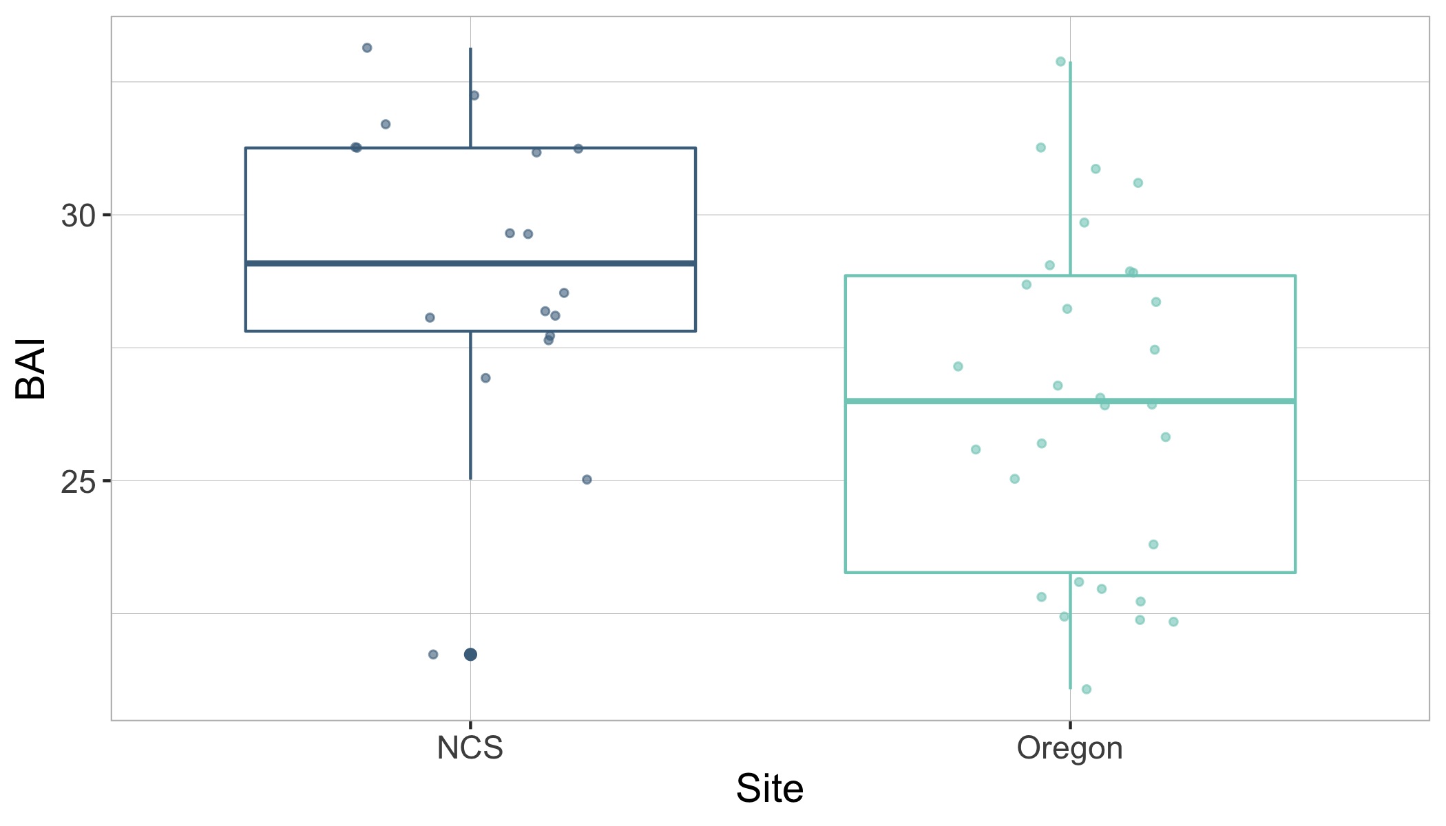
Surprisingly, the body condition of PCFG gray whales in Oregon was regularly and significantly lower than whales in San Ignacio Lagoon (Fig. 2). To further investigate this potential intrinsic difference in body condition between PCFG and ENP whales, we compared opportunistic photographs of gray whales feeding in the Northeastern Chukchi Sea (NCS) in the Arctic collected from airplane surveys. We found that the body condition of PCFG gray whales was significantly lower than whales in the NCS, further supporting our finding that PCFG whales overall have lower body condition than ENP whales that feed in the Arctic (Fig. 3).
Figure 2. Boxplots showing the distribution of Body Area Index (BAI) values for gray whales imaged by drones in San Ignacio Lagoon (SIL), Mexico and Oregon, USA. The data is grouped by phenology group: End of summer feeding season (departure Oregon vs. arrival SIL) and End of wintering season (arrival Oregon vs. departure SIL). The group median (horizontal line), interquartile range (IQR, box), maximum and minimum 1.5*IQR (vertical lines), and outliers (dots) are depicted in the boxplots. The overlaid points represent the mean of the posterior predictive distribution for BAI of an individual and the bars represents the uncertainty (upper and lower bounds of the 95% HPD interval). Note how PCFG whales at then end of the feeding season (dark green) typically have lower body condition (as BAI) compared to ENP whales at the end of the feeding season when they arrive to SIL after migration (light brown).Figure 3. Boxplots showing the distribution of Body Area Index (BAI) values of gray whales from opportunistic images collected from a plane in Northeaster Chukchi Sea (NCS) and from drones collected by the GEMM Lab in Oregon. The boxplots display the group median (horizontal line), interquartile range (IQR box), maximum and minimum 1.5*IQR (vertical lines), and outlies (dots). The overlaid points are the BAI values from each image. Note the significantly lower BAI of PCFG whales on Oregon feeding grounds compared to whales feeding in the Arctic region of the NCS.
This difference in body condition between PCFG and ENP gray whales raises some really interesting and prudent questions. Does the lower body condition of PCFG whales make them less resilient to changes in prey availability compared to ENP whales, and thus more vulnerable to climate change? If so, could this influence the reproductive capacity of PCFG whales? Or, are whales that recruit into the PCFG adapted to a smaller morphology, perhaps due to their specialized foraging tactics, which may be genetically inherited and enables them to survive with reduced energy stores?
These questions are on our minds here at the GEMM Lab as we prepare for our seventh consecutive field season using drones to collect data on PCFG gray whale body condition. As discussed in a previous blog by Dr. Alejandro Fernandez Ajo, we are combining our sightings history of individual whales, fecal hormone analyses, and photogrammetry-based body condition to better understand gray whales’ reproductive biology and help determine what the consequences are for these PCFG whales with lower body condition.
Did you enjoy this blog? Want to learn more about marine life, research, and conservation? Subscribe to our blog and get a weekly message when we post a new blog. Just add your name and email into the subscribe box below.
References
Bierlich, K. C., Hewitt, J., Bird, C. N., Schick, R. S., Friedlaender, A., Torres, L. G., … & Johnston, D. W. (2021). Comparing Uncertainty Associated With 1-, 2-, and 3D Aerial Photogrammetry-Based Body Condition Measurements of Baleen Whales. Frontiers in Marine Science, 1729.
Bierlich, K. C., Schick, R. S., Hewitt, J., Dale, J., Goldbogen, J. A., Friedlaender, A.S., et al. (2021b). Bayesian Approach for Predicting Photogrammetric Uncertainty in Morphometric Measurements Derived From Drones. Mar. Ecol. Prog. Ser. 673, 193–210. doi: 10.3354/meps13814
Burnett, J. D., Lemos, L., Barlow, D., Wing, M. G., Chandler, T., & Torres, L. G. (2018). Estimating morphometric attributes of baleen whales with photogrammetry from small UASs: A case study with blue and gray whales. Marine Mammal Science, 35(1), 108–139.
Christiansen, F., Rodrı́guez-González, F., Martı́nez-Aguilar, S., Urbán, J., Swartz, S., Warick, H., et al. (2021). Poor Body Condition Associated With an Unusual Mortality Event in Gray Whales. Mar. Ecol. Prog. Ser. 658, 237–252. doi:10.3354/meps13585
Hildebrand, L., Bernard, K. S., and Torres, L. G. (2021). Do Gray Whales Count Calories? Comparing Energetic Values of Gray Whale Prey Across Two Different Feeding Grounds in the Eastern North Pacific. Front. Mar. Sci. 8. doi: 10.3389/fmars.2021.683634
Stewart, J. D., and Weller, D. (2021). Abundance of Eastern North Pacific Gray Whales 2019/2020 (San Diego, CA: NOAA/NMFS)
Sumich, J. L. (1983). Swimming Velocities, Breathing Patterns, and Estimated Costs of Locomotion in Migrating Gray Whales, Eschrichtius Robustus. Can. J. Zoology. 61, 647–652. doi: 10.1139/z83-086
Torres, L.G., Bird, C., Rodrigues-Gonzáles, F., Christiansen F., Bejder, L., Lemos, L., Urbán Ramírez, J., Swartz, S., Willoughby, A., Hewitt., J., Bierlich, K.C. (2022). Range-wide comparison of gray whale body condition reveals contrasting sub-population health characteristics and vulnerability to environmental change. Frontiers in Marine Science. 9:867258. https://doi.org/10.3389/fmars.2022.867258
2MS Student, OSU Department of Fisheries, Wildlife, and Conservation Sciences, Seabird Oceanography Lab
The marine environment is dynamic, and mobile animals must respond to the patchy and ephemeral availability of resource in order to make a living (Hyrenbach et al. 2000). Climate change is making ocean ecosystems increasingly unstable, yet these novel conditions can be difficult to document given the vast depth and remoteness of most ocean locations. Marine megafauna species such as marine mammals and seabirds integrate ecological processes that are often difficult to observe directly, by shifting patterns in their distribution, behavior, physiology, and life history in response to changes in their environment (Croll et al. 1998, Hazen et al. 2019). These mobile marine animals now face additional challenges as rising temperatures due to global climate change impact marine ecosystems worldwide (Hazen et al. 2013, Sydeman et al. 2015, Silber et al. 2017, Becker et al. 2019). Given their mobility, visibility, and integration of ocean processes across spatial and temporal scales, these marine predator species have earned the reputation as effective ecosystem sentinels. As sentinels, they have the capacity to shed light on ecosystem function, identify risks to human health, and even predict future changes (Hazen et al. 2019). So, let’s explore a few examples of how studying marine megafauna has revealed important new insights, pointing toward the importance of monitoring these sentinels in a rapidly changing ocean.
Cairns (1988) is often credited as first promoting seabirds as ecosystem sentinels and noted several key reasons why they were perfect for this role: (1) Seabirds are abundant, wide-ranging, and conspicuous, (2) although they feed at sea, they must return to land to nest, allowing easier observation and quantification of demographic responses, often at a fraction of the cost of traditional, ship-based oceanographic surveys, and therefore (3) parameters such as seabird reproductive success or activity budgets may respond to changing environmental conditions and provide researchers with metrics by which to assess the current state of that ecosystem.
The unprecedented 2014-2016 North Pacific marine heatwave (“the Blob”) caused extreme ecosystem disruption over an immense swath of the ocean (Cavole et al. 2016). Seabirds offered an effective and morbid indication of the scale of this disruption: Common murres (Uria aalge), an abundant and widespread fish-eating seabird, experienced widespread breeding failure across the North Pacific. Poor reproductive performance suggested that there may have been fewer small forage fish around and that these changes occurred at a large geographic scale. The Blob reached such an extreme as to kill immense numbers of adult birds, which professional and community scientists found washed up on beach-surveys; researchers estimate that an incredible 1,200,000 murres may have died from starvation during this period (Piatt et al. 2020). While the average person along the Northeast Pacific Coast during this time likely didn’t notice any dramatic difference in the ocean, seabirds were shouting at us that something was terribly wrong.
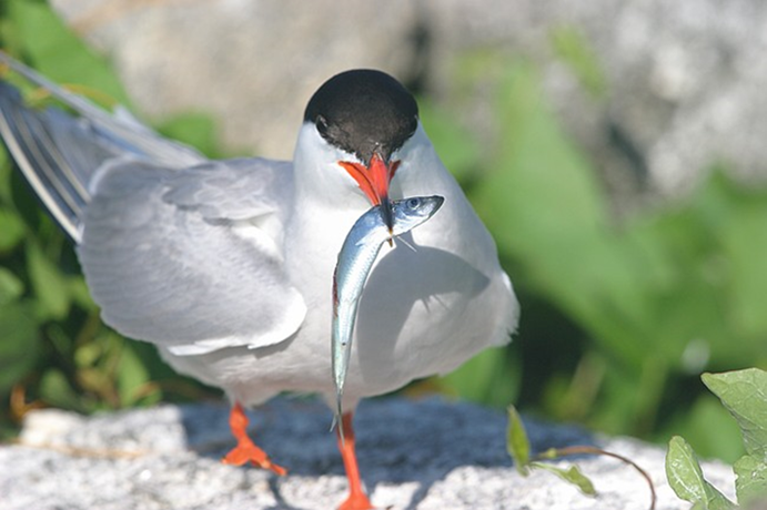
Happily, living seabirds also act as superb ecosystem sentinels. Long-term research in the Gulf of Maine by U.S. and Canadian scientists monitors the prey species provisioned by adult seabirds to their chicks. Will has spent countless hours over five summers helping to conduct this research by watching terns (Sterna spp.) and Atlantic puffins (Fratercula arctica) bring food to their young on small islands off the Maine coast. After doing this work for multiple years, it’s easy to notice that what adults feed their chicks varies from year to year. It was soon realized that these data could offer insight into oceanographic conditions and could even help managers assess the size of regional fish stocks. One of the dominant prey species in this region is Atlantic herring (Clupea harengus), which also happens to be the focus of an economically important fishery. While the fishery targets four or five-year-old adult herring, the seabirds target smaller, younger herring. By looking at the relative amounts and sizes of young herring collected by these seabirds in the Gulf of Maine, these data can help predict herring recruitment and the relative number of adult herring that may be available to fishers several years in the future (Scopel et al. 2018). With some continued modelling, the work that we do on a seabird colony in Maine with just a pair of binoculars can support or maybe even replace at least some of the expensive ship-based trawl surveys that are now a popular means of assessing fish stocks.
A common tern (Sterna hirundo) with a young Atlantic herring from the Gulf of Maine, ready to feed its chick (Photo courtesy of the National Audubon Society’s Seabird Institute)
For more far-ranging and inaccessible marine predators such as whales, measuring things such as dietary shifts can be more challenging than it is for seabirds. Nevertheless, whales are valuable ecosystem sentinels as well. Changes in the distribution and migration phenology of specialist foragers such as blue whales (Balaenoptera musculus) and North Atlantic right whales (Eubalaena glacialis) can indicate relative changes in the distribution and abundance of their zooplankton prey and underlying ocean conditions (Hazen et al. 2019). In the case of the critically endangered North Atlantic right whale, their recent declines in reproductive success reflect a broader regime shift in climate and ocean conditions. Reduced copepod prey has resulted in fewer foraging opportunities and changing foraging grounds, which may be insufficient for whales to obtain necessary energetic stores to support calving (Gavrilchuk et al. 2021, Meyer-Gutbrod et al. 2021). These whales assimilate and showcase the broad-scale impacts of climate change on the ecosystem they inhabit.
Blue whales that feed in the rich upwelling system off the coast of California rely on the availability of their krill prey to support the population (Croll et al. 2005). A recent study used acoustic monitoring of blue whale song to examine the timing of annual population-level transition from foraging to breeding migration compared to oceanographic variation, and found that flexibility in timing may be a key adaptation to persistence of this endangered population facing pressures of rapid environmental change (Oestreich et al. 2022). Specifically, blue whales delayed the transition from foraging to breeding migration in years of the highest and most persistent biological productivity from upwelling, and therefore listening to the vocalizations of these whales may be valuable indicator of the state of productivity in the ecosystem.
Figure reproduced from Oestreich et al. 2022, showing relationships between blue whale life-history transition and oceanographic phenology of foraging habitat. Timing of the behavioral transition from foraging to migration (day of year on the y-axis) is compared to (a) the date of upwelling onset; (b) the date of peak upwelling; and (c) total upwelling accumulated from the spring transition to the end of the upwelling season.
In a similar vein, research by the GEMM Lab on blue whale ecology in New Zealand has linked their vocalizations known as D calls to upwelling conditions, demonstrating that these calls likely reflect blue whale foraging opportunities (Barlow et al. 2021). In ongoing analyses, we are finding that these foraging-related calls were drastically reduced during marine heatwave conditions, which we know altered blue whale distribution in the region (Barlow et al. 2020). Now, for the final component of Dawn’s PhD, she is linking year-round environmental conditions to the occurrence patterns of different blue whale vocalization types, hoping to shed light on ecosystem processes by listening to the signals of these ecosystem sentinels.
A blue whale comes up for air in the South Taranaki Bight of New Zealand. photo by L. Torres.
It is important to understand the widespread implications of the rapidly warming climate and changing ocean conditions on valuable and vulnerable marine ecosystems. The cases explored here in this blog exemplify the importance of monitoring these marine megafauna sentinel species, both now and into the future, as they reflect the health of the ecosystems they inhabit.
Did you enjoy this blog? Want to learn more about marine life, research and conservation? Subscribe to our blog and get a weekly email when we make a new post! Just add your name into the subscribe box on the left panel.
References:
Barlow DR, Bernard KS, Escobar-Flores P, Palacios DM, Torres LG (2020) Links in the trophic chain: Modeling functional relationships between in situ oceanography, krill, and blue whale distribution under different oceanographic regimes. Mar Ecol Prog Ser 642:207–225.
Barlow DR, Klinck H, Ponirakis D, Garvey C, Torres LG (2021) Temporal and spatial lags between wind, coastal upwelling, and blue whale occurrence. Sci Rep 11:1–10.
Becker EA, Forney KA, Redfern J V., Barlow J, Jacox MG, Roberts JJ, Palacios DM (2019) Predicting cetacean abundance and distribution in a changing climate. Divers Distrib 25:626–643.
Cairns DK (1988) Seabirds as indicators of marine food supplies. Biol Oceanogr 5:261–271.
Cavole LM, Demko AM, Diner RE, Giddings A, Koester I, Pagniello CMLS, Paulsen ML, Ramirez-Valdez A, Schwenck SM, Yen NK, Zill ME, Franks PJS (2016) Biological impacts of the 2013–2015 warm-water anomaly in the northeast Pacific: Winners, losers, and the future. Oceanography 29:273–285.
Croll DA, Marinovic B, Benson S, Chavez FP, Black N, Ternullo R, Tershy BR (2005) From wind to whales: Trophic links in a coastal upwelling system. Mar Ecol Prog Ser 289:117–130.
Croll DA, Tershy BR, Hewitt RP, Demer DA, Fiedler PC, Smith SE, Armstrong W, Popp JM, Kiekhefer T, Lopez VR, Urban J, Gendron D (1998) An integrated approch to the foraging ecology of marine birds and mammals. Deep Res Part II Top Stud Oceanogr.
Gavrilchuk K, Lesage V, Fortune SME, Trites AW, Plourde S (2021) Foraging habitat of North Atlantic right whales has declined in the Gulf of St. Lawrence, Canada, and may be insufficient for successful reproduction. Endanger Species Res 44:113–136.
Hazen EL, Abrahms B, Brodie S, Carroll G, Jacox MG, Savoca MS, Scales KL, Sydeman WJ, Bograd SJ (2019) Marine top predators as climate and ecosystem sentinels. Front Ecol Environ 17:565–574.
Hazen EL, Jorgensen S, Rykaczewski RR, Bograd SJ, Foley DG, Jonsen ID, Shaffer SA, Dunne JP, Costa DP, Crowder LB, Block BA (2013) Predicted habitat shifts of Pacific top predators in a changing climate. Nat Clim Chang 3:234–238.
Hyrenbach KD, Forney KA, Dayton PK (2000) Marine protected areas and ocean basin management. Aquat Conserv Mar Freshw Ecosyst 10:437–458.
Meyer-Gutbrod EL, Greene CH, Davies KTA, Johns DG (2021) Ocean regime shift is driving collapse of the north atlantic right whale population. Oceanography 34:22–31.
Oestreich WK, Abrahms B, Mckenna MF, Goldbogen JA, Crowder LB, Ryan JP (2022) Acoustic signature reveals blue whales tune life history transitions to oceanographic conditions. Funct Ecol.
Piatt JF, Parrish JK, Renner HM, Schoen SK, Jones TT, Arimitsu ML, Kuletz KJ, Bodenstein B, Garcia-Reyes M, Duerr RS, Corcoran RM, Kaler RSA, McChesney J, Golightly RT, Coletti HA, Suryan RM, Burgess HK, Lindsey J, Lindquist K, Warzybok PM, Jahncke J, Roletto J, Sydeman WJ (2020) Extreme mortality and reproductive failure of common murres resulting from the northeast Pacific marine heatwave of 2014-2016. PLoS One 15:e0226087.
Scopel LC, Diamond AW, Kress SW, Hards AR, Shannon P (2018) Seabird diets as bioindicators of atlantic herring recruitment and stock size: A new tool for ecosystem-based fisheries management. Can J Fish Aquat Sci.
Silber GK, Lettrich MD, Thomas PO, Baker JD, Baumgartner M, Becker EA, Boveng P, Dick DM, Fiechter J, Forcada J, Forney KA, Griffis RB, Hare JA, Hobday AJ, Howell D, Laidre KL, Mantua N, Quakenbush L, Santora JA, Stafford KM, Spencer P, Stock C, Sydeman W, Van Houtan K, Waples RS (2017) Projecting marine mammal distribution in a changing climate. Front Mar Sci 4:413.
Sydeman WJ, Poloczanska E, Reed TE, Thompson SA (2015) Climate change and marine vertebrates. Science 350:772–777.
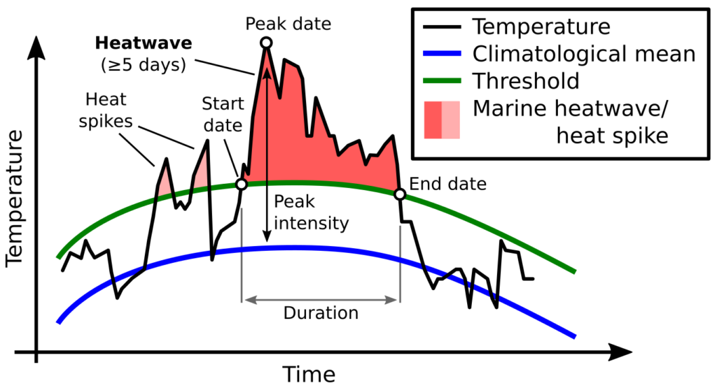
In recent years, anomalously warm ocean temperatures known as “marine heatwaves” have sparked considerable attention and concern around the world. Marine heatwaves (MHW) occur when seawater temperatures rise above a seasonal threshold (greater than the 90th percentile) for five consecutive days or longer (Hobday et al. 2016; Fig. 1). With global ocean temperatures continuing to rise, we are likely to see more frequent and more intense MHW conditions in the future. Indeed, the global prevalence of MHWs is increasing, with a 34% rise in frequency, a 17% increase in duration, and a 54% increase in annual MHW days globally since 1925 (Oliver et al. 2018). With sustained anomalously warm water temperatures come a range of ecological, sociological, and economic consequences. These impacts include changes in water column structure, primary production, species composition, marine life distribution and health, and fisheries management including closures and quota changes (Oliver et al. 2018).
Figure 1. Illustration of how marine heatwaves are defined. Source: marineheatwaves.org
The notorious “warm blob” was an MHW event that plagued the northeast Pacific Ocean from 2014-2016. Some of the most notable consequences of this MHW were extremely high levels of domoic acid, extreme changes in the biodiversity of pelagic species, and an unprecedented delay in the opening of the Dungeness crab fishery, which is an important and lucrative fishery for the West Coast of the United States (Santora et al. 2020). The “warm blob” directly impacted the California Current ecosystem, which is typically a highly productive coastal area driven by seasonal upwelling. Yet, as a consequence of the 2014-2016 MHW, upwelling habitat was compressed and constricted to the coastal boundary, resulting in a contraction in available habitat for humpback whales and a shift in their prey (Santora et al. 2020; Fig. 2).
Figure 2. A figure from Santora et al. 2020 illustrating the compression in available upwelling habitat, defined by areas with SST<12°C (delineated by the black line), during the 2014-2016 marine heatwave in the California Current ecosystem.
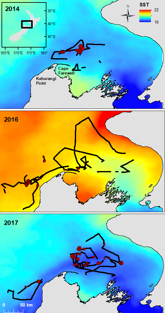
Shifting to an example from another part of the world, the austral summer of 2015-2016 coincided with a strong regional MHW in the Tasman Sea between Australia and New Zealand, which lasted for 251 days and had a maximum intensity of 2.9°C above the climatological average (Oliver et al. 2017). Subsequently, the conditions were linked to a significant shift in zooplankton species composition and abundance in Australia (Evans et al. 2020). Ocean warming, including MHWs, also appears to decrease primary production in the Tasman Sea and large portions of New Zealand’s marine ecosystem (Chiswell & Sutton 2020). In New Zealand’s South Taranaki Bight region, where we study the ecology of blue whales, we observed a shift in blue whale distribution in the MWH conditions of February 2016 relative to more typical ocean conditions in 2014 and 2017 (Fig. 3). The first chapter of my dissertation includes a detailed analysis of the impacts of the 2016 MHW on New Zealand oceanography, krill, and blue whales, documenting how the warm, stratified water column of 2016 led to consequences across multiple trophic levels, from phytoplankton, to zooplankton, to whales.
Figure 3. Maps showing monthly sea surface temperature (SST) in the South Taranaki Bight region of New Zealand during our three years of survey effort to document blue whale distribution (February 2014, 2016, and 2017). Vessel tracklines are shown in black, with blue whale sighting locations shown in dark red. Red circles are scaled by the number of blue whales observed at each sighting. The color ramp of SST values is consistent across the three maps, making the dramatically warmer ocean conditions of 2016 evident.
The response of marine mammals is tightly linked to shifts in their environment and prey (Silber et al. 2017). With MHWs and changing ocean conditions, there will likely be “winners” and “losers” among marine predators including large whales. Blue whales are highly selective krill specialists (Nickels et al. 2019), whereas other species of whales, such as humpback whales, have evolved flexible feeding tactics that allow them to switch target prey species when needed (Cade et al. 2020). In California, humpback whales have been shown to switch their primary prey from krill to fish during warm years (Fossette et al. 2017, Santora et al. 2020). By contrast, blue whales shift their distribution in response to changing krill availability during warm years (Fossette et al. 2017), however this strategy comes with increased risk and energetic cost associated with searching for prey in new areas. Furthermore, in instances when a prey resource such as krill becomes increasingly scarce for a multi-year period (Santora et al. 2020), krill specialist predators such as blue whales are at a considerable disadvantage. It is also important to acknowledge that although the humpbacks in California may at first seem to have a winning strategy for adaptation by switching their food source, this tactic may come with unforeseen consequences. Their distribution overlapped substantially with Dungeness crab fishing gear during MHW conditions in the warm blob years, resulting in record numbers of entanglements that may have population-level repercussions (Santora et al. 2020).
While this is certainly not the most light-hearted blog
topic, I believe it is an important one. As warming ocean temperatures
contribute to the increase in frequency, intensity, and duration of extreme
conditions such as MHW events, it is paramount that we understand their impacts
and take informed management actions to mitigate consequences, such as lethal
entanglements as a result of compressed whale habitat. But perhaps more
importantly, even as we do our best to manage consequences, it is critical that
we as individuals realize the role we have to play in reducing the root cause
of warming oceans, by being conscious consumers and being mindful of the impact
our actions have on the climate.
References
Cade DE, Carey N, Domenici P, Potvin J, Goldbogen JA (2020) Predator-informed looming stimulus experiments reveal how large filter feeding whales capture highly maneuverable forage fish. Proc Natl Acad Sci USA.
Chiswell SM, Sutton PJH
(2020) Relationships between long-term ocean warming, marine heat waves and
primary production in the New Zealand region. New Zeal J Mar Freshw Res.
Evans R, Lea MA, Hindell
MA, Swadling KM (2020) Significant shifts in coastal zooplankton populations
through the 2015/16 Tasman Sea marine heatwave. Estuar Coast Shelf Sci.
Fossette S, Abrahms B,
Hazen EL, Bograd SJ, Zilliacus KM, Calambokidis J, Burrows JA, Goldbogen JA,
Harvey JT, Marinovic B, Tershy B, Croll DA (2017) Resource partitioning
facilitates coexistence in sympatric cetaceans in the California Current. Ecol
Evol.
Hobday AJ, Alexander L
V., Perkins SE, Smale DA, Straub SC, Oliver ECJ, Benthuysen JA, Burrows MT,
Donat MG, Feng M, Holbrook NJ, Moore PJ, Scannell HA, Sen Gupta A, Wernberg T
(2016) A hierarchical approach to defining marine heatwaves. Prog Oceanogr.
Nickels CF, Sala LM,
Ohman MD (2019) The euphausiid prey field for blue whales around a steep
bathymetric feature in the southern California current system. Limnol Oceanogr.
Oliver ECJ, Benthuysen
JA, Bindoff NL, Hobday AJ, Holbrook NJ, Mundy CN, Perkins-Kirkpatrick SE (2017)
The unprecedented 2015/16 Tasman Sea marine heatwave. Nat Commun.
Oliver ECJ, Donat MG,
Burrows MT, Moore PJ, Smale DA, Alexander L V., Benthuysen JA, Feng M, Sen
Gupta A, Hobday AJ, Holbrook NJ, Perkins-Kirkpatrick SE, Scannell HA, Straub
SC, Wernberg T (2018) Longer and more frequent marine heatwaves over the past
century. Nat Commun.
Santora JA, Mantua NJ,
Schroeder ID, Field JC, Hazen EL, Bograd SJ, Sydeman WJ, Wells BK, Calambokidis
J, Saez L, Lawson D, Forney KA (2020) Habitat compression and ecosystem shifts
as potential links between marine heatwave and record whale entanglements. Nat
Commun.
Silber GK, Lettrich MD,
Thomas PO, Baker JD, Baumgartner M, Becker EA, Boveng P, Dick DM, Fiechter J,
Forcada J, Forney KA, Griffis RB, Hare JA, Hobday AJ, Howell D, Laidre KL,
Mantua N, Quakenbush L, Santora JA, Stafford KM, Spencer P, Stock C, Sydeman W,
Van Houtan K, Waples RS (2017) Projecting marine mammal distribution in a
changing climate. Front Mar Sci.
1Masters Student in Marine Resource Management, 2Doctoral Student in Integrative Biology
Five years ago, the North Pacific Ocean
experienced a sudden increase in sea surface temperature (SST), known as the
warm blob, which altered marine ecosystem function and structure (Leising et
al. 2015). Much research illustrated how the warm blob impacted pelagic
ecosystems, with relatively less focused on the nearshore environment. Yet, a
new study demonstrated how rising ocean temperatures have partially led to
bull kelp loss in northern California. Unfortunately, we are once again observing
similar warming trends, representing the second largest marine heatwave
over recent decades, and signaling the potential rise of a second warm blob. Taken
together, all these findings could forecast future warming-related ecosystem
shifts in Oregon, highlighting the need for scientists and managers to consider
strategies to prevent future kelp loss, such as reintroducing sea otters.
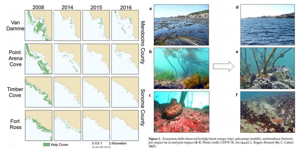
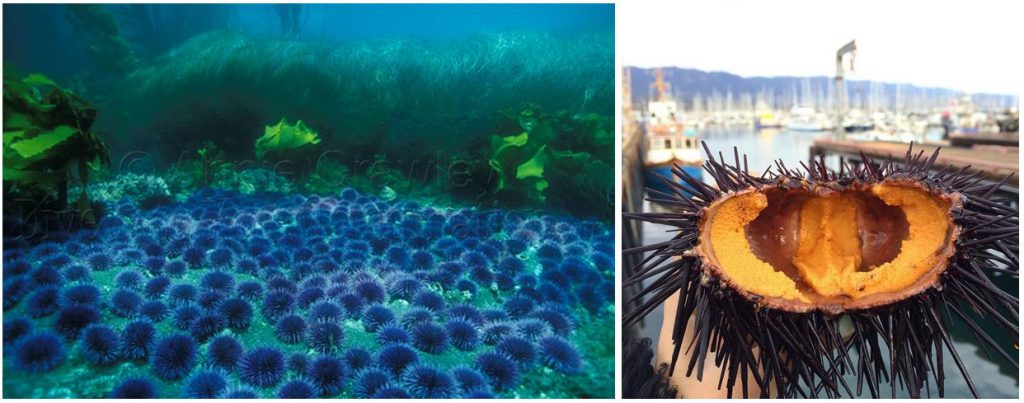
In northern California, researchers observed a dramatic
ecosystem shift from productive bull kelp forests to purple sea urchin barrens.
The study, led by Dr. Laura Rogers-Bennett from the University of California,
Davis and California Department of Fish and Wildlife, determined that this
shift was caused by multiple climatic and biological stressors. Beginning in
2013, sea star populations were decimated by sea star wasting
disease (SSWD). Sea stars are a main predator of urchins, causing their
absence to release purple urchins from predation pressure. Then, starting in
2014, ocean temperatures spiked with the warm blob. These two events created
nutrient-poor conditions, which limited kelp growth and productivity, and allowed
purple urchin populations to grow unchecked by predators and increase grazing
on bull kelp. The combined effect led to approximately 90% reductions in bull
kelp, with a reciprocal 60-fold increase in purple urchins (Figure 1).
Figure 1. Kelp loss and ecosystem shifts in northern California (Rogers-Bennett & Catton 2019).
These changes have wrought economic challenges as
well as ecological collapse in Northern California. Bull kelp is important habitat
and food source for several species of economic importance including red
abalone and red sea urchins (Tegner & Levin 1982). Without bull kelp, red
abalone and red sea urchin populations have starved, resulting in the subsequent
loss of the recreational red abalone ($44 million) and commercial red sea
urchin fisheries in Northern California. With such large kelp reductions,
purple urchins are also now in a starved state, evidenced by noticeably smaller
gonads (Rogers-Bennett & Catton 2019).
Biogeographically, southern Oregon is very similar
to northern California, as both are composed of complex rocky substrates and
shorelines, bull kelp canopies, and benthic macroinvertebrates (i.e. sea
urchins, abalone, etc.). Because Oregon was also impacted by the 2014-2015 warm
blob and SSWD, we might expect to see a similar coastwide kelp forest loss
along our southern coastline. The story is more complicated than that, however.
For instance, ODFW
has found purple urchin barrens where almost no kelp remains in some
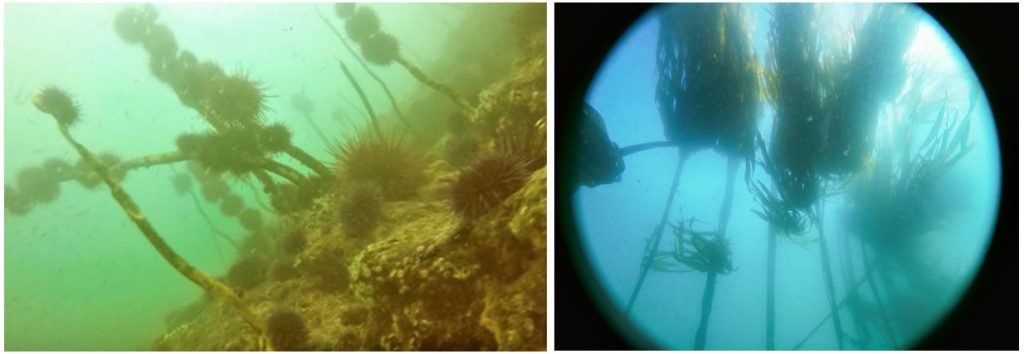
localized places. The GEMM Lab has video footage of purple urchins climbing up
kelp stalks to graze within one of these barrens near Port Orford, OR (Figure 2,
left). In her study, Dr. Rogers-Bennett explains that this aggressive sea
urchin feeding strategy is potentially a sign of food limitation, where
high-density urchin populations create intense resource competition. Conversely,
at sites like Lighthouse Reef (~45 km from Port Orford) outside Charleston, OR,
OSU and University of Oregon divers are currently seeing flourishing bull kelp
forests. Urchins at this reef have fat, rich gonads, which is an indicator of
high-quality nutrition (Figure 2, right).
Satellites can detect kelp on the surface of the
water, giving scientists a way to track kelp extent over time. Preliminary
results from Sara Hamilton’s Ph.D. thesis research finds that while some kelp
forests have shrunk in past years, others are currently bigger than ever in the
last 35 years. It is not clear what is driving this spatial variability in
urchin and kelp populations, nor why southern Oregon has not yet faced the same
kind of coastwide kelp forest collapse as northern California. Regardless, it
is likely that kelp loss in both northern California and southern Oregon may be
triggered and/or exacerbated by rising temperatures.
Figure 2. Left: Purple urchin aggressive grazing near Port Orford, OR (GEMM Lab 2019). Right: Flourishing bull kelp near Charleston, OR (Sara Hamilton 2019).
The reintroduction of sea otters has been proposed
as a solution to combat rising urchin populations and bull kelp loss in Oregon.
From an ecological perspective, there is some validity to this idea. Sea otters
are a voracious urchin predator that routinely reduce urchin populations and
alleviate herbivory on kelp (Estes & Palmisano 1974). Such restoration and
protection of bull kelp could help prevent red abalone and red sea urchin starvation.
Additionally, restoring apex predators and increasing species richness is often
linked to increased ecosystem resilience, which is particularly important in
the face of global anthropogenic change (Estes et al. 2011)
While sea otters could alleviate grazing pressure
on Oregon’s bull kelp, this idea only looks at the issue from a top-down, not bottom-up,
perspective. Sea otters require a lot of food (Costa 1978, Reidman & Estes
1990), and what they eat will always be a function of prey availability and
quality (Ostfeld 1982). Just because urchins are available, doesn’t mean otters
will eat them. In fact, sea otters prefer large and heavy (i.e. high gonad
content) urchins (Ostfeld 1982). In the field, researchers have observed sea
otters avoiding urchins at the center of urchin barrens (personal
communication), presumably because those urchins have less access to kelp beds than
on the barren periphery, and therefore, are constantly in a starved state (Konar
& Estes 2003) (Figure 3). These findings suggest prey quality is more
important to sea otter survival than just prey abundance.
Purple urchin quality has not been widely assessed
in Oregon, but early results show that gonad size varies widely depending on
urchin density and habitat type. In places where urchin barrens have formed,
like Port Orford, purple urchins are likely starving and thus may be a poor
source of nutrition for sea otters. Before we decide whether sea otters are a
viable tool to combat kelp loss, prey surveys may need to be conducted to
assess if a sea otter population could be sustained based on their caloric
requirements. Furthermore, predictions of how these prey populations may change
due to rising temperatures could help determine the potential for sea otters to
become reestablished in Oregon under rapid environmental change.
Recent events in California could signal
climate-driven processes that are already impacting some parts of Oregon and could
become more widespread. Dr. Rogers-Bennett’s study is valuable as she has quantified
and described ecosystem changes that might occur along Oregon’s southern
coastline. The resurgence of a potential second warm blob and the frequency
between these warming events begs the question if such temperature spikes are
still anomalous or becoming the norm. If the latter, we could see more
pronounced kelp loss and major shifts in nearshore ecosystem baselines, where function
and structure is permanently altered. Whether reintroducing sea otters can
prevent these changes will ultimately depend on prey and habitat availability
and quality, and should be carefully considered.
References:
Costa, D. P. 1978. The ecological energetics,
water, and electrolyte balance of the California sea otter (Enhydra lutris).
Ph.D. dissertation, University of California, Santa Cruz.
Estes, J. A. and J.F. Palmisano. 1974. Sea
otters: their role in structuring nearshore communities. Science. 185(4156):
1058-1060.
Estes et al. 2011. Trophic downgrading of planet Earth. Science. 333(6040): 301-306.
Harvell et al. 2019. Disease epidemic and a
marine heat wave are associated with the continental-scale collapse of a
pivotal predator (Pycnopodia helianthoides). Science Advances.
5(1).
Konar, B., and J. A. Estes. 2003. The stability of
boundary regions between kelp beds and deforested areas. Ecology. 84(1):
174-185.
Leising et al. 2015. State of California Current
2014-2015: impacts of the warm-water “blob”. CalCOFI Reports. (56):
31-68.
Ostfeld, R. S. 1982. Foraging strategies and prey
switching in the California sea otter. Oecologia. 53(2):
170-178.
Reidman, M. L. and J. A. Estes. 1990. The sea
otter (Enhydra lutris): behavior, ecology, and natural history. United
States Department of the Interior, Fish and Wildlife Service, Biological
Report. 90: 1-126.
Rogers-Bennett, L., and C. A. Catton. 2019. Marine
heat wave and multiple stressors tip bull kelp forest to sea urchin barrens. Scientific
Reports. 9:15050.
Tegner, M. J., and L. A. Levin. 1982. Do sea
urchins and abalones compete in California? International Echinoderms
Conference, Tampa Bay. J. M Lawrence, ed.