Blue whales – Geospatial Ecology of Marine Megafauna Laboratory

Burning Krillories – Determining Krill Caloric Content in New Zealand’s South Taranaki Bight

By Nina Mahalingam, University of California Davis, OSU CEOAS REU program

Hello! I’m Nina Mahalingam, a rising junior at the University of California, Davis studying biochemistry and molecular biology. Growing up in New Hampshire and Massachusetts, the Boston Aquarium was practically in my backyard – and with just one feel of a touch tank, a lifelong affinity for marine sciences began. CEOAS has provided me with a grand opportunity to pursue this passion, and I can’t wait to dip my toes into the salt water!

Figure 1. Nina posing with a Parr Semimicro Calorimeter.

Here at OSU, I’m researching how our tiny friends, the krill, can provide a krill-uminating perspective on trophic ecology and the vitality of marine ecosystems by investigating the caloric content of an understudied species of krill off the coast of New Zealand. Nyctiphanes australis serves as a key prey species to numerous higher trophic levels. Limited knowledge exists regarding the distribution of N. australis in the South Taranaki Bight (STB), with only a handful of studies focused exclusively on the species. The majority of recent information available on the species in the STB came out of research on blue whales and their foraging behaviors (e.g., Barlow et al., 2020). However, given that the spatial distribution of N. australis directly influences the distribution of predator species that depend on them for sustenance (Barlow et. al. 2020), studying the krill may yield a more comprehensive understanding of blue whale behavior as well as ecosystem resilience.

Figure 2. Nyctiphances australis. Photo by A. Slotwinski, CSIRO.

Seawater temperatures around New Zealand have been increasing since 1981 (Sutton & Bowen, 2019), and there is a growing concern about the implications to marine life. In particular, increasing ocean temperatures have had significant impacts on local aquaculture and fisheries (Sutton et al. 2005; Bowen et al. 2017). Although warming trends along the North Island, north of East Cape, have been more severe (around 0.4℃ increase per decade), warming has also been observed in the central and western areas of the STB, averaging around 0.15-0.20℃ increase per decade (Sutton & Bowen, 2019). During Marine Heat Waves (MHWs) (data collected between 2002 and 2018), warming anomalies were observed to decrease phytoplankton presence (Chiswell & Sutton, 2020). Being krill’s primary food source, this suggests a consequent decrease in krill health and reproduction. A recent study on blue whale reproductive patterns in the STB found that whale feeding activity decreased during MHWs, leading to a decline in their reproductive activity during the following breeding season (Barlow et al., 2020). Concurrently, the study observed that there were less krill aggregations and that they were less dense on average (Barlow et al., 2020). This is presumed to be a result of less upwelling nutrients, and therefore poor conditions for krill feeding and reproduction. These findings indicate that the absence of their primary food source, krill, during MHWs can lead to severely negative consequences for the blue whale populations (Barlow et al., 2023).

Anthropogenic activity in the STB, including high vessel traffic, as well as petroleum and mineral exploration and extraction activities, has also been identified as a threat to the local blue whale population (Torres et. al., 2013). Given the cultural significance of the blue whales in this region, there is an urgent need for improved, dynamic management practices in the STB that can be achieved using predictive models to forecast blue whale spatial distribution. Using environmental factors to inform predictive spatial distribution models (SDMs) of blue whales (Redfern et al. 2006, Elith & Leathwick 2009), Barlow et al. (2021) designed a blue whale forecasting tool for managers and decision-makers in New Zealand.

Given the ecological and cultural significance of blue whales and their krill prey in the STB, a Project SAPPHIRE (Synthesis of Acoustics, Physiology, Prey, and Habitat in a Rapidly changing Environment) was developed to examine the impacts of climate change on the health of these crucial species. The overarching goal of Project SAPPHIRE is to measure prey (krill) and predator (blue whales) response to environmental change off the coast of New Zealand. Despite forecasts of high probability of occurrence of blue whales in the STB during the first field season conducted in January-February 2024, both the blue whales and their krill prey were scarce, and it is currently unclear why. My research will focus on examining the calorie content of N. australis in order to advance understanding of how they fulfill the energetic needs of blue whales. Thus, this data can inform future SDMs to forecast impacts of climate change on New Zealand’s marine ecosystem.

Figure 3. Map of SAPPHIRE’s survey effort for 2024. Gray lines represent visual tracking, dotted lines represent aerial tracking. Red dots represent whale sightings and purple stars indicate where two hydrophones were deployed.

This project has already proven tricky – but I’m ready to embrace the challenge. I would like to thank the CEOAS REU program as well as my mentors Kim Bernard, Rachel Kaplan, and Abby Tomita for their continued support. I can’t wait to see what this summer brings!

References

Barlow DR, Klinck H, Ponirakis D, Branch TA, Torres LG. 2023. Environmental conditions and marine heatwaves influence blue whale foraging and reproductive effort. Ecol Evol. 2023;13:e9770.

Barlow D, Kim S. Bernard, Pablo Escobar-Flores, Daniel M. Palacios, Leigh G. 2020. Torres Links in the trophic chain: modeling functional relationships between in situ oceanography, krill, and blue whale distribution under different oceanographic regimes. Marine Ecology Progress Series.

Sutton, P.J.H., & Bowen, M. 2019. Ocean temperature change around New Zealand over the last 36 years. New Zealand Journal of Marine and Freshwater Research, 53(3), 305–326.

Sutton P.J.H., Bowen M, Roemmich D. 2005. Decadal temperature changes in the Tasman Sea. New Zealand Journal of Marine and Freshwater Research. 39:1321–1329.

Bowen M, Markham J, Sutton P, Zhang X, Wu Q, Shears N, Fernandez D. 2017. Interannual variability of sea surface temperatures in the Southwest Pacific and the role of ocean dynamics. Journal of Climate.

Stephen M. Chiswell & Philip J. H. Sutton. 2020. Relationships between long-term ocean warming, marine heat waves and primary production in the New Zealand region. New Zealand Journal of Marine and Freshwater Research.

Learning from the unexpected: the first field season of the SAPPHIRE project

By Dr. Dawn Barlow, Postdoctoral Scholar, OSU Department of Fisheries, Wildlife, and Conservation Sciences, Geospatial Ecology of Marine Megafauna Lab

The SAPPHIRE project’s inaugural 2024 field season has officially wrapped up, and the team is back on shore after an unexpected but ultimately fruitful research cruise. The project aims to understand the impacts of climate change on blue whales and krill, by investigating their health under variable environmental conditions. In order to assess their health, however, a crucial first step is required: finding krill, and finding whales. The South Taranaki Bight (STB) is a known foraging ground where blue whales typically feed on krill found in the cool and productive upwelled waters. This year, however, both krill and blue whales were notoriously absent from the STB, leaving us puzzled as we compulsively searched the region in between periods of unworkable weather (including an aerial survey one afternoon).

A map of our survey effort during the 2024 field season. Gray lines represent our visual survey tracklines, with the aerial survey shown in the dashed line. Red points show blue whale sighting locations. Purple stars are the deployment locations of two hydrophones, which will record over the next year.

The tables felt like they were turning when we finally found a blue whale off the west coast of the South Island, and were able to successfully fly the drone to collect body condition information, and collect a fecal sample for genetic and hormone analysis. Then, we returned to the same pattern. Days of waiting for a weather window in between fierce winds, alternating with days of searching and searching, with no blue whales or krill to be found. Photogrammetry measurements of our drone data over the one blue whale we found determined it to be quite small (only ~17 m) and in poor body condition. The only krill we were able to find and collect were small and sparsely mixed in to a massive gelatinous swarm of salps. Where were the whales? Where was their prey?

Above: KC Bierlich and Dawn Barlow search for blue whales. Below: salps swarm beneath the surface.

Then, a turn of events. A news story with the headline “Acres of krill washing up on the coastline” made its way to our inboxes and news feeds. The location? Kaikoura. On the other side of the Cook Strait, along the east coast of the South Island. With good survey coverage in the STB resulting in essentially no appearances of our study species, this report of krill presence along with a workable weather forecast in the Kaikoura area had our attention. In a flurry of quick decision-making (Leigh to Captain: “Can we physically get there?” Captain to Leigh: “Yes, we can.” Leigh to Captain: “Let’s go.”), we turned the vessel around and surfed the swells to the southeast at high speed.

The team in action aboard the *R/V Star Keys*, our home for the duration of the three-week survey.

Twelve hours later we arrived at dusk and anchored off the small town of Kaikoura, with plans to conduct a net tow for krill before dawn the next morning. But the krill came to us! In the wee hours of the morning, the research vessel was surrounded by swarming krill. The dense aggregation made the water appear soup-like, and attracted a school of hungry barracuda. These abundant krill were just what was needed to run respiration experiments on the deck, and to collect samples to analyze their calories, proteins, and lipids back in the lab.

Left: An illuminated swarm of krill just below the surface. Right: A blue whale comes up for air with an extended buccal pouch, indicating a recent mouthful of krill. Drone piloted by KC Bierlich.

With krill in the area, we were anxious to find their blue whale predators, too. Once we began our visual survey effort, we were alerted by local whale watchers of a blue whale sighting. We headed straight to this location and got to work. The day that followed featured another round of krill experiments, and a few more blue whale sightings. Predator and prey were both present, a stark contrast to our experience in the previous weeks within the STB and along the west coast of the South Island. The science team and crew of the R/V Star Keys fell right into gear, carefully maneuvering around these ocean giants to collect identification photos, drone flights, and fecal samples, finding our rhythm in what we came here to do. We are deeply grateful to the regional managers, local Iwi representatives, researchers, and tourism operators that supported making our time in Kaikoura so fruitful, on just a moment’s notice.

The SAPPHIRE 2024 field team on a day of successful blue whale sightings. Clockwise, starting top left: Dawn Barlow and Leigh Torres following a sunset blue whale sighting, Mike Ogle in position for biopsy sample collection, Kim Bernard collecting blue whale dive times, KC Bierlich collecting identification photos.

What does it all mean? It’s hard to say right now, but time and data analysis will hopefully tell. While this field season was certainly unexpected, it was valuable in many ways. Our experiences this year emphasize the pay-off of being adaptable in the field to maximize time, money, and data collection efforts (during our three-week cruise we slept in 10 different ports or anchorages, did an aerial survey, and rapidly changed our planned study area). Oftentimes, the cases that initially “don’t make sense” are the ones that end up providing key insights into larger patterns. No doubt this was a challenging and at times frustrating field season, but it could also be the year that provides the greatest insights. After two more years of data collection, it will be fascinating to compare this year’s blue whale and krill data in the greater context of environmental variability.

A blue whale comes up for air. Photo by Dawn Barlow.

One thing is clear, the oceans are without question already experiencing the impacts of global climate change. This year solidified the importance of our research, emphasizing the need to understand how krill—a crucial marine prey item—and their predators are being affected by warming and shifting oceans.

A blue whale at sunset, off Kaikoura. Photo by Leigh Torres.

Did you enjoy this blog? Want to learn more about marine life, research, and conservation? Subscribe to our blog and get a weekly alert when we make a new post! Just add your name into the subscribe box below!

How big, how blue, how beautiful! Studying the impacts of climate change on big, (and beautiful) blue whales

Dr. KC Bierlich, Postdoctoral Scholar, OSU Department of Fisheries, Wildlife, & Conservation Sciences, Geospatial Ecology of Marine Megafauna Lab

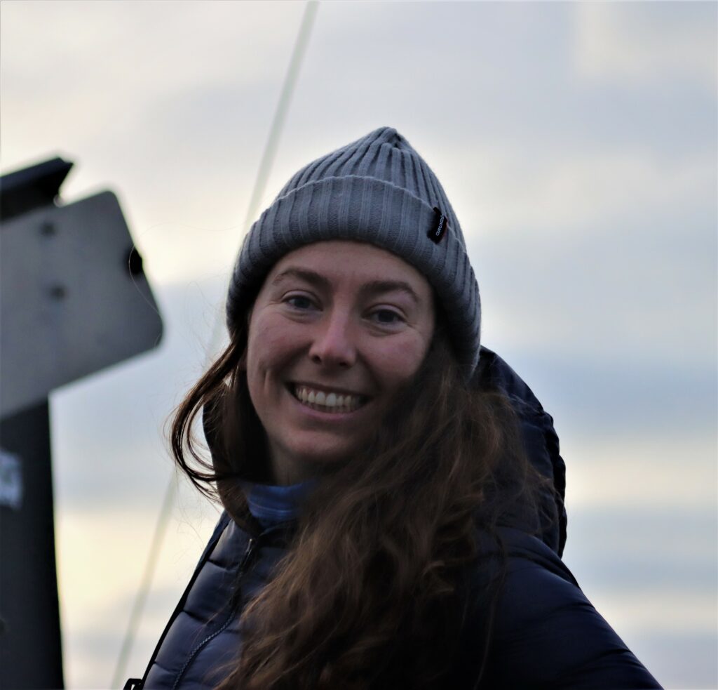
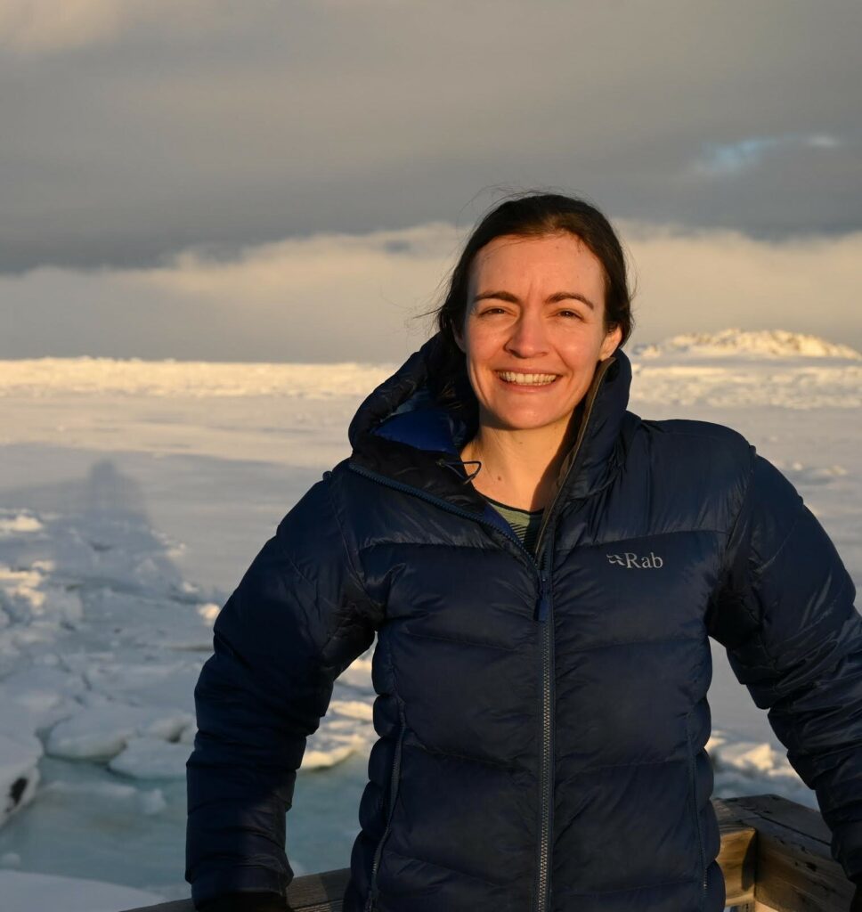
The SAPPHIRE Project is in full swing, as we spend our days aboard the R/V Star Keys searching for krill and blue whales (Figure 1) in the South Taranaki Bight (STB) region of Aotearoa New Zealand. We are investigating how changing ocean conditions impact krill availability and quality, and how this in turn impacts blue whale behavior, health, and reproduction. Understanding the link between changing environmental conditions on prey species and predators is key to understanding the larger implications of climate change on ocean food webs and each populations’ resiliency.

Figure 1. The SAPPHIRE team searching for blue whales. Top left) KC Bierlich, top right) Dawn Barlow, bottom left) Dawn Barlow, Kim Bernard (left to right), bottom right) KC Bierlich, Dawn Barlow, Leigh Torres, Mike Ogle (left to right).

One of the many components of the SAPPHIRE Project is to understand how foraging success of blue whales is influenced by environmental variation (see this recent blog written by Dr. Dawn Barlow introducing each component of the project). When you cannot go to a grocery store or restaurant any time you are hungry, you must rely on stored energy from previous feeds to fuel energy needs. Body condition reflects an individual’s stored energy in the body as a result of feeding and thus represents the foraging success of an individual, which can then affect its potential for reproductive output and the individual’s overall health (see this previous blog). As discussed in a previous blog, drones serve as a valuable tool for obtaining morphological measurements of whales to estimate their body condition. We are using drones to collect aerial imagery of pygmy blue whales to obtain body condition measurements late in the foraging season between years 2024 and 2026 of the SAPPHIRE Project (Figure 2). We are quantifying body condition as Body Area Index (BAI), which is a relative measure standardized by the total length of the whale and well suited for comparing individuals and populations (Figure 3).

The GEMM Lab recently published an article led by Dr. Dawn Barlow where we investigated the differences in BAI between three blue whale populations: Eastern North Pacific blue whales feeding in Monterey Bay, California; Chilean blue whales feeding in the Corcovado Gulf; and New Zealand Pygmy blue whales feeding in the STB (Barlow et al., 2023). These three populations are interesting to compare since blue whales that feed in Monterey Bay and Corcovado Gulf migrate to and from these seasonally productive feeding grounds, while the Pygmy blue whales stay in Aotearoa New Zealand year-round. Interestingly, the Pygmy blue whales had higher BAI (were fatter) compared to the other two regions despite relatively lower productivity in their foraging grounds. This difference in body condition may be due to different life history strategies where the non-migratory Pygmy blue whales may be able to feed as opportunities arrive, while the migratory strategies of the Eastern North Pacific and Chilean blue whales require good timing to access high abundant prey. Another interesting and unexpected result from our blue whale comparison was that Pygmy blue whales are not so “pygmy”; they are actually the same size as Eastern North Pacific and Chilean blue whales, with an average size around 22 m. Our findings from this blue whale comparison leads us to more questions about how environmental conditions that vary from year to year influence body condition and reproduction of these “not so pygmy” blue whales.

Figure 2. An aerial image of a Pygmy blue whale in the South Taranaki Bight region of Aotearoa New Zealand collected during the SAPPHIRE 2024 field season using a DJI Inspire 2 drone.

Figure 3. A drone image of a Pygmy blue whale and the length and body width measurements used to estimate Body Area Index (BAI), represented by the shaded blue region. Width measurements will also be used to help identify pregnant individuals.

The GEMM Lab has been studying this population of Pygmy blue whales in the STB since 2013 and found that years designated as a marine heatwave resulted with a reduction in blue whale feeding activity. Interestingly, breeding activity is also reduced during marine heatwaves in the following season when compared to the breeding season following a more productive, typical foraging season. These findings indicate that fluctuations in the environment, such as marine heatwaves, may affect not only foraging success, but also reproduction in Pygmy blue whales.

To help us better understand reproductive patterns across years, we will use body width measurements from drone images paired with hormone concentrations collected from fecal and biopsy samples to identify pregnant individuals. Progesterone is a hormone secreted in the ovaries of mammals during the estrous cycle and gestation, making it the predominant hormone responsible for sustaining pregnancy. Recently, the GEMM Lab’s Dr. Alejandro Fernandez-Ajo wrote a blog discussing his publication identifying pregnant individual gray whales using drone-based body width measurements and progesterone concentrations from fecal samples (Fernandez et al., 2023). While individuals that were pregnant had higher levels of progesterone compared to when they were not pregnant, the body width at 50% of the body length served as a more reliable method for detecting pregnancy in gray whales. We will use similar methods to help identify pregnancy in Pygmy blue whales for the SAPPHIRE Project where will we examine body width measurement paired with progesterone concentrations collected from fecal and biopsy samples to identify pregnant individuals. We hope our work will help to better understand how climate change will influence Pygmy blue whale body condition and reproduction, and thus the overall health and resiliency of the population. Stay tuned!

References

Barlow, D. R., Bierlich, K. C., Oestreich, W. K., Chiang, G., Durban, J. W., Goldbogen, J. A., Johnston, D. W., Leslie, M. S., Moore, M. J., Ryan, J. P., & Torres, L. G. (2023). Shaped by Their Environment: Variation in Blue Whale Morphology across Three Productive Coastal Ecosystems. Integrative Organismal Biology, 5(1). https://doi.org/10.1093/iob/obad039

Fernandez Ajó, A., Pirotta, E., Bierlich, K. C., Hildebrand, L., Bird, C. N., Hunt, K. E., Buck, C. L., New, L., Dillon, D., & Torres, L. G. (2023). Assessment of a non-invasive approach to pregnancy diagnosis in gray whales through drone-based photogrammetry and faecal hormone analysis. Royal Society Open Science, 10(7), 230452. https://doi.org/10.1098/rsos.230452

It’s getting hot in here: studying the impacts of marine heatwaves on krill, life-blood of the ocean

By Kim Bernard, Associate Professor, Oregon State University College of Earth, Ocean, and Atmospheric Sciences

Euphausiids, commonly known as “krill”, represent a globally distributed family of pelagic crustacean zooplankton, spanning from tropical to polar oceans. These remarkable organisms inhabit a vast range of marine habitats, from nearshore coastal waters to the expansive open ocean, and from the sea surface to abyssal depths. Notably, they claim the title of the largest biomass among non-domestic animal groups on Earth! Beyond their sheer abundance, euphausiids play a pivotal role in shaping global marine food webs, supporting both economically significant fisheries and extensive populations of marine megafauna.

Figure 1: *Nyctiphanes australis*. Photo credit: A. Slotwinski, CSIRO.

As our planet continues to warm, the ongoing and anticipated shifts in the distribution and biomass of krill populations herald potential disruptions to marine ecosystems and food webs globally. Marine heatwaves, which are expected to increase in frequency, intensity, and duration in the coming decades, have a significant impact on global krill populations, with knock-on effects through food webs. At our home-base off the coast of Oregon, a severe marine heatwave in 2014-2016 resulted in altered krill distributions and reduced biomass, causing a suite of ecological implications ranging from decline in salmon health to increased occurrence of whale entanglements in fishing gear (Daly et al. 2017; Santora et al. 2020).

Figure 2: (A) Simrad EK80 transducers (the larger one is a 38kHz transducer, the smaller is a 120kHz transducer) mounted to a pole that gets lowered into the water during our daily surveys. The transducers emit sound waves that bounce off objects, like krill, in the water and return to the instrument’s transceiver, allowing us to map krill within the water column. (B) The acoustic data collected by the echosounder appears in real-time on our computer screen allowing us to find krill that we can then target with the Bongo net. Photo credits: Kim Bernard.

Here, off the coast of New Zealand, the krill species Nyctiphanes australis (Figure 1) is an important prey item for many marine predators, including slender tuna (Allothunnus fallai), Australian salmon (Kahawai, Arripis trutta), Jack mackerel (Trachurus declivis), short-tailed shearwater (Puffinus tenuirostris) (O’Brien 1988), and of course, the reason we are out here, blue whales (Balaenoptera musculus brevicauda) (Torres et al. 2020). In a precursor study to the SAPPHIRE project, members of our current research team demonstrated the potential negative impacts that marine heatwaves can have off the coast of New Zealand. During that study, our team noted declines in the abundance and changes in the distribution patterns of Nyctiphanes australis during a marine heatwave compared to normal conditions, with subsequent negative impacts on the distribution and behavior of the local New Zealand blue whale population (Barlow et al. 2020). The impetus of the SAPPHIRE project is to improve our understanding of the physiological mechanisms underlying the observed changes in both krill and blue whale populations, with the goal to better predict future changes.

As a zooplankton ecologist and “kriller”, my role on the SAPPHIRE project is to further our knowledge on the prey, Nyctiphanes australis. There are several components to this part of our research: (1) mapping distribution patterns of krill, (2) measuring the quality of krill as prey to whales, and (3) running experiments to test how warming affects krill physiology. To map the krill distribution patterns, we are using active acoustics (Figure 2). To measure the quality of krill, we first need to collect them, and we do that using a Bongo net (Figure 3) that gets towed behind the boat targeting krill we find using the echosounder.

Figure 3: Kim Bernard and Ngatokoa Tikitau empty the contents of one of the Bongo net cod-ends into a bucket to examine the catch. Unfortunately, it was not filled with krill as we had hoped, but rather a gelatinous zooplankton known as *Salpa democratica*. Photo credit: KC Bierlich.

Once we have the krill, we’ll flash freeze them in liquid nitrogen and take them back to Oregon where we’ll measure the amount of protein, fats (lipids), and calories each one contains. Finally, for the experiments on temperature effects, we will use live krill collected with the Bongo net placed individually into 1L Nalgene bottles, each outfitted with oxygen sensors so that we can measure the respiration rates of krill at a range of temperatures they would experience during normal conditions and marine heatwaves (Figure 4).

Figure 4: Respiration experiment set-up with two circulating waterbaths in the foreground feeding two temperature treatments in coolers (aka “chilly bins”) behind. Once we catch krill (which has yet to happen), we will use this set-up to test the effects of warming on krill respiration rates. Photo credit: Kim Bernard.

References

Barlow DR, Bernard KS, Escobar-Flores P, Palacios DM, Torres LG (2020) Links in the trophic chain: modeling functional relationships between in situ oceanography, krill, and blue whale distribution under different oceanographic regimes. Marine Ecology Progress Series 642:207-225. https://doi.org/10.3354/meps13339

Daly EA, Brodeur RD, Auth TD (2017) Anomalous ocean conditions in 2015: impacts on spring Chinook salmon and their prey field. Marine Ecology Progress Series 566:169-182. https://doi.org/10.3354/meps12021

O’Brien DP (1988) Surface schooling behaviour of the coastal krill Nyctiphanes australis (Crustacea: Euphausiacea) off Tasmania, Australia. Marine Ecology Progress Series 42: 219-233.

Santora JA, Mantua NJ, Schroeder ID, Field JC, Hazen EL, Bograd SJ, Sydeman WJ, Wells BK, Calambokidis J, Saez L, Lawson D, Forney KA (2020) Habitat compression and ecosystem shifts as potential links between marine heatwave and record whale entanglements. Nature Communications 11(1):536. doi: 10.1038/s41467-019-14215-w.

Torres LG, Barlow DR, Chandler TE, Burnett JD. 2020. Insight into the kinematics of blue whale surface foraging through drone observations and prey data. PeerJ 8:e8906 https://doi.org/10.7717/peerj.8906

Phases and Feelings of the Scientific Journey

Leigh Torres, Associate Professor, PI of the GEMM Lab

There are many phases of a scientific journey, which generally follows a linear path (although I recognize that the process is certainly iterative at times to improve and refine). The scientific journey typically starts with an idea or question, bred from curiosity and passion. The journey hopefully ends with new knowledge, a useful application (e.g., tool or management outcome), and more questions in need of answers, providing a sense of success and pride. But along this path, there are many more phases, with many more emotions. As we begin the four-year SAPPHIRE project, I have already experienced a range of emotions, and I am certain more will come my way as I again wander through the many phases and feeling of science:

PHASE	FEELINGS
Generation of idea or question	Curiosity, passion, wonder
Build the team and develop the funding proposal	Drive, dreaming big, team management, belief in the importance of your proposed work
Notice of funding proposal success	Disbelief, excitement, and pride, followed quickly by feeling daunted, and self-doubt about the ability to pull off what you said you would do.
*Prep for fieldwork/experiment/data collection	Frantic and overwhelmed by the need to remember all the details that make or break the research; lists, lists, lists; pressure to get organized and stay within your budget. Anticipation, exhaustion.
*Outreach/Engagement/Communication	Eagerness to share and connect; Pressure to build relationships and trust; make sure the research is meaningful and accessible to local communities
*Fieldwork/experiment/data collection/data analysis	Sigh of relief to be underway, accompanied by big pressure to achieve: gotta do what you said you would do.
Preparation of scientific publications and reports	Excitement for data synthesis: What will the results say? What are the answers to your burning questions? Were your hypotheses correct? With a good dose of apprehension of peer feedback and critical reviews.
Publications and reports	Satisfaction to see outputs and results from hard work being broadly disseminated.
Project end with final report	Feeling of great accomplishment, but now need to develop the next project and get the funding… the cycle continues.

*After months of intense preparation for our field research component of the SAPPHIRE project in Aotearoa New Zealand (permits, equipment purchasing, community engagement, gathering supplies, learning how to use new equipment, vessel contracting, overseas shipping, travel arrangements, vessel mobilization, oh the list goes on!), we have just stepped off the vessel after 3 full days collecting data. I have cycled through all these emotions many times, and now I feel both exhausted and elated. We are implementing our plan, and we now have data in-hand. Worry creeps in all the time: we need to do more, do better. But I also know that our team is excellent and with patience, blessings from the weather gods, and our continued hard work, we will succeed, learn, and share. As SAPPHIRE chargers ahead to understand the impacts of climate change on marine prey (krill) and predators (blue whales), I am ready for the continued mix of emotions that comes with science.

Photo montage of our awesome SAPPHIRE team in prep mode and during data collection in the South Taranaki Bight within Aotearoa New Zealand.

Blue whales, krill, and climate change: introducing the SAPPHIRE project

By Dr. Dawn Barlow, Postdoctoral Scholar, OSU Department of Fisheries, Wildlife, and Conservation Sciences, Geospatial Ecology of Marine Megafauna Lab

The world is warming. Ocean ecosystems are experiencing significant and rapid impacts of climate change. However, the cascading effects on marine life are largely unknown. Thus, it is critical to understand how – not just if – environmental change impacts the availability and quality of key prey species in ocean food webs, and how these changes will impact marine predator health and population resilience. With these pressing knowledge gaps in mind, we are thrilled to launch a new project “Marine predator and prey response to climate change: Synthesis of Acoustics, Physiology, Prey, and Habitat in a Rapidly changing Environment (SAPPHIRE).” We will examine how changing ocean conditions affect the availability and quality of krill, and thus impact blue whale behavior, health, and reproduction. This large-scale research effort is made possible with funding from the National Science Foundation.

The SAPPHIRE project takes place in the South Taranaki Bight (STB) region of Aotearoa New Zealand, and before diving into our new research plans, let’s reflect briefly on what we know so far about this study system based on our previous research. Our collaborative research team has studied blue whales in the STB since 2013 to document the population, understand their ecology and habitat use, and inform conservation management. We conducted boat-based surveys and used hydrophones to record the underwater soundscape, and found the following:

Blue whales in Aotearoa New Zealand are a unique population, genetically distinct from all other known populations in the Southern Hemisphere, with an estimated population size of 718 (95% CI = 279 – 1926).¹
Blue whales reside in the STB region year-round, with feeding and breeding vocalizations detected nearly every day of the year.^2,3
Wind-driven upwelling over Kahurangi shoals moves a plume of cold, nutrient-rich waters into the STB, supporting aggregations of krill, and thereby critical feeding opportunities for blue whales in spring and summer.^4–6
We developed predictive models to forecast blue whale distribution up to three weeks in advance, providing managers with a real-time tool in the form of a desktop application to produce daily forecast maps for dynamic management.⁷
During marine heatwaves, blue whale feeding activity was substantially reduced in the STB. Interestingly, their breeding activity was also reduced in the following season when compared to the breeding season following a more productive, typical foraging season. This finding indicates that shifting environmental conditions, such as marine heatwaves and climate change, may have consequences to not just foraging success, but the population’s reproductive patterns.³

A blue whale comes up for air in the South Taranaki Bight. Photo by Leigh Torres.

Project goals

Building on this existing knowledge, we aim to gain understanding of the health impacts of environmental change on krill and blue whales, which can in turn inform management decisions. Over the next three years (2024-2026) we will use multidisciplinary methods to collect data in the field that will enable us to tackle these important but challenging goals. Our broad objectives are to:

Assess variation in krill quality and availability relative to rising temperatures and different ocean conditions,
Document how blue whale body condition and hormone profiles change relative to variable environmental and prey conditions,
Understand how environmental conditions impact blue whale foraging and reproductive behavior, and
Integrate these components to develop novel Species Health Models to predict predator and prey whale population response to rapid environmental change.

Kicking off fieldwork

This coming January, we will set sail aboard the R/V Star Keys and head out in search of blue whales and krill in the STB! Five of our team members will spend three weeks at sea, during which time we will conduct surveys for blue whale occurrence paired with active acoustic assessment of krill availability, fly Unoccupied Aircraft Systems (UAS; “drones”) over whales to determine body condition and potential pregnancy, collect tissue biopsy samples to quantify stress and reproductive hormone levels, deploy hydrophones to record rates of foraging and reproductive calls by blue whales, and conduct on-board controlled experiments on krill to assess their response to elevated temperature.

The team in action aboard the R/V Star Keys in February 2017. Photo by L. Torres.

The moving pieces are many as we work to obtain research permits, engage in important consultation with iwi (indigenous Māori groups), procure specialized scientific equipment, and make travel and shipping arrangements. The to-do lists seem to grow just as fast as we can check items off; such is the nature of coordinating an international, multidisciplinary field effort. But it will pay off when we are underway, and I can barely contain my excitement to back on the water with this research team.

Our team has not collected data in the STB since 2017. We know so much more now than we did when studies of this blue whale population were just beginning. For example, we are eager to put our blue whale forecast tool to use, which will hopefully enable us to direct survey effort toward areas of higher blue whale density to maximize data collection. We are keen to see what new insights we gain, and what new questions and challenges arise.

Research team

The SAPPHIRE project will only be possible with the expertise and coordination of the many members of our collaborative group. We are all thrilled to begin this research journey together, and eager to share what we learn.

Principal Investigators:

Leigh Torres (Geospatial Ecology of Marine Megafauna Lab, Marine Mammal Institute, OSU)

Research partners and key collaborators:

References:

1. Barlow DR, Torres LG, Hodge KB, Steel D, Baker CS, Chandler TE, Bott N, Constantine R, Double MC, Gill P, Glasgow D, Hamner RM, Lilley C, Ogle M, Olson PA, Peters C, Stockin KA, Tessaglia-Hymes CT, Klinck H. Documentation of a New Zealand blue whale population based on multiple lines of evidence. Endanger Species Res. 2018;36:27–40.

2. Barlow DR, Klinck H, Ponirakis D, Holt Colberg M, Torres LG. Temporal occurrence of three blue whale populations in New Zealand waters from passive acoustic monitoring. J Mammal. 2022;

3. Barlow DR, Klinck H, Ponirakis D, Branch TA, Torres LG. Environmental conditions and marine heatwaves influence blue whale foraging and reproductive effort. Ecol Evol. 2023;13:e9770.

4. Barlow DR, Klinck H, Ponirakis D, Garvey C, Torres LG. Temporal and spatial lags between wind, coastal upwelling, and blue whale occurrence. Sci Rep. 2021;11(6915):1–10.

5. Barlow DR, Bernard KS, Escobar-Flores P, Palacios DM, Torres LG. Links in the trophic chain: Modeling functional relationships between in situ oceanography, krill, and blue whale distribution under different oceanographic regimes. Mar Ecol Prog Ser. 2020;642:207–25.

6. Torres LG, Barlow DR, Chandler TE, Burnett JD. Insight into the kinematics of blue whale surface foraging through drone observations and prey data. PeerJ. 2020;8:e8906.

7. Barlow DR, Torres LG. Planning ahead: Dynamic models forecast blue whale distribution with applications for spatial management. J Appl Ecol. 2021;58(11):2493–504.

New GEMM Lab publication reveals how blue whale feeding and reproductive effort are related to environmental conditions

By Dr. Dawn Barlow, Postdoctoral Scholar, OSU Department of Fisheries, Wildlife, and Conservation Sciences, Geospatial Ecology of Marine Megafauna Lab

Learning by listening

Studying mobile marine animals that are only fleetingly visible from the water’s surface is challenging. However, many species including baleen whales rely on sound as a primary form of communication, producing different vocalizations related to their fundamental needs to feed and reproduce. Therefore, we can learn a lot about these elusive animals by monitoring the patterns of their calls. In the final chapter of my PhD, we set out to study blue whale ecology and life history by listening. I am excited to share our findings, recently published in Ecology and Evolution.

Blue whales produce two distinct types of vocalizations: song is produced by males and is hypothesized to play a role in breeding behavior, and D calls are a hypothesized social call produced by both sexes in association with feeding behavior. We analyzed how these different calls varied seasonally, and how they related to environmental conditions.

This paper is a collaborative study co-authored by Dr. Holger Klinck and Dimitri Ponirakis of the K. Lisa Yang Center for Conservation Bioacoustics, Dr. Trevor Branch of the University of Washington, and GEMM Lab PI Dr. Leigh Torres, and brings together multiple methods and data sources. Our findings shed light on blue whale habitat use patterns, and how climate change may impact both feeding and reproduction for this species of conservation concern.

The South Taranaki Bight: an ideal study system

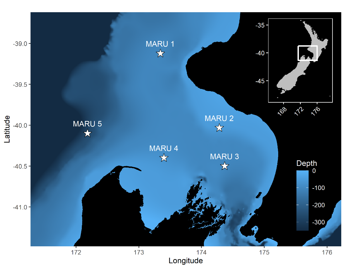
Baleen whales typically migrate between high-latitude, productive feeding grounds and low-latitude breeding grounds. However, the New Zealand blue whale population is present in the South Taranaki Bight (STB) region year-round, which uniquely enabled us to monitor their behavior, ecology, and life history across seasons and years from a single location. We recorded blue whale vocalizations from Marine Autonomous Recording Units (MARUs) deployed at five locations in the STB for two full years (Fig. 1).

Figure 1. Study area map and blue whale call spectrograms. Left panel: map of the study area in the South Taranaki Bight region, with hydrophone (marine autonomous recording unit; MARU) locations denoted by the stars. Gray lines show bathymetry contours at 50 m depth increments, from 0 to 500 m. Location of the study area within New Zealand is indicated by the inset map. Right panels: example spectrograms of the two blue whale call types examined: the New Zealand song recorded on 31 May 2016 (top) and D calls recorded 20 September 2016 (bottom). Figure reproduced from Barlow et al. (2023).

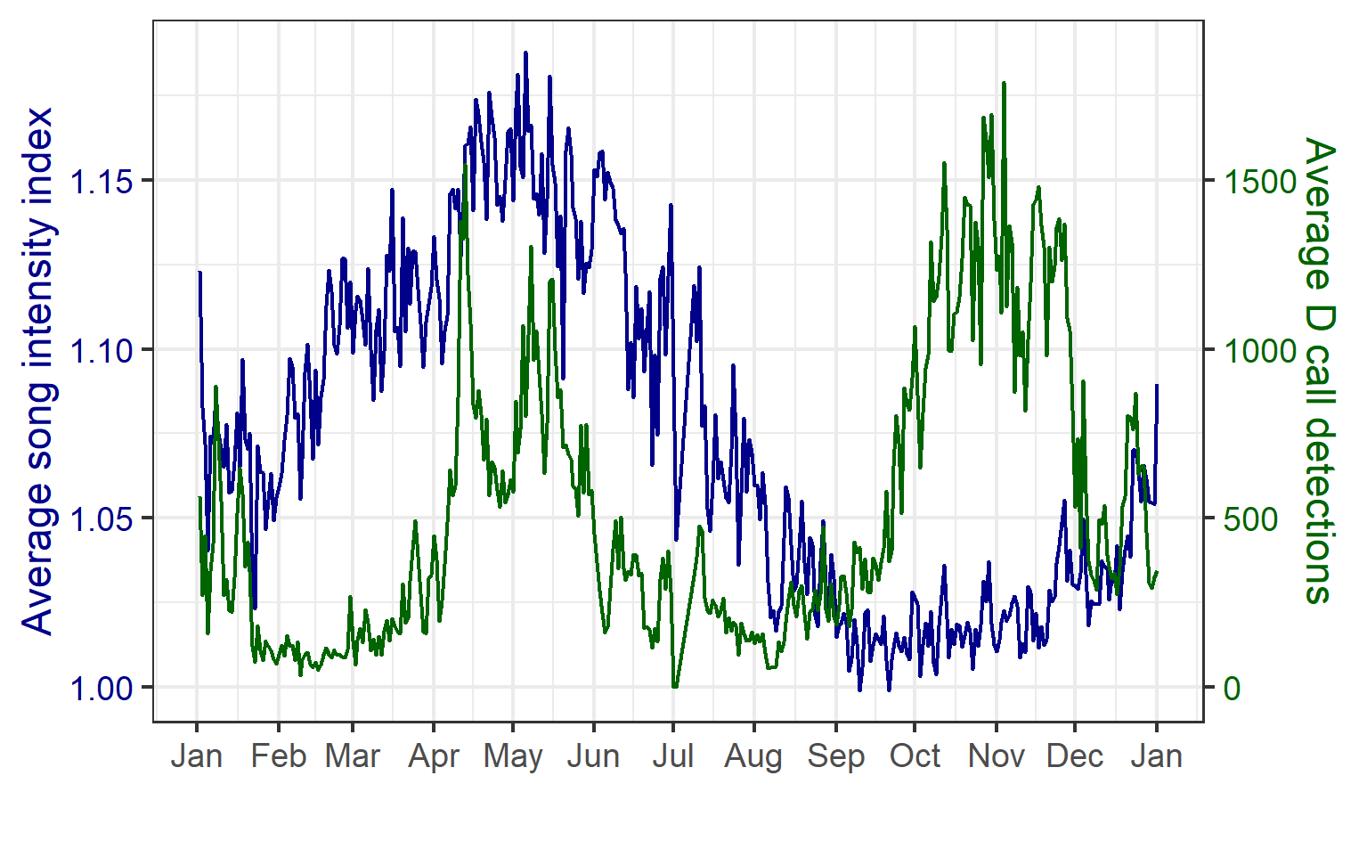
We found that the two vocalization types had different seasonal occurrence patterns (Fig. 2). D calls were associated with upwelling conditions that indicate feeding opportunities, lending evidence for their function as a foraging-related call.

Figure 2. Average annual cycle in the song intensity index (dark blue) and D calls (green) per day of the year, computed across all hydrophone locations and the entire two-year recording period. Figure reproduced from Barlow et al. (2023).

In contrast, blue whale song showed a very clear seasonal peak in the fall and was less obviously correlated with environmental conditions. To investigate the hypothesized function of song as a breeding call, we turned to a perhaps unintuitive source of information: historical whaling records. Whenever a pregnant whale was killed during commercial whaling operations, the length of the fetus was measured. By looking at the seasonal pattern in these fetal lengths, we can presume that births occur around the time of year when fetal lengths are at their longest. The records indicated April-May. By back-calculating the 11-month gestation time for a blue whale, we can presume that mating occurs generally in May-June, which is the exact time of the peak in song intensity from our recordings (Fig. 3).

Figure 3. Annual song intensity and the breeding cycle. Top panel: average yearly cycle in song intensity index, computed across the five hydrophone locations and the entire recording period; dark blue line represents a loess smoothed fit. Bottom panel: fetal length measurements from whaling catch records for Antarctic blue whales (gray, measurements rounded to the nearest foot), pygmy blue whales in the southern hemisphere (blue, measurements rounded to the nearest centimeter). Measurements from blue whales caught within the established range of the New Zealand population are denoted by the dark red triangles. Calving presumably takes place around or shortly after fetal lengths are at their maximum (April–May), which implies that mating likely occurs around May–June, coincident with the peak song intensity. Figure reproduced from Barlow et al. (2023).

With this evidence for D calls as feeding-related calls and song as breeding-related calls, we had a host of new questions, we used this gained knowledge to explore how changing environmental conditions might impact multiple life history processes for New Zealand blue whales

Marine heatwaves impact multiple life history processes

Our study period between January 2016 and February 2018 spanned both typical upwelling conditions and dramatic marine heatwaves in the STB region. While we previously documented that the marine heatwave of 2016 affected blue whale distribution, the population-level impacts on feeding and reproductive effort remained unknown. In our recent study, we found that during marine heatwaves, D calls were dramatically reduced compared to during productive upwelling conditions. During the fall breeding peak, song intensity was likewise dramatically reduced following the marine heatwave. This relationship indicates that following poor feeding conditions, blue whales may invest less effort in reproduction. As marine heatwaves are projected to become more frequent and more intense under global climate change, our findings are perhaps a warning for what is to come as animal populations must contend with changing ocean conditions.

More than a decade of research on New Zealand blue whales

Ten years ago, Leigh first put forward a hypothesis that the STB region was an undocumented blue whale foraging ground based on multiple lines of evidence (Torres 2013). Despite pushback and numerous challenges, Leigh set out to prove her hypothesis through a comprehensive, multi-year data collection effort. I was lucky enough to join the team in 2016, first as a Masters’ student, and then as a PhD student. In the time since Leigh’s hypothesis, we not only documented the New Zealand blue whale population (Barlow et al. 2018), we learned a great deal about what drives blue whale feeding behavior (Torres et al. 2020) and habitat use patterns (Barlow et al. 2020, 2021), and developed forecast models to predict blue whale distribution for dynamic management of the STB (Barlow & Torres 2021). We also documented their unique, year-round presence in the STB, distinct from the migratory or vagrant presence of other blue whale populations (Barlow et al. 2022b). We now understand how marine heatwaves impact both feeding opportunities and reproductive effort (Barlow et al. 2023). We even analyzed blue whale skin condition (Barlow et al. 2019) and acoustic response to earthquakes (Barlow et al. 2022a) along the way. A decade later, it is humbling to reflect on how much we have learned about these whales. This paper is also the final chapter of my PhD, and as I reflect on how I have grown both personally and scientifically since I interviewed with Leigh as a wide-eyed undergraduate student in fall 2015, I am filled with gratitude for the opportunities for learning and growth that Leigh, these whales, and many mentors and collaborators have offered over the years. As is often the case in science, the more questions you ask, the more questions you end up with. We are already dreaming up future studies to further understand the ecology, health, and resilience of this blue whale population. I can only imagine what we might learn in another decade.

Figure 5. A blue whale mother and calf pair come up for air in the South Taranaki Bight. Photo by Dawn Barlow.

References:

Barlow DR, Bernard KS, Escobar-Flores P, Palacios DM, Torres LG (2020) Links in the trophic chain: Modeling functional relationships between in situ oceanography, krill, and blue whale distribution under different oceanographic regimes. Mar Ecol Prog Ser 642:207–225.

Barlow DR, Estrada Jorge M, Klinck H, Torres LG (2022a) Shaken, not stirred: blue whales show no acoustic response to earthquake events. R Soc Open Sci 9:220242.

Barlow DR, Klinck H, Ponirakis D, Branch TA, Torres LG (2023) Environmental conditions and marine heatwaves influence blue whale foraging and reproductive effort. Ecol Evol 13:e9770.

Barlow DR, Klinck H, Ponirakis D, Garvey C, Torres LG (2021) Temporal and spatial lags between wind, coastal upwelling, and blue whale occurrence. Sci Rep 11:1–10.

Barlow DR, Klinck H, Ponirakis D, Holt Colberg M, Torres LG (2022b) Temporal occurrence of three blue whale populations in New Zealand waters from passive acoustic monitoring. J Mammal.

Barlow DR, Pepper AL, Torres LG (2019) Skin deep: An assessment of New Zealand blue whale skin condition. Front Mar Sci 6:757.

Barlow DR, Torres LG (2021) Planning ahead: Dynamic models forecast blue whale distribution with applications for spatial management. J Appl Ecol 58:2493–2504.

Barlow DR, Torres LG, Hodge KB, Steel D, Baker CS, Chandler TE, Bott N, Constantine R, Double MC, Gill P, Glasgow D, Hamner RM, Lilley C, Ogle M, Olson PA, Peters C, Stockin KA, Tessaglia-hymes CT, Klinck H (2018) Documentation of a New Zealand blue whale population based on multiple lines of evidence. Endanger Species Res 36:27–40.

Torres LG (2013) Evidence for an unrecognised blue whale foraging ground in New Zealand. New Zeal J Mar Freshw Res 47:235–248.

Torres LG, Barlow DR, Chandler TE, Burnett JD (2020) Insight into the kinematics of blue whale surface foraging through drone observations and prey data. PeerJ 8:e8906.

The many dimensions of a fat whale: Using drones to measure the body condition of baleen whales

Dr. KC Bierlich, Postdoctoral Scholar, OSU Department of Fisheries, Wildlife, & Conservation Sciences, Geospatial Ecology of Marine Megafauna (GEMM) Lab

In my last blog, I discussed how to obtain morphological measurements from drone-based imagery of whales and the importance of calculating and considering uncertainty, as different drone platforms have varying levels of measurement uncertainty. But how does uncertainty scale and propagate when multiple measurements are combined, such as when measuring body condition of the whole animal? In this blog, I will discuss the different methods used for measuring body condition of baleen whales from drone-based imagery and how uncertainty differs between these metrics.

Body condition is defined as the energy stored in the body as a result of feeding and is assumed to indicate an animal’s overall health, as it reflects the balance between energy intake and investment toward growth, maintenance and reproduction (Peig and Green, 2009). Thus, body condition reflects the foraging success of an individual, as well as the potential for reproductive output and the quality of habitat. For example, female North American brown bears (Ursus arctos) in high quality habitats were in better body condition, produced larger litter sizes, and lived in greater population densities compared to females in lower quality habitats (Hilderbrand et al., 1999). As Dawn Barlow and Will Kennerley discussed in their recent blog, baleen whales are top predators and serve as ecosystem sentinels that shed light not only on the health of their population, but on the health of their ecosystem. As ocean climate conditions continue to change, monitoring the body condition of baleen whales is important to provide insight on how their population and ecosystem is responding.

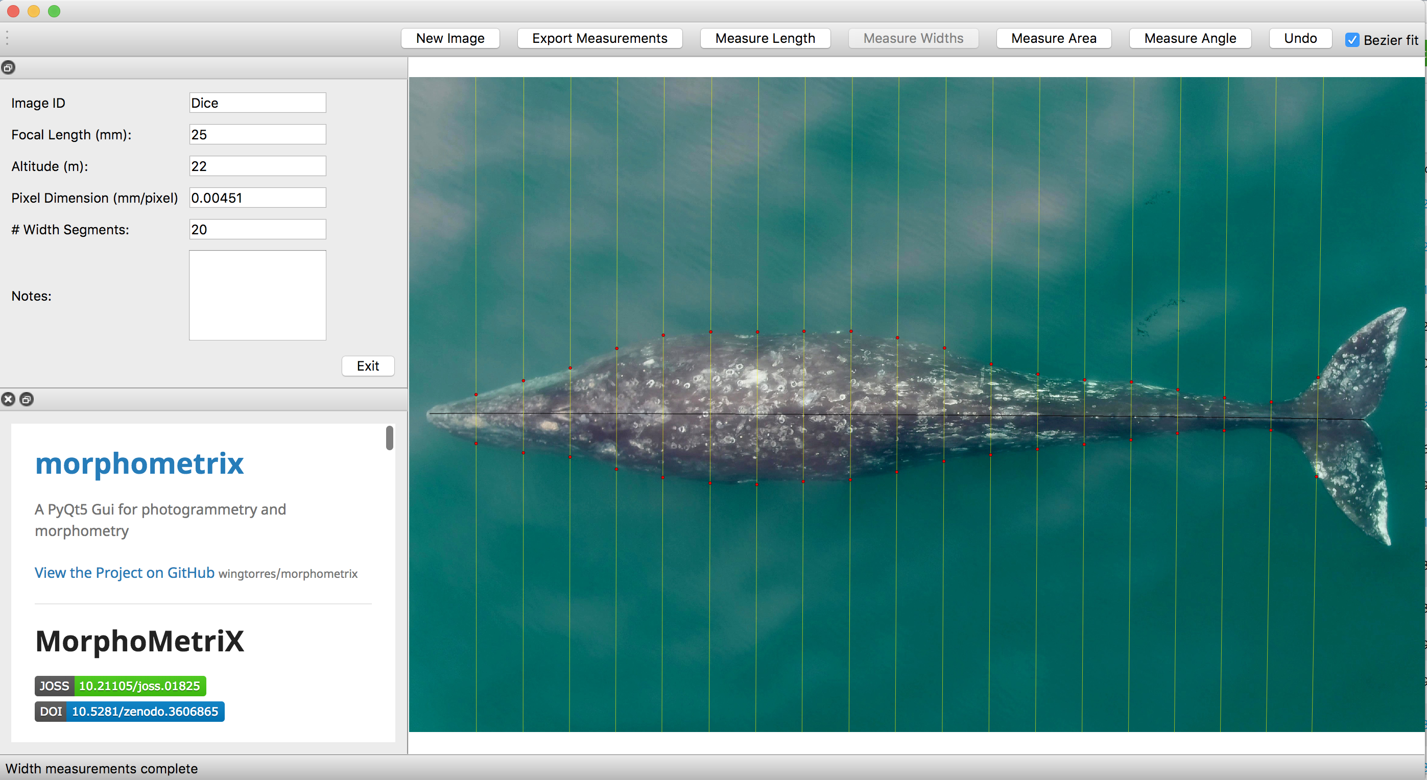
As discussed in a previous blog, drones serve as a valuable tool for obtaining morphological measurements of baleen whales to estimate their body condition. Images are imported into photogrammetry software, such as MorphoMetriX (Torres and Bierlich, 2020), to measure the total length of an individual and that is then divided into perpendicular width segments (i.e., in 5 or 10% increments) down the body (Fig. 1). These total length and width measurements are then used to estimate body condition in either 1-, 2-, or 3-dimensions: a single width (1D), a projected dorsal surface area (2D), or a body volume measure (3D). These 1D, 2D, and 3D measurements of body condition can then be standardized by total length to produce a relative measure of an individual’s body condition to compare among individuals and populations.

Figure 1. An example of a Pacific Coast Feeding Group (PCFG) gray whale measured in MorphoMetriX (Torres & Bierlich, 2020).

While several different studies have used each of these dimensions to assess whale body condition, it is unclear how these measurements compare amongst each other. Importantly, it is also unclear how measurement uncertainty scales across these multiple dimensions and influences inference, which can lead to misinterpretation of data. For example, the surface area and volume of two geometrically similar bodies of different sizes are not related to their linear dimensions in the same ratio, but rather to the second and third power, respectively (i.e., x² vs. x³). Similarly, uncertainty should not be expected to scale linearly across 1D, 2D, and 3D body condition measurements.

The second chapter of my dissertation, which was recently published in Frontiers in Marine Science and includes Clara Bird and Leigh Torres as co-authors, compared the uncertainty associated with 1D, 2D, and 3D drone-based body condition measurements in three baleen whale species with different ranges in body sizes: blue, humpback, and Antarctic minke whales (Figure 2) (Bierlich et al., 2021). We used the same Bayesian model discussed in my last blog, to incorporate uncertainty associated with each 1D, 2D, and 3D estimate of body condition.

Figure 2. An example of total length and perpendicular width (in 5% increments of total length) measurements of an individual blue, humpback and Antarctic minke whale. Each image measured using MorphoMetriX (Torres and Bierlich, 2020).

We found that uncertainty does not scale linearly across multi-dimensional measurements, with 2D and 3D uncertainty increasing by a factor of 1.45 and 1.76 compared to 1D, respectively. This result means that there is an added cost of increased uncertainty when utilizing a multidimensional body condition measurement. Our finding is important to help researchers decide which body condition measurement best suits their scientific question, particularly when using a drone platform that is susceptible to greater error – as discussed in my previous blog. However, a 1D measurement only relies on a single width measurement, which may be excluding other regions of an individual’s body condition that is important for energy storage. In these situations, a 2D or 3D measure may be more appropriate.

We found that when comparing relative measures of body condition (standardized by total length of the individual), each standardized metric was highly correlated with one another. This finding suggests that 1D, 2D, and 3D metrics will draw similar relative predictions of body condition for individuals, allowing researchers to be confident they will draw similar conclusions relating to the body condition of individuals, regardless of which standardized metric they use. However, when comparing the precision of each of these metrics, the body area index (BAI) – a 2D standardized metric – displayed the highest level of precision. This result highlights how BAI can advantageously detect small changes in body condition, which is useful for comparing individuals or even tracking the same individual over time.

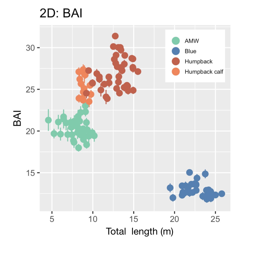
BAI was developed by the GEMM Lab (Burnett et al., 2018) and was designed to be similar to body mass index (BMI) in humans [BMI = mass (kg)/(height (m))²], where BAI uses the calculated surface area as a surrogate for body mass. In humans, a healthy BMI range is generally considered 18.5–24.9, below 18.5 is considered underweight, above 24.9 is considered overweight, and above 30 is considered obese (Flegal et al., 2012). Identifying a healthy range in BAI for baleen whales is challenged by a limited knowledge of what a “healthy” body condition range is for a whale. We found strong evidence that a healthy range of BAI is species-specific, as each species displayed a distinctive range in BAI: blue whales: 11–16; AMW: 17–24; humpback whales: 23–32; humpback whale calves: 23–28 (Fig. 3). These differences in BAI ranges likely reflect differences in the body shape of each species (Fig. 4). For example, humpbacks have the widest range of BAI compared to these other two species, which was also reflected in their larger variation in perpendicular widths (Figs. 2-4). Thus, it seems that BAI offers conditionally “scalefree” comparisons between species, yet it is unreasonable to set a single, all-whale BAI threshold to determine “healthy” versus “unhealthy” body condition. Collecting a large sample of body condition measurements across many individuals and demographic units over space and time with information on vital rates (e.g., reproductive capacity) will help elucidate a healthy BAI range for each species.

Figure 3. Body area index (BAI) for each species. AMW = Antarctic minke whale. Figure from Bierlich et al. (2021).

Figure 4. A) Absolute widths (m) and B) relative widths, standardized by total length (TL) to help elucidate the different body shapes of Antarctic minke whales (AMW; n = 40), blue whales (n = 32), humpback whales (n = 40), and humpback whale calves (n = 15). Note how the peak in body width occurs at a different percent body width between species, demonstrating the natural variation in body shape between baleen whales. Figure from Bierlich et al. (2021).

Over the past six years, the GEMM Lab has been collecting drone images of Pacific Coast Feeding Group (PCFG) gray whales off the coast of Oregon to measure their BAI (see GRANITE Project blog). Many of the individuals we encounter are seen across years and throughout the foraging season, providing an opportunity to evaluate how an individual’s BAI is influenced by environmental variation, stress levels, maturity, and reproduction. These data will in turn help determine what the healthy range in BAI for gray whales is. For example, linking BAI to pregnancy – whether a whale is currently pregnant or becomes pregnant the following season – will help determine what BAI is needed to support calf production. We are currently analyzing hundreds of body condition measurements from 2016 – 2021, so stay tuned for upcoming results!

References

Bierlich, K. C., Hewitt, J., Bird, C. N., Schick, R. S., Friedlaender, A., Torres, L. G., … & Johnston, D. W. (2021). Comparing Uncertainty Associated With 1-, 2-, and 3D Aerial Photogrammetry-Based Body Condition Measurements of Baleen Whales. Frontiers in Marine Science, 1729.

Burnett, J. D., Lemos, L., Barlow, D., Wing, M. G., Chandler, T., & Torres, L. G. (2018). Estimating morphometric attributes of baleen whales with photogrammetry from small UASs: A case study with blue and gray whales. Marine Mammal Science, 35(1), 108–139.

Flegal, K. M., Carroll, M. D., Kit, B. K., & Ogden, C. L. (2012). Prevalence of Obesity and Trends in the Distribution of Body Mass Index Among US Adults, 1999-2010. JAMA, 307(5), 491. https://doi.org/10.1001/jama.2012.39

Hilderbrand, G. V, Schwartz, C. C., Robbins, C. T., Jacoby, M. E., Hanley, T. A., Arthur, S. M., & Servheen, C. (1999). The importance of meat, particularly salmon, to body size, population productivity, and conservation of North American brown bears. Canadian Journal of Zoology, 77(1), 132–138.

Peig, J., & Green, A. J. (2009). New perspectives for estimating body condition from mass/length data: the scaled mass index as an alternative method. Oikos, 118(12), 1883–1891.

Torres, W., & Bierlich, K. C. (2020). MorphoMetriX: a photogrammetric measurement GUI for morphometric analysis of megafauna. Journal of Open Source Software, 5(45), 1825–1826.

Different blue whale populations sing different songs

By Dawn Barlow, PhD Candidate, OSU Department of Fisheries, Wildlife, and Conservation Sciences, Geospatial Ecology of Marine Megafauna Lab

In human cultures, how you sound is often an indicator of where you are from. Have you ever taken a linguistics quiz that tries to guess what part of the United States you grew up in? Questions about whether you pronounce the sugary sweet treat caramel as “carr-mul” or “care-a-mel”, whether you say “soda” or “pop”, or whether a certain type of intersection is called a “roundabout”, “rotary”, or “traffic circle” are used to make a guess at where in the country you were raised. I have spent time in the United States, Australia, and New Zealand, I was amused to learn that the shoes you might wear in summertime can be called flip flops, slippers, thongs, or jandals, depending on which English-speaking country you are in. We know that listening to how someone speaks can tell us about their heritage or culture. As it turns out, the same is true for blue whales. We can learn a lot about blue whales by listening to them.

A blue whale comes up for air in the South Taranaki Bight, New Zealand. We catch only a short glimpse of these ocean giants when they are at the surface. By listening to their vocalizations using acoustic recordings, we can gain a whole new perspective on their lives. Photo by D. Barlow.

Sound is an incredibly important sense to marine mammals, particularly since sound waves can efficiently transmit over long distances in the ocean where other senses, such as vision or smell, are limited. Therefore, passive acoustic monitoring—placing hydrophones underwater to listen for an extended period of time and record the sounds of animals and their environment—is a highly effective tool for studying marine mammals, including blue whales. Throughout the world, blue whales sing. In this case, “song” is defined as a limited number of sound types that are produced in succession to form a recognizable pattern (McDonald et al. 2006). These songs are presumed to be produced by males only, most likely used to maintain associations and mediate social interactions, and seem to play a role in reproduction (Oleson et al. 2007, Lewis et al. 2018). Furthermore, these songs are highly stereotyped, and stable over decadal scales (McDonald et al. 2006).

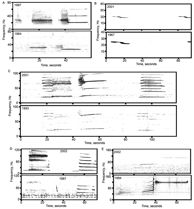
Figure reproduced from McDonald et al. (2006), illustrating the variation and in blue whale songs from different geographic regions, and their stability over time: Recordings from New Zealand (A), the Central North Pacific (B), Australia (C), the Northeast Pacific (D) and North Indian Ocean (E) illustrate the stable character of the blue whale song over long time periods. All song types for which long time spans of recordings are available show some frequency drift through time, but only minor change in character. These examples were chosen because recordings over a significant time span were available to the authors in raw form, and not because these song types are more stable than the others.

Fascinatingly, blue whale songs have acoustic characteristics that are distinct between geographic regions. A blue whale in the northeast Pacific sings a different song than a blue whale in the north Atlantic; the song heard around Australia is distinct from the one sung off the coast of Chile, and so on. Therefore, differences in blue whale songs between areas can be used as a provisional hypothesis about population structure (McDonald et al. 2006, Samaran et al. 2013, Balcazar et al. 2015). Vocalizations may evolve more rapidly than traditional markers such as genetics or morphology that are often used to delineate populations, particularly in long-lived mammalian species such as blue whales (McDonald et al. 2006).

Figure reproduced from McDonald et al. (2006): Blue whale residence and population divisions suggested from their song types. Arrows indicate the direction of seasonal movements.

Despite the general rule of thumb that population-specific blue whale songs occur in separate geographic regions, there are examples throughout the southern hemisphere where songs from different populations overlap and are recorded in the same location (Samaran et al. 2010, 2013, Tripovich et al. 2015, McCauley et al. 2018, Buchan et al. 2020, Leroy et al. 2021). However, these examples may be instances where the populations temporally or ecologically partition their use of the area. For example, there may be differences in the timing of peak occurrence so that overlap is minimized by alternating which population is predominantly present in different seasons (Leroy et al. 2018). Alternatively, whales from different populations may overlap in space and time, but occupy different ecological niches at the same site. In this case, an area may simultaneously be a migratory corridor for one population and a foraging ground for another (Tripovich et al. 2015).

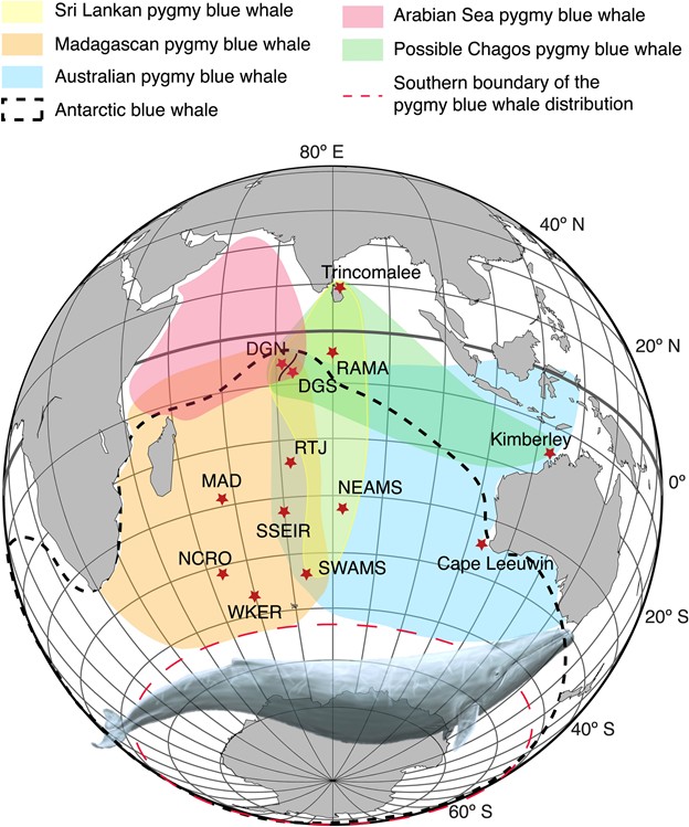
Figure reproduced from Leroy et al. (2021): Distribution of the five blue whale acoustic populations of the Indian Ocean: the Sri Lankan—NIO (yellow); Madagascan—SWIO (orange); Australian—SEIO (blue); and Arabian Sea—NWIO (red) pygmy blue whales; the hypothesized Chagos pygmy blue whale (green); and the Antarctic blue whale (black dashed line). These distributions have been inferred from the acoustic recordings conducted in the area. The long-term recording sites used to infer these distribution areas are indicated by red stars. Blue whale illustration by Alicia Guerrero.

In the South Taranaki Bight (STB) region of New Zealand, where the GEMM lab has been studying blue whales for the past decade (Torres 2013), the New Zealand song type is recorded year-round (Barlow et al. 2018). New Zealand blue whales rely on a productive upwelling system in the STB that supports an important foraging ground (Barlow et al. 2020, 2021). Antarctic blue whales also seasonally pass through New Zealand waters, likely along their migratory pathway between polar feeding grounds and lower latitude areas (Warren et al. 2021). What does it mean in terms of population connectivity or separation when two different populations occasionally share the same waters? How do these different populations ecologically partition the space they occupy? What drives their differing occurrence patterns? These are the sorts of questions I am diving into as we continue to explore the depths of our acoustic recordings from the STB region. We still have a lot to learn about these blue whales, and there is a lot to be learned through listening.

References:

Balcazar NE, Tripovich JS, Klinck H, Nieukirk SL, Mellinger DK, Dziak RP, Rogers TL (2015) Calls reveal population structure of blue whales across the Southeast Indian Ocean and the Southwest Pacific Ocean. J Mammal 96:1184–1193.

Barlow DR, Klinck H, Ponirakis D, Garvey C, Torres LG (2021) Temporal and spatial lags between wind, coastal upwelling, and blue whale occurrence. Sci Rep 11:1–10.

Buchan SJ, Balcazar-Cabrera N, Stafford KM (2020) Seasonal acoustic presence of blue, fin, and minke whales off the Juan Fernández Archipelago, Chile (2007–2016). Mar Biodivers 50:1–10.

Leroy EC, Royer JY, Alling A, Maslen B, Rogers TL (2021) Multiple pygmy blue whale acoustic populations in the Indian Ocean: whale song identifies a possible new population. Sci Rep 11:8762.

Leroy EC, Samaran F, Stafford KM, Bonnel J, Royer JY (2018) Broad-scale study of the seasonal and geographic occurrence of blue and fin whales in the Southern Indian Ocean. Endanger Species Res 37:289–300.

Lewis LA, Calambokidis J, Stimpert AK, Fahlbusch J, Friedlaender AS, Mckenna MF, Mesnick SL, Oleson EM, Southall BL, Szesciorka AR, Širović A (2018) Context-dependent variability in blue whale acoustic behaviour. R Soc Open Sci 5.

McCauley RD, Gavrilov AN, Jolli CD, Ward R, Gill PC (2018) Pygmy blue and Antarctic blue whale presence , distribution and population parameters in southern Australia based on passive acoustics. Deep Res Part II 158:154–168.

McDonald MA, Mesnick SL, Hildebrand JA (2006) Biogeographic characterisation of blue whale song worldwide: using song to identify populations. J Cetacean Res Manag 8:55–65.

Oleson EM, Wiggins SM, Hildebrand JA (2007) Temporal separation of blue whale call types on a southern California feeding ground. Anim Behav 74:881–894.

Samaran F, Adam O, Guinet C (2010) Discovery of a mid-latitude sympatric area for two Southern Hemisphere blue whale subspecies. Endanger Species Res 12:157–165.

Samaran F, Stafford KM, Branch TA, Gedamke J, Royer J, Dziak RP, Guinet C (2013) Seasonal and Geographic Variation of Southern Blue Whale Subspecies in the Indian Ocean. PLoS One 8:e71561.

Torres LG (2013) Evidence for an unrecognised blue whale foraging ground in New Zealand. New Zeal J Mar Freshw Res 47:235–248.

Tripovich JS, Klinck H, Nieukirk SL, Adams T, Mellinger DK, Balcazar NE, Klinck K, Hall EJS, Rogers TL (2015) Temporal Segregation of the Australian and Antarctic Blue Whale Call Types (Balaenoptera musculus spp.). J Mammal 96:603–610.

Warren VE, Širović A, McPherson C, Goetz KT, Radford CA, Constantine R (2021) Passive Acoustic Monitoring Reveals Spatio-Temporal Distributions of Antarctic and Pygmy Blue Whales Around Central New Zealand. Front Mar Sci 7:1–14.

Supporting marine life conservation as an outsider: Blue whales and earthquakes

By Mateo Estrada Jorge, Oregon State University undergraduate student, GEMM Lab REU Intern

Introduction

My name is Mateo Estrada and this past summer I had the pleasure of working with Dawn Barlow and Dr. Leigh Torres as a National Science Foundation (NSF) Research Experience for Undergraduates (REU) intern. I had the chance to proactively learn about the scientific method in the marine sciences by studying the acoustic behaviors of pygmy blue whales (Balaenoptera musculus brevicauda) that are documented residents of the South Taranaki Bight region in New Zealand (Torres 2013, Barlow et al. 2018). I’ve been interested in conducting scientific research since I began my undergraduate education at Oregon State University in 2015. Having the opportunity to apply the skills I gained through my education in this REU has been a blessing. I’m a physics and computer science major, but more than anything I’m a scientist and my passion has taken me in new, unexpected directions that I’m going to share in this blog post. My message for any students who feel like they haven’t found their path yet is: hang in there, sometimes it takes time for things to take shape. That has been my experience and I’m sure it’s been the experience of many people interested in the sciences. I’m a Physics and Computer Science student, so why am I studying blue whales, and more specifically, how can I be doing marine science research having only taken intro to biology 101?

My background

I decided to apply for the REU in the Spring 2021 because it was a chance to use my programming skills in the marine sciences. I’m also passionate about conservation and protecting the environment in a pragmatic way, so I decided to find a niche where I could put my technical skills to good use. Finally, I wanted to explore a scientific field outside of my area of expertise to grow as a student and to learn from other researchers. I was mostly inspired by anecdotal tales of Physicist Richard Feynman who would venture out of the physics department at Caltech and into other departments to learn about what other scientists were investigating to inspire his own work. This summer, I ventured into the world of marine science, and what I found in my project was fascinating.

Whale watching tour

Figure 1. Me standing on a boat on the Pacific Ocean off Long Beach, CA.

To get into the research mode, I decided to go on a whale watching tour with the Aquarium of the Pacific. The tour was two hours long and the sunburn was worth it because we got to see four blue whales off the Long Beach coast in California. I got to see the famous blue whale blow and their splashes. It was the first time I was on a big boat in the ocean, so naturally I got seasick (Fig 1). But it was exciting to get a chance to see blue whales in action (luckily, I didn’t actually hurl). The marine biologist onboard also gave a quick lecture on the relative size of blue whales and some of their behaviors. She also pointed out that they don’t use Sonar to locate whales as this has been shown to disturb their calling behaviors. Instead, we looked for a blow and splashing. The tour was a wonderful experience and I’m glad I got to see some whales out in nature. This experience also served as a reminder of the beauty of marine life and the responsibility I feel for trying to understand and help conserving it.

Context of blue whale calling

Sound plays a significant role in the marine environment and is a critical mode of communication for many marine animals including baleen whales. Blue whales produce different vocalizations, otherwise known as calls. Blue whale song is theorized to be produced by males of the species as a form of reproductive behavior, similar to how male peacocks engage females by displaying their elongated upper tail covert feathers in iridescent colors as a courtship mechanism. Then there are “D calls” that are associated with social mechanisms while foraging, and these calls are made by both female and male blue whales (Lewis et al. 2018) (Fig. 2).

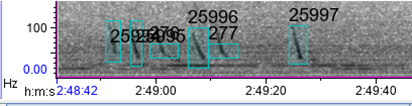
*Figure 2. Spectrogram of Pygmy blue whale D calls manually (and automatically) selected, frequency 0-150 Hz.*

Understanding research on blue whales

The most difficult part about coming into a project as an outsider is catching up. I learned how anthropogenetic (human made) noise affects blue whale communication. For example, it has been showing that Mid Frequency Active Sonar signals employed by the U.S. Navy affect blue whale D calling patterns (Melcón 2012). Furthermore, noise from seismic airguns used for oil and gas exploration has also impact blue whale calling behavior (Di Lorio, 2010). Understanding the environmental context in which the pygmy blue whales live and the anthropogenic pressures they face is essential in marine conservation. Protecting the areas in which they live is important so they can feed, reproduce and thrive effectively. What began as a slowly falling snowflake at the start of a snowstorm turned into a cascading avalanche of knowledge pouring into my mind in just two weeks.

*Figure 3. The white stars show the hydrophone locations (n = 5). A bathymetric scale of the depth is also given.*

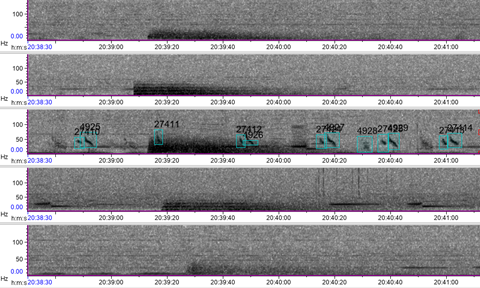
The research question I set out to tackle in my internship was: do blue whales change their calling behavior in response to natural noise events from earthquake activity? To do this, I used acoustic recordings from five hydrophones deployed in the South Taranaki Bight (Fig. 3), paired with an existing dataset of all recorded earthquakes in New Zealand (GeoNet). I identified known earthquakes in our acoustic recordings, and then examined the blue whale D calls during 4 hours before and after each earthquake event to look for any change in the number of calls, call energy, entropy, or bandwidth.

A great mentor and lab team

The days kept passing and blending into each other, as they often do with remote work. I began to feel isolated from the people I was working with and the blue whales I was studying. The zoom calls, group chats, and working alongside other remote interns kept me afloat as I adapted to a work world fully online. Nevertheless, I was happy to continue working on this project because I felt like I was slowly becoming part of the GEMM Lab. I would meet with my mentor Dawn Barlow at least once a week and we would spend time talking about the project and sorting out the difficult details of data processing. She always encouraged my curiosity to ask questions. Even if they were silly questions, she was happy to ponder them because she is a curious scientist like myself.

What we learned

Pygmy blue whales from the South Taranaki Bight region do not change their acoustic behavior in response to earthquake activity. The energy of the earthquake, magnitude, depth, and distance to the origin all had no influence on the number of blue whale D calls, the energy of their calling, the entropy, and the bandwidth. A likely reason for why the blue whales would have no acoustic response to earthquakes (magnitude < 5) is that the STB region is a seismically active region due to the nearby interface of the Australian and Pacific plates. Because of the plate tectonics, the region averages about 20,000 recorded earthquakes per year (GeoNet: Earthquake Statistics). Given that pygmy blue whales are present in the STB region year-round (Barlow et al. 2018), the blue whales may have adapted to tolerate the earthquake activity (Fig 4).

*Figure 4. Earthquake signal from MARU (1, 2, 3, 4, 5) and blue whale D calls, Frequency 0-150 Hz.*

Looking at the future

I presented my work at the end of my REU internship program, which was a difficult challenge for me because I am often intimidated by public speaking (who isn’t?). Communicating science has always been a big interest of me. I love reading news articles about new breakthroughs and being a small part of that is a huge privilege for me. Finding my own voice and having new insights to contribute to the scientific world has always been my main objective. Now I will get to deliver a poster presentation of my REU work at the Association for the Sciences of Limnology and Oceanography (ASLO) Conference in March 2022. I am both excited and nervous to take on this new adventure of meeting seasoned professionals, communicating my results, and learning about the ocean sciences. I hope to gain new inspirations for my future academic and professional work.

References:

About Earthquake Drums – GeoNet. geonet.Org. Retrieved June 23, 2021, from https://www.geonet.org.nz/about/earthquake/drums

Barlow, D. R., Torres, L. G., Hodge, K. B., Steel, D., Scott Baker, C., Chandler, T. E., Bott, N., Constantine, R., Double, M. C., Gill, P., Glasgow, D., Hamner, R. M., Lilley, C., Ogle, M., Olson, P. A., Peters, C., Stockin, K. A., Tessaglia-Hymes, C. T., & Klinck, H. (2018). Documentation of a New Zealand blue whale population based on multiple lines of evidence. Endangered Species Research, 36, 27–40. https://doi.org/10.3354/esr00891

Di Iorio, L., & Clark, C. W. (2010). Exposure to seismic survey alters blue whale acoustic communication. Biology Letters, 6(3), 334–335. https://doi.org/10.1098/rsbl.2009.0967

Lewis, L. A., Calambokidis, J., Stimpert, A. K., Fahlbusch, J., Friedlaender, A. S., McKenna, M. F., Mesnick, S. L., Oleson, E. M., Southall, B. L., Szesciorka, A. R., & Sirović, A. (2018). Context-dependent variability in blue whale acoustic behaviour. Royal Society Open Science, 5(8). https://doi.org/10.1098/rsos.180241

Melcón, M. L., Cummins, A. J., Kerosky, S. M., Roche, L. K., Wiggins, S. M., & Hildebrand, J. A. (2012). Blue whales respond to anthropogenic noise. PLoS ONE, 7(2), 1–6. https://doi.org/10.1371/journal.pone.0032681

Torres LG. 2013 Evidence for an unrecognised blue whale foraging ground in New Zealand. NZ J. Mar. Freshwater Res. 47, 235–248. (doi:10. 1080/00288330.2013.773919)

Share this:

Share this:

References

Share this:

Share this:

Share this:

Share this:

Share this:

Share this:

Share this:

Share this: