Marine heatwaves and their impact on marine mammals

By Dawn Barlow, PhD student, OSU Department of Fisheries and Wildlife, Geospatial Ecology of Marine Megafauna Lab

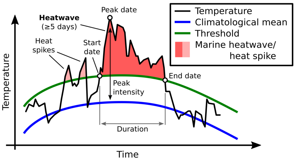
In recent years, anomalously warm ocean temperatures known as “marine heatwaves” have sparked considerable attention and concern around the world. Marine heatwaves (MHW) occur when seawater temperatures rise above a seasonal threshold (greater than the 90th percentile) for five consecutive days or longer (Hobday et al. 2016; Fig. 1). With global ocean temperatures continuing to rise, we are likely to see more frequent and more intense MHW conditions in the future. Indeed, the global prevalence of MHWs is increasing, with a 34% rise in frequency, a 17%  increase in duration, and a 54% increase in annual MHW days globally since 1925 (Oliver et al. 2018). With sustained anomalously warm water temperatures come a range of ecological, sociological, and economic consequences. These impacts include changes in water column structure, primary production, species composition, marine life distribution and health, and fisheries management including closures and quota changes (Oliver et al. 2018).

Figure 1. Illustration of how marine heatwaves are defined. Source: marineheatwaves.org

The notorious “warm blob” was an MHW event that plagued the northeast Pacific Ocean from 2014-2016. Some of the most notable consequences of this MHW were extremely high levels of domoic acid, extreme changes in the biodiversity of pelagic species, and an unprecedented delay in the opening of the Dungeness crab fishery, which is an important and lucrative fishery for the West Coast of the United States (Santora et al. 2020). The “warm blob” directly impacted the California Current ecosystem, which is typically a highly productive coastal area driven by seasonal upwelling. Yet, as a consequence of the 2014-2016 MHW, upwelling habitat was compressed and constricted to the coastal boundary, resulting in a contraction in available habitat for humpback whales and a shift in their prey (Santora et al. 2020; Fig. 2).

Figure 2. A figure from Santora et al. 2020 illustrating the compression in available upwelling habitat, defined by areas with SST<12°C (delineated by the black line), during the 2014-2016 marine heatwave in the California Current ecosystem.

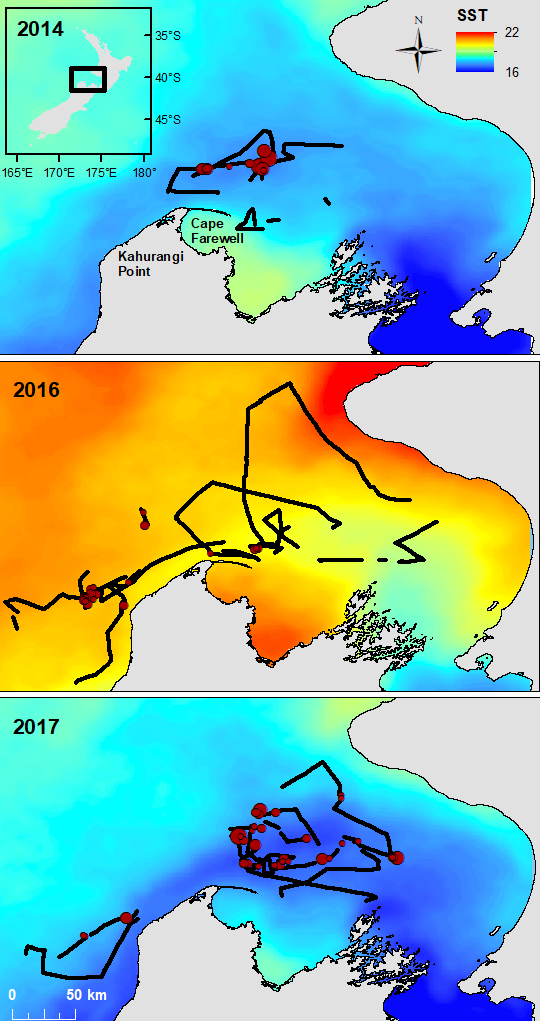
Shifting to an example from another part of the world, the austral summer of 2015-2016 coincided with a strong regional MHW in the Tasman Sea between Australia and New Zealand, which lasted for 251 days and had a maximum intensity of 2.9°C above the climatological average (Oliver et al. 2017). Subsequently, the conditions were linked to a significant shift in zooplankton species composition and abundance in Australia (Evans et al. 2020). Ocean warming, including MHWs, also appears to decrease primary production in the Tasman Sea and large portions of New Zealand’s marine ecosystem (Chiswell & Sutton 2020). In New Zealand’s South Taranaki Bight region, where we study the ecology of blue whales, we observed a shift in blue whale distribution in the MWH conditions of February 2016 relative to more typical ocean conditions in 2014 and 2017 (Fig. 3). The first chapter of my dissertation includes a detailed analysis of the impacts of the 2016 MHW on New Zealand oceanography, krill, and blue whales, documenting how the warm, stratified water column of 2016 led to consequences across multiple trophic levels, from phytoplankton, to zooplankton, to whales.

Figure 3. Maps showing monthly sea surface temperature (SST) in the South Taranaki Bight region of New Zealand during our three years of survey effort to document blue whale distribution (February 2014, 2016, and 2017). Vessel tracklines are shown in black, with blue whale sighting locations shown in dark red. Red circles are scaled by the number of blue whales observed at each sighting. The color ramp of SST values is consistent across the three maps, making the dramatically warmer ocean conditions of 2016 evident.

The response of marine mammals is tightly linked to shifts in their environment and prey (Silber et al. 2017). With MHWs and changing ocean conditions, there will likely be “winners” and “losers” among marine predators including large whales. Blue whales are highly selective krill specialists (Nickels et al. 2019), whereas other species of whales, such as humpback whales, have evolved flexible feeding tactics that allow them to switch target prey species when needed (Cade et al. 2020). In California, humpback whales have been shown to switch their primary prey from krill to fish during warm years (Fossette et al. 2017, Santora et al. 2020). By contrast, blue whales shift their distribution in response to changing krill availability during warm years (Fossette et al. 2017), however this strategy comes with increased risk and energetic cost associated with searching for prey in new areas. Furthermore, in instances when a prey resource such as krill becomes increasingly scarce for a multi-year period (Santora et al. 2020), krill specialist predators such as blue whales are at a considerable disadvantage. It is also important to acknowledge that although the humpbacks in California may at first seem to have a winning strategy for adaptation by switching their food source, this tactic may come with unforeseen consequences. Their distribution overlapped substantially with Dungeness crab fishing gear during MHW conditions in the warm blob years, resulting in record numbers of entanglements that may have population-level repercussions (Santora et al. 2020).

While this is certainly not the most light-hearted blog topic, I believe it is an important one. As warming ocean temperatures contribute to the increase in frequency, intensity, and duration of extreme conditions such as MHW events, it is paramount that we understand their impacts and take informed management actions to mitigate consequences, such as lethal entanglements as a result of compressed whale habitat. But perhaps more importantly, even as we do our best to manage consequences, it is critical that we as individuals realize the role we have to play in reducing the root cause of warming oceans, by being conscious consumers and being mindful of the impact our actions have on the climate. 

References

Cade DE, Carey N, Domenici P, Potvin J, Goldbogen JA (2020) Predator-informed looming stimulus experiments reveal how large filter feeding whales capture highly maneuverable forage fish. Proc Natl Acad Sci USA.

Chiswell SM, Sutton PJH (2020) Relationships between long-term ocean warming, marine heat waves and primary production in the New Zealand region. New Zeal J Mar Freshw Res.

Evans R, Lea MA, Hindell MA, Swadling KM (2020) Significant shifts in coastal zooplankton populations through the 2015/16 Tasman Sea marine heatwave. Estuar Coast Shelf Sci.

Fossette S, Abrahms B, Hazen EL, Bograd SJ, Zilliacus KM, Calambokidis J, Burrows JA, Goldbogen JA, Harvey JT, Marinovic B, Tershy B, Croll DA (2017) Resource partitioning facilitates coexistence in sympatric cetaceans in the California Current. Ecol Evol.

Hobday AJ, Alexander L V., Perkins SE, Smale DA, Straub SC, Oliver ECJ, Benthuysen JA, Burrows MT, Donat MG, Feng M, Holbrook NJ, Moore PJ, Scannell HA, Sen Gupta A, Wernberg T (2016) A hierarchical approach to defining marine heatwaves. Prog Oceanogr.

Nickels CF, Sala LM, Ohman MD (2019) The euphausiid prey field for blue whales around a steep bathymetric feature in the southern California current system. Limnol Oceanogr.

Oliver ECJ, Benthuysen JA, Bindoff NL, Hobday AJ, Holbrook NJ, Mundy CN, Perkins-Kirkpatrick SE (2017) The unprecedented 2015/16 Tasman Sea marine heatwave. Nat Commun.

Oliver ECJ, Donat MG, Burrows MT, Moore PJ, Smale DA, Alexander L V., Benthuysen JA, Feng M, Sen Gupta A, Hobday AJ, Holbrook NJ, Perkins-Kirkpatrick SE, Scannell HA, Straub SC, Wernberg T (2018) Longer and more frequent marine heatwaves over the past century. Nat Commun.

Santora JA, Mantua NJ, Schroeder ID, Field JC, Hazen EL, Bograd SJ, Sydeman WJ, Wells BK, Calambokidis J, Saez L, Lawson D, Forney KA (2020) Habitat compression and ecosystem shifts as potential links between marine heatwave and record whale entanglements. Nat Commun.

Silber GK, Lettrich MD, Thomas PO, Baker JD, Baumgartner M, Becker EA, Boveng P, Dick DM, Fiechter J, Forcada J, Forney KA, Griffis RB, Hare JA, Hobday AJ, Howell D, Laidre KL, Mantua N, Quakenbush L, Santora JA, Stafford KM, Spencer P, Stock C, Sydeman W, Van Houtan K, Waples RS (2017) Projecting marine mammal distribution in a changing climate. Front Mar Sci.

Eyes from Space: Using Remote Sensing as a Tool to Study the Ecology of Blue Whales

By Christina Garvey, University of Maryland, GEMM Lab REU Intern

It is July 8th and it is my 4th week here in Hatfield as an REU intern for Dr. Leigh Torres. My name is Christina Garvey and this summer I am studying the spatial ecology of blue whales in the South Taranaki Bight, New Zealand. Coming from the east coast, Oregon has given me an experience of a lifetime – the rugged shorelines continue to take my breath away and watching sea lions in Yaquina Bay never gets old. However, working on my first research project has by far been the greatest opportunity and I have learned so much in so little time. When Dr. Torres asked me to contribute to this blog I was unsure of how I would write about my work thus far but I am excited to have the opportunity to share the knowledge I have gained with whoever reads this blog post.

The research project that I will be conducting this summer will use remotely sensed environmental data (information collected from satellites) to predict blue whale distribution in the South Taranaki Bight (STB), New Zealand. Those that have read previous blogs about this research may remember that the STB study area is created by a large indentation or “bight” on the southern end of the Northern Island. Based on multiple lines of evidence, Dr. Leigh Torres hypothesized the presence of an unrecognized blue whale foraging ground in the STB (Torres 2013). Dr. Torres and her team have since proved that blue whales frequent this region year-round; however, the STB is also very industrial making this space-use overlap a conservation concern (Barlow et al. 2018). The increasing presence of marine industrial activity in the STB is expected to put more pressure on blue whales in this region, whom are already vulnerable from the effects of past commercial whaling (Barlow et al. 2018) If you want to read more about blue whales in the STB check out previous blog posts that talk all about it!

Figure 1. A blue whale surfaces in front of a floating production storage and offloading vessel servicing the oil rigs in the South Taranaki Bight. Photo by D. Barlow.

Figure 2. South Taranaki Bight, New Zealand, our study site outlined by the red box. Kahurangi Point (black star) is the site of wind-driven upwelling system.

The possibility of the STB as an important foraging ground for a resident population of blue whales poses management concerns as New Zealand will have to balance industrial growth with the protection and conservation of a critically endangered species. As a result of strong public support, there are political plans to implement a marine protected area (MPA) in the STB for the blue whales. The purpose of our research is to provide scientific knowledge and recommendations that will assist the New Zealand government in the creation of an effective MPA.

In order to create an MPA that would help conserve the blue whale population in the STB, we need to gather a deeper understanding of the relationship between blue whales and this marine environment. One way to gain knowledge of the oceanographic and ecological processes of the ocean is through remote sensing by satellites, which provides accessible and easy to use environmental data. In our study we propose remote sensing as a tool that can be used by managers for the design of MPAs (through spatial and temporal boundaries). Satellite imagery can provide information on sea surface temperature (SST), SST anomaly, as well as net primary productivity (NPP) – which are all measurements that can help describe oceanographic upwelling, a phenomena that is believed to be correlated to the presence of blue whales in the STB region.

Figure 3. The stars of the show: blue whales. A photograph captured from the small boat of one animal fluking up to dive down as another whale surfaces close by. (Photo credit: L. Torres)

Past studies in the STB showed evidence of a large upwelling event that occurs off the coast of Kahurangi Point (Fig. 2), on the northwest tip of the South Island (Shirtcliffe et al. 1990). In order to study the relationship of this upwelling to the distribution of blue whales, I plan to extract remotely sensed data (SST, SST anomaly, & NPP) off the coast of Kahurangi and compare it to data gathered from a centrally located site within the STB, which is close to oil rigs and so is of management interest. I will first study how decreases in sea surface temperature at the site of upwelling (Kahurangi) are related to changes in sea surface temperature at this central site in the STB, while accounting for any time differences between each occurrence. I expect that this relationship will be influenced by the wind patterns, and that there will be changes based on the season. I also predict that drops in temperature will be strongly related to increases in primary productivity, since upwelling brings nutrients important for photosynthesis up to the surface. These dips in SST are also expected to be correlated to blue whale occurrence within the bight, since blue whale prey (krill) eat the phytoplankton produced by the productivity.

Figure 4. A blue whale lunges on an aggregation of krill. UAS piloted by Todd Chandler.

To test the relationships I determine between remotely sensed data at different locations in the STB, I plan to use blue whale observations from marine mammal observers during a seismic survey conducted in 2013, as well as sightings recorded from the 2014, 2016, and 2017 field studies led by Dr. Leigh Torres. By studying the statistical relationships between all of these variables I hope to prove that remote sensing can be used as a tool to study and understand blue whale distribution.

I am very excited about this research, especially because the end goal of creating an MPA really gives me purpose. I feel very lucky to be part of a project that could make a positive impact on the world, if only in just a little corner of New Zealand. In the mean time I’ll be here in Hatfield doing the best I can to help make that happen.

References: 

Barlow DR, Torres LG, Hodge KB, Steel D, Baker CS, Chandler TE, Bott N, Constantine R, Double MC, Gill P, Glasgow D, Hamner RM, Lilley C, Ogle M, Olson PA, Peters C, Stockin KA, Tessaglia-hymes CT, Klinck H (2018) Documentation of a New Zealand blue whale population based on multiple lines of evidence. Endanger Species Res 36:27–40.

Shirtcliffe TGL, Moore MI, Cole AG, Viner AB, Baldwin R, Chapman B (1990) Dynamics of the Cape Farewell upwelling plume, New Zealand. New Zeal J Mar Freshw Res 24:555–568.

Torres LG (2013) Evidence for an unrecognised blue whale foraging ground in New Zealand. New Zeal J Mar Freshw Res 47:235–248.

Species distribution modeling: Part statistics, part philosophy, and there is no “right answer”

By Dawn Barlow, PhD student, OSU Department of Fisheries and Wildlife, Geospatial Ecology of Marine Megafauna Lab

Just like that, I have wrapped up year 1 of my PhD in Wildlife Science. For my PhD, I am investigating the ecology and distribution of blue whales in New Zealand across multiple spatial and temporal scales. In a region where blue whales overlap with industrial activity, there is considerable interest from managers to be able to reliably forecast when and where blue whales are most likely to be in the area. In a series of five chapters and utilizing multiple different data sources (dedicated boat surveys, oceanographic data, acoustic recordings, remotely sensed environmental data, opportunistic blue whale sightings information), I will attempt to describe, quantify, and predict where blue whales are found in relation to their environment. Each chapter will evaluate the distribution of blue whales relative to the environment at different scales in space (ranging from 4 km to 25 km resolution) and time (ranging from daily to seasonal resolution). One overarching method I am using throughout my PhD is species distribution modeling. Having just completed my research review with my doctoral committee last week, I’ll share this aspect of my research proposal that I’ve particularly enjoyed reading, writing, and thinking about.

A pair of blue whales surfacing in the South Taranaki Bight region of New Zealand. Drone piloted by Todd Chandler during the 2017 field season.

Species distribution models (SDMs), which are sometimes referred to as habitat models or ecological niche models, are mathematical algorithms that combine observations of a species with environmental conditions at their observed locations, to gain ecological insight and predict spatial distributions of the species (Elith and Leathwick, 2009; Redfern et al., 2006). Any model is just one description of what is occurring in the natural world. Just as there are many ways to describe something with words and many languages to do so, there are many options for modeling frameworks and approaches, with stark and nuanced differences. My labmate and friend Solene Derville has equated the number of choices one has for SDMs to the cracker section in an American grocery store. When navigating all of these choices and considerations, it is important to remember that no model will ever be completely correct—it is our best attempt at describing a complex natural system—and as an analyst we need to do the best that we can with the data available to address the ecological questions at hand. As it turns out, the dividing line between quantitative analysis and philosophy is thin at times. What may seem at first like a purely objective, statistical endeavor requires careful consideration and fundamental decision-making on the part of the analyst.

Ecosystems are multifaceted, complex, and hierarchical. They are comprised of multiple physical and biological components, which operate at multiple scales across space and time. As Dr. Simon Levin stated in at 1989 MacArthur Award lecture on the topic of scale in ecology:

“A good model does not attempt to reproduce every detail of the biological system; the system itself suffices for that purpose as the most detailed model of itself. Rather, the objective of a model should be to ask how much detail can be ignored without producing results that contradict specific sets of observations, on particular scales of interest” (Levin, 1992).

The question of scale is central to ecology. As many biology students learn in their first introductory classes, parsimony is “The principle that the most acceptable explanation of an occurrence, phenomenon, or event is the simplest, involving the fewest entities, assumptions, or changes” (Oxford Dictionary). In other words, the best explanation is the simplest one. One challenge in ecological modeling, including SDMs, is to select spatial and temporal scales as coarse as possible for the most parsimonious—the most straightforward—model, while still being fine enough to capture relevant patterns. Another critical consideration is the scale of the question you are interested in answering. The scale of the analysis must match the scale at which you want to make inferences about the ecology of a species.

Similarly, the issue of complexity is central to distribution modeling. Overly simple models may not be able to adequately describe the relationship between species occurrence and the environment. In contrast, highly complex models may have very high explanatory power, but risk ascribing an ecological pattern to noise in the data (Merow et al., 2014), in other words, finding patterns that aren’t real. Furthermore, highly complex models tend to have poorer predictive capacity than simpler models (Merow et al., 2014). There is a trade-off between descriptive and predictive power in SDMs (Derville et al., 2018). Therefore, a key component in the SDM process is establishing the end goal of the model with respect to the region of interest, scale, explanatory power, predictive capacity, and in many cases management need.

Finally, any model is ultimately limited by the data available and the scale at which it was collected (Elith and Leathwick, 2009; Guillera-Arroita et al., 2015; Redfern et al., 2006). Prior knowledge of what environmental features are important to the species of interest is often limited at the time of the data collection effort, and data collection is constrained by when it is logistically feasible to sample. For example, we collect detailed oceanographic data during the summer months when it is practical to get out on the water, satellite imagery of sea surface temperature might be unavailable during times of cloud cover, and people are more likely to report blue whale sightings in areas where there is more human activity. Therefore, useful SDMs that address both ecological and management needs typically balance the scale of analysis and model complexity with the limitations of the data.

Managers and politicians within the New Zealand government are interested in a tool to predict when and where blue whales are most likely to be, based on sound ecological analysis. This is one of the end-goals of my PhD, but in the meantime, I am grappling with the appropriate scales of analysis, and attempting to balance questions of model complexity, explanatory power, and predictive capacity. There is no single, correct answer, and so my process is in part quantitative analysis, part philosophy, and all with the goal of increased ecological understanding and conservation of a species.

A blue whale breaks the surface. As I grapple with questions of model complexity and scale of analysis, I sometimes need a reminder that behind each data point is a blue whale, and what a privilege it is to study them. Photo by Leigh Torres.

References:

Derville, S., Torres, L. G., Iovan, C., and Garrigue, C. (2018). Finding the right fit: Comparative cetacean distribution models using multiple data sources and statistical approaches. Divers. Distrib. 24, 1657–1673. doi:10.1111/ddi.12782.

Elith, J., and Leathwick, J. R. (2009). Species Distribution Models: Ecological Explanation and Prediction Across Space and Time. Annu. Rev. Ecol. Evol. Syst. 40, 677–697. doi:10.1146/annurev.ecolsys.110308.120159.

Guillera-Arroita, G., Lahoz-Monfort, J. J., Elith, J., Gordon, A., Kujala, H., Lentini, P. E., et al. (2015). Is my species distribution model fit for purpose? Matching data and models to applications. Glob. Ecol. Biogeogr. 24, 276–292. doi:10.1111/geb.12268.

Levin, S. A. (1992). The problem of pattern and scale. Ecology 73, 1943–1967.

Merow, C., Smith, M. J., Edwards, T. C., Guisan, A., Mcmahon, S. M., Normand, S., et al. (2014). What do we gain from simplicity versus complexity in species distribution models? Ecography (Cop.). 37, 1267–1281. doi:10.1111/ecog.00845.

Redfern, J. V., Ferguson, M. C., Becker, E. A., Hyrenbach, K. D., Good, C., Barlow, J., et al. (2006). Techniques for cetacean-habitat modeling. Mar. Ecol. Prog. Ser. 310, 271–295. doi:10.3354/meps310271.

The “demon whale-biter”, and why I am learning about an elusive little shark

By Dawn Barlow, PhD student, OSU Department of Fisheries and Wildlife, Geospatial Ecology of Marine Megafauna Lab

There is an ancient Samoan legend that upon entry into a certain bay in Samoa, tuna would sacrifice pieces of their flesh to the community chief1. This was the explanation given for fish with circular shaped wounds where a plug of flesh had been removed. Similar round wounds are also observed on swordfish2, sharks3, and marine mammals including whales4,5, dolphins6, porpoises7, and pinnipeds8,9. In 1971, Everet C. Jones posited that the probable cause of these crater wounds was a small shark only 42-56 cm in length, Isistius brasiliensis1. The species was nicknamed “demon whale-biter” by Stewart Springer, who subsequently popularized the common name for the species, cookie cutter shark.

Figure 1. A yellowfin tuna with a circular bite, characteristic of a cookie cutter shark (Isistius brasiliensis). Photo: John Soward.

I am currently preparing a manuscript on blue whale skin condition. While this is only tangentially related to my doctoral research, it is an exciting side project that has encouraged me to stretch my comfort zone as an ecologist. This analysis of skin condition is part of a broader health assessment of blue whales in New Zealand, where we will be linking skin lesion severity with stress and reproductive hormone levels as well as body condition. Before I continue, I owe a major shout-out to Acacia Pepper, a senior undergraduate student at Oregon State University who has been working with me for nearly the past year through the Fisheries and Wildlife mentorship program. Acacia’s rigor in researching methodologies led us to develop a comprehensive protocol that can be applied widely to any cetacean photo-identification catalog. This method allows us to quantify prevalence and severity of different marking types in a standardized manner. Her passion for marine mammal science and interest in the subject matter is enough to excite this ecologist into fascination with wound morphology and blister concavity. Next thing you know, we are preparing a paper for publication together with P.I. Dr. Leigh Torres on a comprehensive skin condition assessment of blue whales that includes multiple markings and lesion types, but for the purpose of this blog post, I will share just a “bite-sized” piece of the story.

Figure 2. Jaws of a cookie cutter shark. Photo: George Burgess.

Back to the demon whale-biter. What do we know about cookie cutter sharks? Not a whole lot, it turns out. They are elusive, and are thought to live in deep (>1,000 m), offshore waters. They are considered to be both an ectoparasite and an ambush predator. Their distribution is tropical and sub-tropical. Much of what we know and assume about their distribution comes from the bite wounds they leave on their prey2.

In New Zealand where we study a unique population of blue whales10, the southernmost record of cookie cutter sharks is ~ 39⁰S11. We found that in our dataset of 148 photo-identified blue whales, 96% were affected by cookie cutter shark bites. Furthermore, 38% were categorized as having “severe” cookie cutter bite wounds or scars. The latitude of our blue whale sightings ranges from 29-48⁰S and blue whales are highly mobile, so any of the whales in our dataset could theoretically swim in and out of the known range of cookie cutter sharks. In our skin condition assessment, we also categorized cookie cutter bite “freshness” and phase of healing as follows:

We wanted to know if the freshness of cookie cutter shark bites was related in to the latitude at which the whales were photographed. Of the whales photographed north of 39⁰S (n=46), 76% had phase 1 or 2 cookie cutter shark bites present. In contrast, 57.1% of whales photographed south of 39⁰S (n=133) had phase 1 or 2 cookie cutter shark bites. It therefore appears that in New Zealand, the freshness of cookie cutter shark bites on blue whales is related to the latitude at which the whales were sighted, with fresher bites being more common at more northerly latitudes.

Figure 3. A whale with fresh cookie cutter shark bites, photographed in the Bay of Islands, latitude 35.164⁰S. Photo courtesy of Dr. Catherine Peters.

Figure 4. A whale with mostly healed cookie cutter shark bites, photographed off of Kaikoura, latitude 42.464⁰S. Photo courtesy of Jody Weir.

In the midst of a PhD on distribution modeling and habitat use of blue whales, I find myself reading about Samoan legends of tuna with missing flesh and descriptions of strange circular lesions from whaling records, and writing a paper about blue whale skin condition. Exciting “side projects” like this one emerge from rich datasets and good collaboration.

References

  1. Jones, E. C. Isistius brasiliensis, a squaloid shark, the probable cause of crater wounds on fishes and cetaceans. Fish. Bull. 69, 791–798 (1971).
  2. Papastamatiou, Y. P., Wetherbee, B. M., O’Sullivan, J., Goodmanlowe, G. D. & Lowe, C. G. Foraging ecology of Cookiecutter Sharks (Isistius brasiliensis) on pelagic fishes in Hawaii, inferred from prey bite wounds. Environ. Biol. Fishes 88, 361–368 (2010).
  3. Hoyos-Padilla, M., Papastamatiou, Y. P., O’Sullivan, J. & Lowe, C. G. Observation of an Attack by a Cookiecutter Shark ( Isistius brasiliensis ) on a White Shark ( Carcharodon carcharias ) . Pacific Sci. 67, 129–134 (2013).
  4. Mackintosh, N. A. & Wheeler, J. F. G. Southern blue and fin whales. Discov. Reports 1, 257–540 (1929).
  5. Best, P. B. & Photopoulou, T. Identifying the ‘demon whale-biter’: Patterns of scarring on large whales attributed to a cookie-cutter shark Isistius sp. PLoS One 11, (2016).
  6. Heithaus, M. R. Predator-prey and competitive interactions between sharks (order Selachii) and dolphins (suborder Odontoceti): A review. J. Zool. 253, 53–68 (2001).
  7. Van Utrecht, W. L. Wounds And Scars In The Skin Of The Common Porpoise, Phocaena Phocaena (L.). Mammalia 23, 100–122 (1959).
  8. Gallo‐Reynoso, J. ‐P & Figueroa‐Carranza, A. ‐L. A COOKIECUTTER SHARK WOUND ON A GUADALUPE FUR SEAL MALE. Mar. Mammal Sci. 8, 428–430 (1992).
  9. Le Boeuf, B. J., McCosker, J. E. & Hewitt, J. Crater wounds on northern elephant seals: the cookiecutter shark strikes again. Fish. Bull. 85, 387–392 (1987).
  10. Barlow, D. R. et al. Documentation of a New Zealand blue whale population based on multiple lines of evidence. Endanger. Species Res. 36, 27–40 (2018).
  11. Dwyer, S. L. & Visser, I. N. Cookie cutter shark (Isistius sp.) bites on cetaceans, with particular reference to killer whales (Orca) (Orcinus orca). Aquat. Mamm. 37, 111–138 (2011).

More data, more questions, more projects: There’s always more to learn

By Dawn Barlow, PhD student, OSU Department of Fisheries and Wildlife, Geospatial Ecology of Marine Megafauna Lab 

As you may have read in previous blog posts, my research focuses on the ecology of blue whales in New Zealand. Through my MS research and years of work by a dedicated team, we were able to document and describe a population of around 700 blue whales that are unique to New Zealand, present year-round, and genetically distinct from all other known populations [1]. While this is a very exciting discovery, documenting this population has also unlocked a myriad of further questions about these whales. Can we predict when and where the whales are most likely to be? How does their distribution change seasonally? How often do they overlap with anthropogenic activity? My PhD research will aim to answer these questions through models of blue whale distribution patterns relative to their environment at multiple spatial and temporal scales.

Because time at sea for vessel-based surveys is cost-limited and difficult to come by, it is in any scientist’s best interest to collect as many concurrent streams of data as possible while in the field. When Dr. Leigh Torres designed our blue whale surveys that were conducted in 2014, 2016, and 2017, she really did a miraculous job of maximizing time on the water. With more data, more questions can be asked. These complimentary datasets have led to the pursuit of many “side projects”. I am lucky enough to work on these questions in parallel with what will form the bulk of my PhD, and collaborate with a number of people in the process. In this blog post, I’ll give you some short teasers of these “side projects”!

Surface lunge feeding as a foraging strategy for New Zealand blue whales

Most of what we know about blue whale foraging behavior comes from studies conducted off the coast of Southern California[2,3] using suction cup accelerometer tags. While these studies in the California Current ecosystem have led to insights and breakthroughs in our understanding of these elusive marine predators and their prey, they have also led us to adopt the paradigm that krill patches are denser at depth, and blue whales are most likely to target these deep prey patches when they feed. We have combined our prey data with blue whale behavioral data observed via a drone to investigate blue whale foraging in New Zealand, with a particular emphasis on surface feeding as a strategy. In our recent analyses, we are finding that in New Zealand, lunge feeding at the surface may be more than just “snacking”. Rather, it may be an energetically efficient strategy that blue whales have evolved in the region with unique implications for conservation.

Figure 1. A blue whale lunges on an aggregation of krill. UAS piloted by Todd Chandler.

Combining multiple data streams for a comprehensive health assessment

In the field, we collected photographs, blubber biopsy samples, fecal samples, and conducted unmanned aerial system (UAS, a.k.a. “drone”) flights over blue whales. The blubber and fecal samples can be analyzed for stress and reproductive hormone levels; UAS imagery allows us to quantify a whale’s body condition[4]; and photographs can be used to evaluate skin condition for abnormalities. By pulling together these multiple data streams, this project aims to establish a baseline understanding of the variability in stress and reproductive hormone levels, body condition, and skin condition for the population. Because our study period spans multiple years, we also have the ability to look at temporal patterns and individual changes over time. From our preliminary results, we have evidence for multiple pregnant females from elevated pregnancy and stress hormones, as well as apparent pregnancy from the body condition analysis. Additionally, a large proportion of the population appear to be affected by blistering and cookie cutter shark bites.

Figure 2. An example aerial drone image of a blue whale that will be used to asses body condition, i.e. how healthy or malnourished the whale is. (Drone piloted by Todd Chandler).

Figure 3. Images of blue whale skin condition, affected by A) blistering and B) cookie cutter shark bites.

Comparing body shape and morphology between species

The GEMM Lab uses UAS to quantitatively study behavior[5] and health of large whales. From various projects in different parts of the world we have now assimilated UAS data on blue, gray, and humpback whales. We will measure these images to investigate differences in body shape and morphology among these species. We plan to explore how form follows function across baleen whales, based on their different  life histories, foraging strategies, and ecological roles.

Figure 4 . Aerial images of A) a blue whale in New Zealand’s South Taranaki Bight, B) a gray whale off the coast of Oregon, and C) a humpback whale off the coast of Washington. Drone piloted by Todd Chandler (A and B) and Jason Miranda (C). 

So it goes—my dissertation will contain a series of chapters that build on one another to explore blue whale distribution patterns at increasing scales, as well as a growing number of appendices for these “side projects”. Explorations and collaborations like I’ve described here allow me to broaden my perspectives and diversify my analytical skills, as well as work with many excellent teams of scientists. The more data we collect, the more questions we are able to ask. The more questions we ask, the more we seem to uncover that is yet to be understood. So stay tuned for some exciting forthcoming results from all of these analyses, as well as plenty of new questions, waiting to be posed.

References

  1. Barlow DR et al. 2018 Documentation of a New Zealand blue whale population based on multiple lines of evidence. Endanger. Species Res. 36, 27–40. (doi:https://doi.org/10.3354/esr00891)
  2. Hazen EL, Friedlaender AS, Goldbogen JA. 2015 Blue whales (Balaenoptera musculus) optimize foraging efficiency by balancing oxygen use and energy gain as a function of prey density. Sci. Adv. 1, e1500469–e1500469. (doi:10.1126/sciadv.1500469)
  3. Goldbogen JA, Calambokidis J, Oleson E, Potvin J, Pyenson ND, Schorr G, Shadwick RE. 2011 Mechanics, hydrodynamics and energetics of blue whale lunge feeding: efficiency dependence on krill density. J. Exp. Biol. 214, 131–146. (doi:10.1242/jeb.048157)
  4. Burnett JD, Lemos L, Barlow DR, Wing MG, Chandler TE, Torres LG. 2018 Estimating morphometric attributes on baleen whales using small UAS photogrammetry: A case study with blue and gray whales. Mar. Mammal Sci. (doi:10.1111/mms.12527)
  5. Torres LG, Nieukirk SL, Lemos L, Chandler TE. 2018 Drone Up! Quantifying Whale Behavior From a New Perspective Improves Observational Capacity. Front. Mar. Sci. 5. (doi:10.3389/fmars.2018.00319)

More than just whales: The importance of studying an ecosystem


By Dawn Barlow, PhD student, OSU Department of Fisheries and Wildlife, Geospatial Ecology of Marine Megafauna Lab

I have the privilege of studying the largest animals on the planet: blue whales (Balaenoptera musculus). However, in order to understand the ecology, distribution, and habitat use patterns of these ocean giants, I have dedicated the past several months to studying something much smaller: krill (Nyctiphanes australis). New Zealand’s South Taranaki Bight region (“STB”, Figure 1) is an important foraging ground for a unique population of blue whales [1,2]. A wind-driven upwelling system off of Kahurangi Point (the “X” in Figure 1) generates productivity in the region [3], leading to an abundance of krill [4], the desired blue whale prey [5].

Our blue whale research team collected a multitude of datastreams in three different years, including hydroacoustic data to map krill distribution throughout our study region. The summers of 2014 and 2017 were characterized by what could be considered “typical” conditions: A plume of cold, upwelled water curving its way around Cape Farewell (marked with the star in Figure 1) and entering the South Taranaki Bight, spurring a cascade of productivity in the region. The 2016 season, however, was different. The surface water temperatures were hot, and the whales were not where we expected to find them.

Figure 2. Sea surface temperature maps of the South Taranaki Bight region in each of our three study years. The white circles indicate where most blue whale sightings were made in each year. Note the very warm temperatures in 2016, and more westerly location of blue whale sightings.

What happened to the blue whales’ food source under these different conditions in 2016? Before I share some preliminary findings from my recent analyses, it is important to note that there are many possible ways to measure krill availability. For example, the number of krill aggregations, as well as how deep, thick, and dense those aggregations are in an area will all factor into how “desirable” krill patches are to a blue whale. While there may not be “more” or “less” krill from one year to the next, it may be more or less accessible to a blue whale due to energetic costs of capturing it. Here is a taste of what I’ve found so far:

In 2016, when surface waters were warm, the krill aggregations were significantly deeper than in the “typical” years (ANOVA, F=7.94, p <0.001):

Figute 3. Boxplots comparing the median krill aggregation depth in each of our three survey years.

The number of aggregations was not significantly different between years, but as you can see in the plot below (Figure 4) the krill were distributed differently in space:

Figure 4. Map of the South Taranaki Bight region with the number of aggregations per 4 km^2, standardized by vessel survey effort. The darker colors represent areas with a higher density of krill aggregations. 

While the bulk of the krill aggregations were located north of Cape Farewell under typical conditions (2014 and 2017), in the warm year (2016) the krill were not in this area. Rather, the area with the most aggregations was offshore, in the western portion of our study region. Now, take a look at the same figure, overlaid with our blue whale sighting locations:

Figure 5. Map of standardized number of krill aggregations, overlaid with blue whale sighting locations in red stars.

Where did we find the whales? In each year, most whale encounters were in the locations where the most krill aggregations were found! Not only that, but in 2016 the whales responded to the difference in krill distribution by shifting their distribution patterns so that they were virtually absent north of Cape Farewell, where most sightings were made in the typical years.

The above figures demonstrate the importance of studying an ecosystem. We could puzzle and speculate over why the blue whales were further west in the warm year, but the story that is emerging in the krill data may be a key link in our understanding of how the ecosystem responds to warm conditions. While the focus of my dissertation research is blue whales, they do not live in isolation. It is through understanding the ecosystem-scale story that we can better understand blue whale ecology in the STB. As I continue modeling the relationships between oceanography, krill, and blue whales in warm and typical years, we are beginning to scratch the surface of how blue whales may be responding to their environment.

  1. Torres LG. 2013 Evidence for an unrecognised blue whale foraging ground in New Zealand. New Zeal. J. Mar. Freshw. Res. 47, 235–248. (doi:10.1080/00288330.2013.773919)
  2. Barlow DR et al. 2018 Documentation of a New Zealand blue whale population based on multiple lines of evidence. Endanger. Species Res. 36, 27–40. (doi:https://doi.org/10.3354/esr00891)
  3. Shirtcliffe TGL, Moore MI, Cole AG, Viner AB, Baldwin R, Chapman B. 1990 Dynamics of the Cape Farewell upwelling plume, New Zealand. New Zeal. J. Mar. Freshw. Res. 24, 555–568. (doi:10.1080/00288330.1990.9516446)
  4. Bradford-Grieve JM, Murdoch RC, Chapman BE. 1993 Composition of macrozooplankton assemblages associated with the formation and decay of pulses within an upwelling plume in greater cook strait, New Zealand. New Zeal. J. Mar. Freshw. Res. 27, 1–22. (doi:10.1080/00288330.1993.9516541)
  5. Gill P. 2002 A blue whale (Balaenoptera musculus) feeding ground in a southern Australian coastal upwelling zone. J. Cetacean Res. Manag. 4, 179–184.

GEMM Lab 2018: A Year in the Life

By Dawn Barlow, PhD student, Department of Fisheries & Wildlife, Geospatial Ecology of Marine Megafauna Lab

As 2018 draws to a close, it is gratifying to step back and appreciate the accomplishments of the past year. For all members of the GEMM Lab, 2018 has certainly been one for the books! Here are some of our highlights for your holiday enjoyment.

We conducted fieldwork to collect new data in multiple seasons, multiple hemispheres, and across oceans. For the first time, GEMM Lab members joined the Northern California Current Ecosystem cruises aboard NOAA ship Bell M. Shimada as marine mammal observers—Florence in February, Alexa in May, and me in September.

Summertime in the Pacific Northwest brings the gray whales to the Oregon Coast. The drone-flying, poop-scooping, plankton-trapping team of Leigh, Todd, Leila, Joe, and Sharon took to the water for the third year to investigate the health of this gray whale population. It was a successful field season, ending with 72 fecal samples collected! Visiting students joined our experienced members to shadow the gray whale fieldwork—Julia Stepanuk and Alejandro Fernandez Ajo came from across the country to hop on board with us for a bit. Friendship and collaboration were built quickly in a little boat chasing after whale poop, bonding over peanut butter and jelly sandwiches.

Another GEMM Lab team tracked the gray whales from the cliff in Port Orford. Lisa Hildebrand joined us as the GEMM Lab’s newest graduate student, and immediately led a team of interns on Oregon’s southern coast to track gray whale movements and sample their prey from a trusty research kayak.

The summer 2018 gray whale foraging ecology team, affectionately known as “team whale storm”, at the Port Orford Field Station.

Rachael observed seabirds from Yaquina Head in May and June, where the colony of common murres had the highest reproductive success in 10 years! Then she left the summertime in July to travel to the other end of the world, braving winter in the remote South Atlantic to study South American fur seals in the Falkland Islands.

Dr. Rachael Orben and Dr. Alistair Bayliss looking out towards the fur seals. Photo: Kayleigh Jones

In New Caledonia, Solene and a research team ventured to Antigonia Seamount and Orne Bank to study the use of these offshore areas by breeding humpback whales. They collected numerous biopsy samples and successfully deployed satellite tags. Solene was also selected to receive the Louis Herman research scholarship to continue studying humpback whale movement and diving behavior around seamounts.

Sorting biopsy samples during a successful expedition to study humpback whales around remote seamounts in the South Pacific.

Beyond fieldwork, our members have been busily disseminating our findings. In July, Leigh and I traveled to Wellington to present our latest findings on New Zealand blue whales to scientists, managers, politicians, industry representatives, and advocacy groups. Because of our documentation of a unique New Zealand blue whale population, which was published earlier this year, the New Zealand government has proposed to create a Marine Mammal Sanctuary for the protection of blue whales. This is quite a feat, considering blue whales were classified as only “migrant” in New Zealand waters prior to our work. Fueled by flat whites in wintery Wellington, we navigated government buildings, discussing blue whale distribution patterns, overlap with the oil and gas industry, what we now know based on our latest analyses, and what we consider to be the most pressing gaps in our knowledge.

Dr. Leigh Torres and Dawn Barlow in front of Parliament in Wellington, New Zealand following the presentation of their recent findings.

Alexa spent the summer and fall in San Diego, where she collaborated with researchers at NOAA Southwest Fisheries Science Center on her study of about the health of bottlenose dolphins off the California coast. Her time down south has been productive and we look forward to having her back in Oregon with us to round out the second year of her PhD program.

In the fall, Dom and Leigh participated in the first ever Oregon Sea Otter Status of Knowledge Symposium. With growing interest in a potential sea otter reintroduction, the symposium brought together a range of experts – including scientists, managers, and tribes – to discuss what we currently know about sea otters in other regions and how this knowledge could be applied to an Oregon reintroduction effort. Dom was one of many speakers at this event, and gave a well-received talk on Oregon’s previous sea otter reintroduction attempt and brief discussion on his thesis research. Over the next year, Dom not only plans to finish his thesis, but also to join an interdisciplinary research team to further investigate other social, genetic, and ecological implications of a potential sea otter reintroduction.

Sea otter mom and pup. Source: Hakai Magazine.

2018-19 OSU NRT Cohort. Source: Oregon State University.

Several GEMM Lab members reached academic milestones this year. Rachael was promoted to Assistant Professor in the spring! She now leads the Seabird Oceanography Lab, and remains involved in multiple projects studying seabirds and pinnipeds all over the world. Leila passed her PhD qualifying exams and advanced to candidacy in the spring, a major accomplishment toward completing her doctoral degree. I successfully defended my MS degree in June, and my photo was added to our wall gallery of GEMM Lab graduates. I won’t be leaving the GEMM Lab anytime soon, however, as I will be continuing my research on New Zealand blue whales as a PhD student. The GEMM Lab welcomed a new MS student in the summer—Lisa Hildebrand will be studying gray whale foraging ecology on the Oregon Coast. Welcome, Lisa! In early December, Solene successfully defended her PhD, officially becoming Dr. Derville. Congratulations to all on these milestones, and congratulations to Leigh for continuing to grow such a successful lab and guiding us all toward these accomplishments.

Dawn Barlow answers questions during her M.Sc. defense seminar.

Dr. Solene Derville and co-supervisors Dr. Claire Garrigue and Dr. Leigh Torres after a successful PhD Defense!

Perhaps you’re looking to do some reading over the holidays? The GEMM Lab has been publishing up a storm this year! The bulletin board outside our lab is overflowing with new papers. Summarizing our work and sharing our findings with the scientific community is a critical piece of what we do. The 21 new publications this year in 14 scientific journals include contributions from Leigh (13), Rachael (3), Solene (3), Leila (6), Florence (1), Amanda (1), Erin (1), Courtney (1), Theresa (1), and myself (3). Scroll down to the end of this post to see the complete list!

If you are reading this, thank you for your support of our lab, our members, and our work. Our successes come not only from our individual determination, but more importantly from our support of one another and the support of our communities. We look forward to what’s ahead in 2019. Happy holidays from the GEMM Lab!

The whole GEMM Lab (lab dogs included) gathered for an evening playing “Evolution” at Leigh’s house.

Barlow, D. R., Torres, L. G., Hodge, K. B., Steel, D., Baker, C. S., Chandler, T. E., Bott, N., Constantine, R., Double, M. C., Gill, P., Glasgow, D., Hamner, R. M., Lilley, C., Ogle, M., Olson, P. A., Peters, C., Stockin, K. A., Tessaglia-Hymes, C. T., & Klinck, H. (2018). Documentation of a New Zealand blue whale population based on multiple lines of evidence. Endangered Species Research36, 27-40.

Barlow, D. R., Fournet, M., & Sharpe, F. (2018). Incorporating tides into the acoustic ecology of humpback whales. Marine Mammal Science.

Baylis, A. M., Tierney, M., Orben, R. A., Staniland, I. J., & Brickle, P. (2018). Geographic variation in the foraging behaviour of South American fur seals. Marine Ecology Progress Series596, 233-245.

Bishop, A., Brown, C., Rehberg, M., Torres, L., & Horning, M. (2018). Juvenile Steller sea lion (Eumetopias jubatus) utilization distributions in the Gulf of Alaska. Movement ecology6(1), 6.

Burnett, J. D., Lemos, L., Barlow, D., Wing, M. G., Chandler, T., & Torres, L. G. (2018). Estimating morphometric attributes of baleen whales with photogrammetry from small UASs: A case study with blue and gray whales. Marine Mammal Science.

Cardoso, M. D., Lemos, L. S., Roges, E. M., de Moura, J. F., Tavares, D. C., Matias, C. A. R., … & Siciliano, S. (2018). A comprehensive survey of Aeromonas sp. and Vibrio sp. in seabirds from southeastern Brazil: outcomes for public health. Journal of applied microbiology124(5), 1283-1293.

Derville, S., Torres, L. G., Iovan, C., & Garrigue, C. (2018). Finding the right fit: Comparative cetacean distribution models using multiple data sources and statistical approaches. Diversity and Distributions24(11), 1657-1673.

Derville, S., Torres, L. G., & Garrigue, C. (2018). Social segregation of humpback whales in contrasted coastal and oceanic breeding habitats. Journal of Mammalogy99(1), 41-54.

Hann, C. H., Stelle, L. L., Szabo, A., & Torres, L. G. (2018). Obstacles and Opportunities of Using a Mobile App for Marine Mammal Research. ISPRS International Journal of Geo-Information7(5), 169.

Holdman, A. K., Haxel, J. H., Klinck, H., & Torres, L. G. (2018). Acoustic monitoring reveals the times and tides of harbor porpoise (Phocoena phocoena) distribution off central Oregon, USA. Marine Mammal Science.

Kirchner, T., Wiley, D. N., Hazen, E. L., Parks, S. E., Torres, L. G., & Friedlaender, A. S. (2018). Hierarchical foraging movement of humpback whales relative to the structure of their prey. Marine Ecology Progress Series607, 237-250.

Moura, J. F., Tavares, D. C., Lemos, L. S., Acevedo-Trejos, E., Saint’Pierre, T. D., Siciliano, S., & Merico, A. (2018). Interspecific variation of essential and non-essential trace elements in sympatric seabirds. Environmental pollution242, 470-479.

Moura, J. F., Tavares, D. C., Lemos, L. S., Silveira, V. V. B., Siciliano, S., & Hauser-Davis, R. A. (2018). Variation in mercury concentration in juvenile Magellanic penguins during their migration path along the Southwest Atlantic Ocean. Environmental Pollution238, 397-403.

Orben, R. A., Kokubun, N., Fleishman, A. B., Will, A. P., Yamamoto, T., Shaffer, S. A., Takahashi, A., & Kitaysky, A. S. (2018). Persistent annual migration patterns of a specialist seabird. Marine Ecology Progress Series593, 231-245.

Orben, R. A., Connor, A. J., Suryan, R. M., Ozaki, K., Sato, F., & Deguchi, T. (2018). Ontogenetic changes in at-sea distributions of immature short-tailed albatrosses Phoebastria albatrus. Endangered Species Research35, 23-37.

Pickett, E. P., Fraser, W. R., Patterson‐Fraser, D. L., Cimino, M. A., Torres, L. G., & Friedlaender, A. S. (2018). Spatial niche partitioning may promote coexistence of Pygoscelis penguins as climate‐induced sympatry occurs. Ecology and Evolution8(19), 9764-9778.

Siciliano, S., Moura, J. F., Tavares, D. C., Kehrig, H. A., Hauser-Davis, R. A., Moreira, I., Lavandier, R., Lemos, L. S., & Quinete, N. S. (2018). Legacy Contamination in Estuarine Dolphin Species From the South American Coast. In Marine Mammal Ecotoxicology (pp. 95-116). Academic Press.

Sullivan, F. A., & Torres, L. G. (2018). Assessment of vessel disturbance to gray whales to inform sustainable ecotourism. The Journal of Wildlife Management82(5), 896-905.

Sztukowski, L. A., Cotton, P. A., Weimerskirch, H., Thompson, D. R., Torres, L. G., Sagar, P. M., Knights, A. M., Fayet, A. L., & Votier, S. C. (2018). Sex differences in individual foraging site fidelity of Campbell albatross. Marine Ecology Progress Series601, 227-238.

Torres, L. G., Nieukirk, S. L., Lemos, L., & Chandler, T. E. (2018). Drone up! Quantifying whale behavior from a new perspective improves observational capacity. Frontiers in Marine Science5.

Yates, K. L., Bouchet, P. J., Caley, M. J., Mengersen, K., Randin, C. F., Parnell, S., … & Sequeira, A. M. M. (2018). Outstanding challenges in the transferability of ecological models. Trends in ecology & evolution.


Hundreds and hundreds and hundreds of models: An ecologist’s love for programming

By Dawn Barlow, PhD student, Department of Fisheries & Wildlife, Geospatial Ecology of Marine Megafauna Lab

When people hear that I study blue whales, they often ask me questions about what it’s like to be close to the largest animal on the planet, where we do fieldwork, and what data we are interested in collecting. While I love time at sea, my view on a daily basis is rarely like this:

Our small research vessel at sunset in New Zealand’s South Taranaki Bight at the end of a day of blue whale survey. Photo by D. Barlow.

More often than not, it looks something like this:

In my application letter to Dr. Leigh Torres, I wrote something along the lines of “while I relish remote fieldwork, I also find great satisfaction in the analysis process.” This statement is increasingly true for me as I grow more proficient in statistical modeling and computer programming. When excitedly telling my family about how I am trying to model relationships between oceanography, krill, whales, and satellite imagery, I was asked what I meant by “model”. Put simply, a model is a formula or equation that we can use to describe a pattern. I have been told, “all models are wrong, but some models work.” What does this mean? While we may never know exactly every pattern of whale feeding behavior, we can use the data we have to describe some of the important relationships. If our model performance is very good, then we have likely described most of what drives the patterns we see. If model performance is poor, then there is more to the pattern that we have not yet captured in either our data collection or in our analytical methods. Another common saying about models is, “A model is only ever as good as the data you put into it.” While we worked hard during field seasons to collect a myriad of data about what could be influencing blue whale distribution patterns, we inevitably could not capture everything, nor do we know everything that should be measured.

So, how do you go about finding the ‘best’ model? This question is what I’ve been grappling with over the last several weeks. My goal is to describe the patterns in the krill that drive patterns in whale distribution, the patterns in oceanography that drive patterns in the krill, and the patterns in the oceanography that drive patterns in whale distribution. The thing is, we have many metrics to describe oceanographic patterns (surface temperature, mixed layer depth, strength of the thermocline, integral of fluorescence, to name just a few), as well as several metrics to describe the krill (number of aggregations, aggregation density, depth, and thickness). When I multiplied out how many possible combinations of predictor variables and parameters we’re interested in modeling, I realized this meant running nearly 300 models in order to settle on the best ten. This is where programming comes in, I told myself, and caught my breath.

I’ve always loved languages. When I was much younger, I thought I might want to study linguistics. As a graduate student in wildlife science, the language I’ve spent the most time learning, and come to love, is the statistical programming language R. Just like any other language, R has syntax and structure. Like any other language, there are many ways in which to articulate something, to make a particular point or reach a particular end goal. Well-written code is sometimes described as “elegant”, much like a well-articulated piece of writing. While I certainly do not consider myself “fluent” in R, it is a language I love learning. I like to think that the R scripts I write are an attempt to eloquently uncover and describe ecological patterns.

Rather than running 300 models one by one, I wrote an R script to run many models at a time, and then sort the outputs by model performance. I may look at the five best models of 32 options in order to select one. But this is where Leigh reminds me to step back from the programming for a minute and put my ecologist hat back on. Insight on the part of the modeler is needed in order to discern between what are real ecological relationships and what are spurious correlations in the data. It may not be quite as simple as choosing the model with the highest explanatory power when my goal is to make ecological inferences.

So, where does this leave me? Hundreds of models later, I am still not entirely sure which ones are best, although I’ve narrowed it down considerably. My programming proficiency and confidence continue to grow, but that only goes so far in ecology. Knowledge of my study system is equally important. So my workflow lately goes something like this: write code, try to interpret model outputs, consider what I know about the oceanography of my study region, re-write code, re-interpret the revised results, and so on. Hopefully this iterative process is bringing us gradually closer to an understanding of the ecology of blue whales on a foraging ground… stay tuned.

A blue whale lunges on an aggregation of krill in New Zealand’s South Taranaki Bight. Drone piloted by Todd Chandler.

Cloudy with a chance of blue whales

By Dawn Barlow, PhD student, Department of Fisheries & Wildlife, Geospatial Ecology of Marine Megafauna Lab

As a PhD student studying the ecology of blue whales in New Zealand, my time is occupied by questions such as: When and where are the blue whales? Can we predict where they will be based on environmental conditions? How does their distribution overlap with human activity such as oil and gas exploration?

Leigh and I have just returned from New Zealand, where I gave an oral presentation at the Society for Conservation Biology Oceania Congress entitled “Cloudy with a chance of whales: Forecasting blue whale presence to mitigate industrial impacts based on tiered, bottom-up models”. While the findings I presented are preliminary, an exciting ecological story is emerging, and one with clear management implications.

The South Taranaki Bight (STB) region of New Zealand is an important area for a population of blue whales which are unique to New Zealand. A wind-driven upwelling system brings cold, productive waters into the bight [1], which sustains high densities of krill [2], blue whale prey. The region is also frequented by busy shipping traffic, oil and gas drilling and extraction platforms as well as seismic survey effort for subsurface oil and gas reserves, and is the site of a recently-permitted seabed mine for iron sands (Fig. 1). However, a lack of knowledge on blue whale distribution and habitat use patterns has impeded effective management of these potential anthropogenic threats.

Figure 1. A blue whale surfaces in front of a floating production storage and offloading vessel servicing the oil rigs in the South Taranaki Bight. Photo by D. Barlow.

Three surveys were conducted in the STB region in the summer months of 2014, 2016, and 2017. During that time, we not only looked for blue whales, we also collected oceanographic data and hydroacoustic backscatter data to map and measure aspects of the krill in the region. These data streams will help us understand the functional, ecological relationships between the environment (oceanography), prey (krill), and predators (blue whales) in the ecosystem (Fig. 2). But in practice these data are costly and time-consuming to collect, while other data sources such as satellite imagery are readily accessible to managers at a variety of spatial and temporal scales. Therefore, another one of my aims is to link the data we collected in the field to satellite imagery, so that managers can have a practical tool to predict when and where the blue whales are most likely to be found in the region.

Figure 2. Data streams collected during surveys of the South Taranaki Bight Region in 2014, 2016, and 2017. 

So what did I find? Here are the highlights from my preliminary analyses:

  • The majority of the patterns in blue whale distribution can be explained by the density, depth, and thickness of the krill patches.
  • Patterns in the krill are driven by oceanography.
  • Those same oceanographic parameters that drive the krill can be used to explain blue whale distribution.
  • There are tight relationships between the important oceanographic variables and satellite images of sea surface temperature.
  • Blue whale distribution can, to some degree, be explained using just satellite imagery.

We were able to identify a sea surface temperature range in the satellite imagery of approximately 18°C where the likelihood of finding a blue whale is the highest. Is this because blue whales really like 18° water? Well, more likely this relationship exists because the satellite imagery is reflective of the oceanography, and the oceanography drives patterns in the krill distribution, and the krill drives the distribution of blue whales (Fig. 3). We were able to make each of these functional linkages through our series of models, which is quite exciting.

Figure 3. The tiered modeling approach we took to investigate the ecological relationships between blue whales, krill, oceanography, and satellite imagery. Because of the ecological linkages we made, we are able to say that any relationship between whale distribution and satellite imagery most likely reflects a relationship between the blue whales and their prey. 

That’s all well and good, but we were interested in testing these relationships to see if our identified habitat associations hold up even when we do not have field data (oceanographic, krill, and whale data). This past austral summer, we did not have a field season to collect data, but there was a large seismic airgun survey of the STB region. Seismic survey vessels are required to have trained marine mammal observers on board, and we were given access to the blue whale sightings data they recorded during the survey. In December, when the water was right around the preferred temperature identified by our models (18°C), the observers made 52 blue whale sightings (Fig. 4). In January and February, the waters warmed and only two sightings were made in each month. This is not only reassuring because it supports our model results, it also implies that there is the potential to balance industrial use of the area with protection of blue whale habitat, based on our understanding of the ecology. In January and February, very few blue whales were likely disturbed by the industrial activity in the STB, as conditions were not favorable for foraging at the location of the seismic survey. In contrast, the blue whales that were in the STB region in December may have experienced physiological consequences of sustained exposure to airgun noise since the conditions were favorable for foraging in the STB. In other words, the whales may have tolerated the noise exposure to gain access to good food, but this could have significant biological repercussions such as increased stress [3].

Figure 4. Monthly sea surface temperature (MODIS Aqua) overlaid with blue whale sightings from marine mammal observers aboard seismic survey vessel R/V Amazon Warrior. Black rectangles represent areas of seismic survey effort. Blue whale sighting location data were provided by RPS Energy Pty Ltd & Schlumberger, and Todd Energy.

In the first two weeks of July, we presented these latest findings to managers at the New Zealand Department of Conservation, the Minister of Conservation, the CEO and Policy Advisor of a major oil and gas conglomerate, NGOs, advocacy groups, and scientific colleagues. It was valuable to gather feedback from many different stakeholders, and satisfying to see such a clear interest in, and management application of, our work.

Dr. Leigh Torres and Dawn Barlow in front of Parliament in Wellington, New Zealand, following the presentation of their recent findings.

What’s next? We’re back in Oregon, and diving back into analysis. We intend to take the modeling work a step further to make the models predictive—for example, can we forecast where the blue whales will be based on the temperature, productivity, and winds two weeks prior? I am excited to see where these next steps lead!

References:

  1. Shirtcliffe TGL, Moore MI, Cole AG, Viner AB, Baldwin R, Chapman B. 1990 Dynamics of the Cape Farewell upwelling plume, New Zealand. New Zeal. J. Mar. Freshw. Res. 24, 555–568. (doi:10.1080/00288330.1990.9516446)
  2. Bradford-Grieve JM, Murdoch RC, Chapman BE. 1993 Composition of macrozooplankton assemblages associated with the formation and decay of pulses within an upwelling plume in greater cook strait, New Zealand. New Zeal. J. Mar. Freshw. Res. 27, 1–22. (doi:10.1080/00288330.1993.9516541)
  3. Rolland RM, Parks SE, Hunt KE, Castellote M, Corkeron PJ, Nowacek DP, Wasser SK, Kraus SD. 2012 Evidence that ship noise increases stress in right whales. Proc. Biol. Sci. 279, 2363–8. (doi:10.1098/rspb.2011.2429)

“Applied conservation science”

By Dawn Barlow, M.S.
Ph.D. student, Department of Fisheries and Wildlife, Oregon State University

For years, I have said I want to do “applied conservation science”. As an undergraduate student at Pitzer College I was a double major in Biology and Environmental Policy. While I have known that I wanted to study the oceans on some level my whole life, and I have known for about a decade that I wanted to be a scientist, I realized in college that I wanted to learn how science could be a tool for effective conservation of the marine ecosystems that fascinate me.

Answering questions during my public defense seminar. Photo by Leila Lemos.

Just over a week ago, I successfully defended my MS thesis. When Leigh introduced me at the public seminar, she read a line from my initial letter to her expressing my interest in being her graduate student: “My passion for cetacean research lies not only in fascination of the animals but also how to translate our knowledge of their biology and ecological roles into effective conservation and management measures.” I believe I’ve grown and learned a lot in the two and a half years since I crafted that email and nervously hit send, but the statement is still true.

My graduate research in many ways epitomizes what I am passionate about. I am part of a team studying the ecology of blue whales in a highly industrial area of New Zealand. Not only is it a system in which we can address fascinating questions in ecology, it is also a region that experiences extensive pressure from human use and so all of our findings have direct management implications.

We recently published a paper documenting and describing this New Zealand blue whale population, and the findings reached audiences and news outlets far and wide. Leigh and I are headed to New Zealand for the first two weeks in July. During this time we will not only present our latest findings at the Society for Conservation Biology Oceania Conference, we will also meet with managers at the New Zealand Department of Conservation, speak with the Minister of Energy and Resources as well as the Minster of Conservation, meet with the CEO and Policy Advisor of PEPANZ (a representative group of oil and gas companies in New Zealand), and participate in a symposium of scientists and stakeholders aiming to establish goals for the protection of whales in New Zealand. Now, “applied conservation science” extends well beyond a section in the discussion of a paper outlining the implications of the findings for management.

A blue whale surfaces in front of a floating production storage and offloading (FPSO) vessel servicing the oil rigs in the South Taranaki Bight. Photo by Dawn Barlow. 

During our 2017 field season in New Zealand, Leigh and I found ourselves musing on the flying bridge of the research vessel about all the research questions still to be asked of this study system and these blue whales. How do they forage? What are their energetic demands? How does disturbance from oil and gas exploration impact their foraging and their energetic demands? Leigh smiled and told me, “You better watch out, or this will turn into your PhD.” I said that maybe it should. Now I am thrilled to immerse myself into the next phase of this research project and the next chapter of my academic journey as a PhD student. This work is applied conservation science, and I am a conservation biologist. Here’s to retaining my passion for ecology and fascination with my study system, while not losing sight of the implications and applications of my work for conservation. I am excited for what is to come!

Dawn Barlow and Dr. Leigh Torres aboard the R/V Star Keys during the 2017 blue whale field season in New Zealand. Photo by Todd Chandler.