Making the call: deciphering whale calls in the 40 Hz soundscape off the Oregon Coast.

Imogen Lucciano, Graduate student, OSU Department of Fisheries, Wildlife, & Conservation Sciences, Geospatial Ecology of Marine Megafauna Lab. 

Fin whale dorsal fin. Photo credit: https://www.worldwildlife.org/photos/fin-whale–8

Work in the GEMM lab is booming in all different directions of whale research, and so taking turns writing for the GEMM lab blog gives all of its members an opportunity to highlight topics that are specific and current to us individually. I am two-thirds of the way done with my MSc thesis program, and I’ve recently begun speaking publicly about my work on the HALO project and fin whale acoustic detection off the Oregon coast. In this blog I’ll highlight a two-part question that I am often asked, “Can you see more than fin whales in the data, and how can you tell the species apart when you are looking at it?”. These questions provide great ponderance and are very significant to what I am trying to accomplish. The answer is that I absolutely can see other whales when I am looking through the acoustic data and in fact I have to be quite meticulous in my efforts to tease them apart at times. Let me explain:

The acoustic data set I am working with tells an important story of the waters off the Oregon coast and will illuminate researchers (and the public) on the presence of all detectable vocal whales and dolphins in the area over the past year, from October 2021 to January of 2023. The advanced technological recording systems, called Rockhoppers, that HALO deploys off the coast of Newport, provide us with continuous sound files for the entire time that they are deployed. (I previously wrote a short blog on Rockhoppers, for those interested in more information.) Then, we analysts (graduate students) on the project work to establish the acoustic presence of our target species within those files.

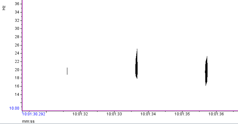
Based on what experts in the field of cetacean bioacoustics currently understand about fin whales, they produce sounds at a very low frequency for both socializing (presumably their 20 Hz pulse call) and for foraging (presumably their 40 Hz downsweep call) (Sirovic et al. 2013; Romagosa et al. 2021). During my efforts to determine the presence of fin whales, it is relatively easy to identify the 20 Hz pulse call, since this call has been well documented in the literature and is the only cetacean call described that occurs in its frequency range. I look for these calls in spectrogram representations of the acoustic data, which allow me to see the selected frequency range over our data collection period (time; Figure 1).

Figure 1. The two black vertical lines shown in this spectrogram are two 20 Hz fin whale pulse calls I identified in the HALO acoustic data using Raven Pro. Nearly all of the fin whale calls I’ve identified in the HALO data occur in pulses ranging from ~17 Hz to 27 Hz.   

Where this process becomes complicated for me is when I look for the 40 Hz fin whale downsweep call, which is known to occur between ~ 75 Hz – 30 Hz (Wiggins & Hildebrand 2020; Romagosa et al. 2021). This call can vary slightly within this frequency range. Interpretation of this call reaches even higher ambiguity when there are blue whales and sei whales acoustically detected in the same time frame in the same area. The acoustic repertoire of both blue and sei whale calls fall in the same frequency range: blue whales producing what is known as “D calls” and sei whales are known to make low-frequency downsweep calls (Figure 2; Sirovic et al. 2013; Romagosa et al. 2020).

Figure 2.  From left to right: Fin whale 40 Hz downsweep call (Sirovic et al. 2013); Blue whale D call, Sei whale downsweep call. (Romagosa et al. 2020)

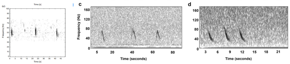
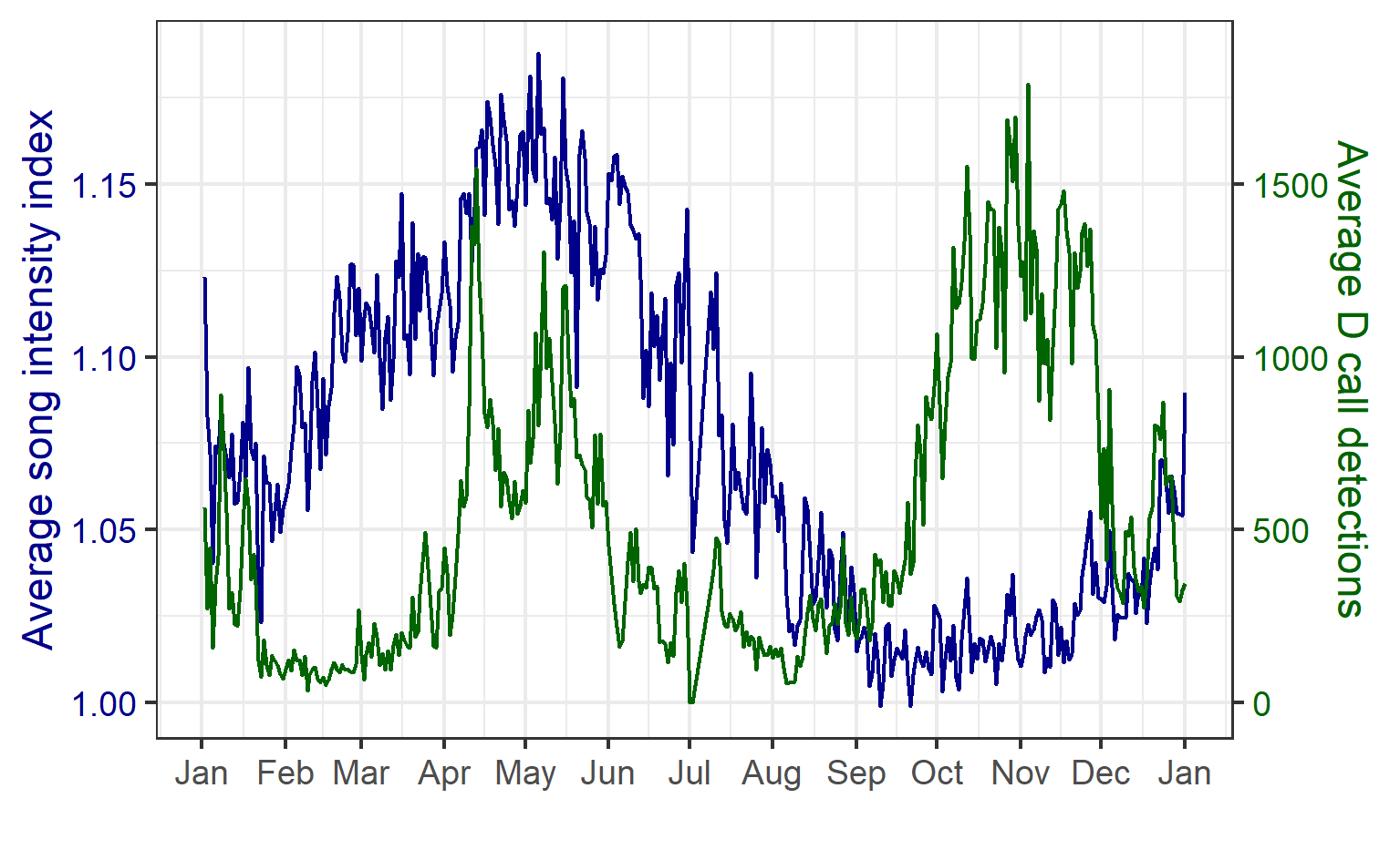
At first glance, the vocalizations from these three whales can be easily confused, and so I am looking for finer details to help tease out the fin whale downsweeps. As shown in Figure 2, there is a difference in the behavior of these calls, with the sei whale call being a shorter call by a matter of 2-3 seconds. The sei whale downsweep calls have not been frequently described in the literature, however those few publications report these calls occurring over 1.4-1.6 seconds (Baumgartner et al. 2008; Espanol-Jimenez et al. 2019) and in each published spectrogram, I have observed this similar boomerang-type looking behavior in the call. Blue whale D calls, on the other hand, are calls produced as social calls while foraging (Szesciorka et al 2020) and known to occur over ~1.8 seconds (Oleson et al. 2007).  

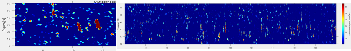
Fin whale 40 Hz calls have a duration of about one second and are not known to be produced in a regular sequence (Sirovic et al. 2013), thus I am teasing them out carefully from what can sometimes appear like a diversly grouped choir of low frequency whale song among the HALO data (Figures 3 & 4).  

Figure 3. Left hand figure: Red vertical lines occurring from 39 Hz to 22 Hz in the spectrogram are Fin whale 40 Hz call I have identified in the HALO data. Figure 4. Right hand figure shows many vertical lines in the 80 Hz to 20 Hz range that could be interpreted at first glance as different whale species vocalizations, including fin, blue and sei whales.

Although there are some known seasonal patterns of each of these aforementioned whale calls (Sirovic et al. 2013; Szesciorka et al. 2020), many data gaps remain of the temporal patterns of the 40 Hz and 20 Hz calls (i.e., when the calls occur) off the Oregon coast. Therefore, I cannot assume that I will only see 40 Hz calls in any time period. I need to assess the behavior of the calls I detect and tease out the calls I know surely are fin whale 40 Hz downsweeps in each file of the entire acoustic dataset.

Afterthought: The HALO project is new and has only just collected its first year of acoustic data, however the project is intent to continue deploying and collecting Rockhoppers off the Oregon coast for years to come. As this acoustic data set continues to grow it will be used by other researchers, and I (among the first to process and analyze it) feel some pressure to get things done right. As I process these data I will work hard to make the best-informed call identifying fin whales in the 40 Hz range. This focus and feeling of responsibility reassure me that I am in the appropriate career field. I really care about how these data are processed, where the research will go from here, and how it influences human activities in this critical whale habitat.

Photo credit: https://nextlevelsailing.com/how-big-is-a-whale-list-of-whales-by-size/

Did you enjoy this blog? Want to learn more about marine life, research, and conservation? Subscribe to our blog and get a weekly message when we post a new blog. Just add your name and email into the subscribe box below.

Loading

References

Baumgartner, M., Van Parijs, S., Wenzel, F., et al. 2008. Low frequency vocalizations attributed to sei whales. Acoustical Society of America, 124 (2): 1339-1349. https://www.whoi.edu/cms/files/JAS001339_59390.pdf.

Espanol-Jimenez, S., Bahamonde, P., Chiang, G., Haussermann, V. 2019. Discovering sounds in

Oleson, E., Calambokidis, J., Burgess, W,. et al. 2007. Behavioral context of call production by eastern North Pacific blue whales. Marine Ecology Progress Series, 330 : 269-284. https://www.int-res.com/articles/meps_oa/m330p269.pdf.

Romagosa, M., Baumgartner, M., Cascao, I., et al. 2020. Baleen whale acoustic presence and behavior at a Mid-Atlantic migratory habitat, the Azores Archipelago. Scientific Reports, 10. https://www.researchgate.net/publication/339952595_Baleen_whale_acoustic_presence_and_behaviour_at_a_Mid-Atlantic_migratory_habitat_the_Azores_Archipelago.

Romagosa, M., Perez-Jorge, S., Cascao, I., et al. 2021. Food talk: 40-Hz fin whale calls are associate with prey biomass. Proceedings of the Royal Society B: Biological Sciences, 288 (1954): 20211156. https://pubmed.ncbi.nlm.nih.gov/34229495/.

Sirovic, A., Williams, L., Kerosky, S., Wiggins, S., Hildebrand, J. 2013. Temporal separation of two fin whale call types across the eastern North Pacific. Marine Biology, 160: 47-57.

Szesciorka, A., Ballance, L., Sirovic, A., et al. 2020. Timing is everything: drivers of interannual variability in blue whale migration. Scientific Reports, 10 (7710). https://www.nature.com/articles/s41598-020-64855-y. Wiggins, S. & Hildebrand, J. 2020. Fin whale 40 Hz behavior studied with an acoustic tracking array. Marine Mammal Science, 36 (3). https://www.researchgate.net/publication/339575220_Fin_whale_40-Hz_calling_behavior_studied_with_an_acoustic_tracking_array.

Spreadsheets, ArcGIS, and Programming! Oh My!

By Morgan O’Rourke-Liggett, Master’s Student, Oregon State University, Department of Fisheries, Wildlife, and Conservation Sciences, Geospatial Ecology of Marine Megafauna Lab

Avid readers of the GEMM Lab blog and other scientists are familiar with the incredible amounts of data collected in the field and the informative figures displayed in our publications and posters. Some of the more time-consuming and tedious work hardly gets talked about because it’s the in-between stage of science and other fields. For this blog, I am highlighting some of the behind-the-scenes work that is the subject of my capstone project within the GRANITE project.

For those unfamiliar with the GRANITE project, this multifaceted and non-invasive research project evaluates how gray whales respond to chronic ambient and acute noise to inform regulatory decisions on noise thresholds (Figure 1). This project generates considerable data, often stored in separate Excel files. While this doesn’t immediately cause an issue, ongoing research projects like GRANITE and other long-term monitoring programs often need to refer to this data. Still, when scattered into separate long Excel files, it can make certain forms of analysis difficult and time-consuming. It requires considerable attention to detail, persistence, and acceptance of monotony. Today’s blog will dive into the not-so-glamorous side of science…data management and standardization!

Figure 1. Infographic for the GRANITE project. Credit: Carrie Ekeroth

Of the plethora of data collected from the GRANITE project, I work with the GPS trackline data from the R/V Ruby, environmental data recorded on the boat, gray whale sightings data, and survey summaries for each field day. These come to me as individual yearly spreadsheets, ranging from thirty entries to several thousand. The first goal with this data is to create a standardized survey effort conditions table. The second goal is to determine the survey distance from the trackline, using the visibility for each segment, and calculate the actual area surveyed for the segment and day. This blog doesn’t go into how the area is calculated. Still, all these steps are the foundation for finding that information so the survey area can be calculated.

The first step requires a quick run-through of the sighting data to ensure all dates are within the designated survey area by examining the sighting code. After the date is a three-letter code representing a different starting location for the survey, such as npo for Newport and dep for Depoe Bay. If any code doesn’t match the designated codes for the survey extent, those are hidden, so they are not used in the new table. From there, filling in the table begins (Figure 2).

Figure 2. A blank survey effort conditions table with each category listed at the top in bold.

Segments for each survey day were determined based on when the trackline data changed from transit to the sighting code (i.e., 190829_1 for August 29th, 2019, sighting 1). Transit indicated the research vessel was traveling along the coast, and crew members were surveying the area for whales. Each survey day’s GPS trackline and segment information were copied and saved into separate Excel workbook files. A specific R code would convert those files into NAD 1983 UTM Zone 10N northing and easting coordinates.

Those segments are uploaded into an ArcGIS database and mapped using the same UTM projection. The northing and easting points are imported into ArcGIS Pro as XY tables. Using various geoprocessing and editing tools, each segmented trackline for the day is created, and each line is split wherever there was trackline overlap or U shape in the trackline that causes the observation area to overlap. This splitting ensures the visibility buffer accounts for the overlap (Figure 3).

Figure 3. Segment 3 from 7/22/2019 with the visibility of 3 km portrayed as buffers. There are more than one because the trackline was split to account for the overlapping of the survey area. This approach accounts for the fact that this area where all three buffers overlap was surveyed 3 times.

Once the segment lines are created in ArcGIS, the survey area map (Figure 4) is used alongside the ArcGIS display to determine the start and end locations. An essential part of the standardization process is using the annotated locations in Figure 4 instead of the names on the basemap for the location start and endpoints. This consistency with the survey area map is both for tracking the locations through time and for the crew on the research vessel to recognize the locations. The step assists with interpreting the survey notes for conditions at the different segments. The time starts and ends, and the latitude and longitude start and end are taken from the trackline data.

Figure 4. Map of the survey area with annotated locations (Created by L. Torres, GEMM Lab)

The sighting data includes the number of whales sighted, Beaufort Sea State, and swell height for the locations where whales were spotted. The environmental data from the sighting data is used as a guide when filling in the rest of the values along the trackline. When data, such as wind speed, swell height, or survey condition, is not explicitly given, matrices have been developed in collaboration with Dr. Leigh Torres to fill in the gaps in the data. These matrices and protocols for filling in the final conditions log are important tools for standardizing the environmental and condition data.

The final product for the survey conditions table is the output of all the code and matrices (Figure 5). The creation of this table will allow for accurate calculation of survey effort on each day, month, and year of the GRANITE project. This effort data is critical to evaluate trends in whale distribution, habitat use, and exposure to disturbances or threats.

Figure 5. A snippet of the completed 2019 season effort condition log.

The process of completing the table can be a very monotonous task, and there are several chances for the data to get misplaced or missed entirely. Attention to detail is a critical aspect of this project. Standardizing the GRANITE data is essential because it allows for consistency over the years and across platforms. In describing this aspect of my project, I mentioned three different computer programs using the same data. This behind-the-scenes work of creating and maintaining data standardization is critical for all projects, especially long-term research such as the GRANITE project.

Did you enjoy this blog? Want to learn more about marine life, research, and conservation? Subscribe to our blog and get a weekly message when we post a new blog. Just add your name and email into the subscribe box below.

Loading

So big, but so small: why the smallest of the largest whales are not smaller

Dr. KC Bierlich, Postdoctoral Scholar, OSU Department of Fisheries, Wildlife, & Conservation Sciences, Geospatial Ecology of Marine Megafauna (GEMM) Lab

Baleen whales are known for their gigantism and encompass a wide range in body sizes extending from blue whales that are the largest animals to live on earth (max length ~30 m) to minke whales (max length ~10 m) that are the smallest of baleen whales (Fig. 1). While all baleen whales are filter feeders, a group called the rorquals use a feeding strategy known as lunge feeding (or intermittent engulfment filtration), which involves engulfing large volumes of prey-laden water at high speeds and then filtering the water out of their mouth using their baleen as a “sieve”. There is positive allometry associated with this feeding technique and body size, meaning that as whales are larger, this feeding strategy becomes more efficient due to increased engulfment of water volume per each lunge feeding event. In other words, a bigger body size equates to a much larger mouthful of food. For example, a minke whale (body length ~7-10 m) will engulf water volume equivalent to ~42% of its body mass, while a blue whale (~21-24 m) engulfs ~135%. Thus, filter feeding enables gigantism through efficient exploitation of large, dense patches of prey. An interesting question then arises: what is the minimum body size at which filter feeding is still efficient? Or in other words, why are the smallest of the baleen whales, minke whales, not smaller? For this blog, I will highlight a study published today in Nature Ecology and Evolution titled “Minke whale feeding rate limitations suggest constraints on the minimum body size for engulfment filtration feeding” led by friend and collaborator of the GEMM Lab Dr. Dave Cade and included myself and other collaborators as co-authors from Stanford University, UC Santa Cruz, Cascadia Research Collective, Duke University, and University of Queensland.

Figure 1. Aerial imagery collected using drones of several baleen whales of various sizes. Each species shown is considered a rorqual whale, except for gray whales. Figure from Segre et al. (2022)

The largest animals of today are marine filter feeders, such as whale sharks, manta rays, and baleen whales, which all share parallel evolutionary histories in which their large body sizes and filter-feeding morphologies are derived from smaller-bodied ancestors that targeted single prey items. Changes in ocean productivity increased the concentrations of smaller prey in the oceans around 5 million years ago, enabling filter feeding as an efficient feeding strategy through capture of abundant aggregations of prey by filtering large volumes of water. It is interesting to note, that within these filter feeding lineages of animals, there are groups of animals that are single-prey foragers with smaller body sizes. For example, the whale shark is the only filter feeder amongst the carpet sharks and the manta ray is much larger than other rays that feed on single prey items. Amongst cetaceans, the smallest single-prey foragers, dolphins (~2-3 m) and porpoises (~1.4-1.9 m), are much smaller than the smallest of the filter feeding cetaceans, minke whales (~7-10 m). These common differences in body sizes and feeding strategies within lineages suggest that there may be minimum body size requirements for this filter feeding strategy to be efficient.

To investigate the limits on minimum body size for filter feeding, our study explored the foraging behavior of Antarctic minke whales, the smallest of the rorqual baleen whales, along the Western Antarctic Peninsula. Our team tagged a total of 23 individuals using non-invasive suction cup tags, like the ones we use for our tagging component in the GEMM Lab’s GRANITE project (see this blog for more details). One of my roles on the project was to obtain aerial imagery of the minke whales using drones to obtain body length measurements (sound familiar?) (Figs. 2-4). Flying drones in Antarctica over minke whales was an amazing experience. The minke whales were often found deep within the bays amongst ice floes and brash ice where they can be very tricky to spot, as they’ll often surface and then quickly disappear, hence their nickname “sneaky minkes”. They also appear “playful” and “athletic” as they are incredibly quick and maneuverable, doing barrel rolls and quick bank turns while they swim. Check out my past blog to read more on accounts of flying over these amazing whales.

Figure 2. Drone image of our team about to place a noninvasive suction cup biologging tag on an Antarctic minke whale. Photo credit: Duke University Marine Robotics and Remote Sensing Lab.
Figure 3. A drone image of a newly tagged and curious Antarctic minke whale approaching our research team. Photo credit: Duke University Marine Robotics and Remote Sensing Lab.
Figure 4. A drone image of a group of Antarctic minke whales swimming through the icy waters along the Antarctic Peninsula. Photo credit: Duke University Marine Robotics and Remote Sensing Lab.

In total, our team collected 437 hours of tag data consisting of day- and night-time foraging behaviors. While the proportion of time spent foraging and the number of lunges per dive (~3-4) was similar between day- and night-time foraging, daytime foraging was much deeper (~72 m) compared to nighttime foraging (~28 m) due to vertical migration of Antarctic krill, their main food source. Overall, nighttime foraging was much more intense than daytime foraging, with an average of 165 lunges per hour during the night compared to 53 lunges per hour during the day. These shallower nighttime dives enabled quicker surface sequences for replenishing oxygen reserves to then return to foraging, whereas the deeper dives during the day required longer surface recovery times before beginning another foraging dive. Thus, nighttime dives are a more efficient and critical component of minke whale foraging.

When it comes to body size, there was no relationship between dive depth and dive duration with body length, except for daytime deep dives, where longer minke whales dove for longer periods than smaller whales. These longer dive times also require longer surface times to replenish oxygen reserves. Longer minke whales can gulp larger amounts of food and thus need longer filtration times to process water from each engulfment. For example, a 9 m minke whale will take 50% longer to filter water through its baleen compared to a 5 m minke whale. In turn, smaller minke whales would need to feed more frequently than larger minke whales in order to maintain efficient foraging. This decreasing efficiency with smaller body size shines light on a broader trend for filter feeders that we refer to in our study as the minimum-size constraint (MSC) hypothesis: “while the maximum size of a filter-feeding body plan will be restricted by physical properties, the minimum size is restricted by the energetic efficiency of filter feeding and the time required to extract sufficient particles from the water” (Cade et al. 2023). When we examined the scaling of maximum feeding rates of minke whales, we found evidence of a minimum size constraint on efficiency at lengths around 5 m. Interestingly, the weaning length of minke whales is reported to be 4.5 – 5.5 m. Before weaning, newborn/yearling minke whales that are smaller than 4.5 ­– 5.5 m have a different foraging strategy where they are dependent on maternal milk. Thus, it is likely that the body size at weaning is influenced by the minimum size at which this specialized foraging technique of lunge feeding becomes efficient.

This study helps inform the evolutionary pathway for filter feeding whales and suggests that efficient filter feeding and gigantism likely co-evolved within the last 5 million years when ocean conditions changed to support larger prey patches suitable for lunge feeding. It is interesting to think about the MSC hypothesis for other baleen whale species that employ alternative filter feeding techniques, such as gray whales that generally use a form of filter feeding called suction feeding. Gray whales are estimated to have a birth length of ~4.6 m (Agbayani et al., 2020), and the body length of newly weaned calves that we have observed along the Oregon Coast from drone imagery seem to be ~8 – 9 m. Perhaps this is the minimum size of when suction feeding becomes efficient for a gray whale? This is something the GEMM Lab hopes to further explore as we continue to collect foraging data from suction cup tags and behavior and body size measurements from drone imagery.

References

Agbayani, S., Fortune, S. M., & Trites, A. W. (2020). Growth and development of North Pacific gray whales (Eschrichtius robustus). Journal of Mammalogy101(3), 742-754.

Cade, D.E., Kahane-Rapport, S.R., Gough, W.T., Bierlich, K.C., Linksy, J.M.J., Johnston, D.W., Goldbogen, J.A., Friedlaender, A.S. (2023). Ultra-high feeding rates of Antarctic minke whales imply a lower limit for body size in engulfment filtration feeders. Nature Ecology and Evolution. https://www.nature.com/articles/s41559-023-01993-2  

Paolo S. Segre, William T. Gough, Edward A. Roualdes, David E. Cade, Max F. Czapanskiy, James Fahlbusch, Shirel R. Kahane-Rapport, William K. Oestreich, Lars Bejder, K. C. Bierlich, Julia A. Burrows, John Calambokidis, Ellen M. Chenoweth, Jacopo di Clemente, John W. Durban, Holly Fearnbach, Frank E. Fish, Ari S. Friedlaender, Peter Hegelund, David W. Johnston, Douglas P. Nowacek, Machiel G. Oudejans, Gwenith S. Penry, Jean Potvin, Malene Simon, Andrew Stanworth, Janice M. Straley, Andrew Szabo, Simone K. A. Videsen, Fleur Visser, Caroline R. Weir, David N. Wiley, Jeremy A. Goldbogen; Scaling of maneuvering performance in baleen whales: larger whales outperform expectations. J Exp Biol 1 March 2022; 225 (5): jeb243224. doi: https://doi.org/10.1242/jeb.243224

Learning by teaching

By: Kate Colson, MSc Student, University of British Columbia, Institute for the Oceans and Fisheries, Marine Mammal Research Unit

One of the most frequent questions graduate students get asked (besides when you are going to graduate) is what their plans are after university. For me, the answer has always adamantly been continuing to do research, most likely as a government researcher because I don’t want teaching commitments to take away from my ability to conduct research.

However, one of the most fulfilling parts of my degree at University of British Columbia has actually been teaching four terms of a 100-level undergraduate science course focused on developing first-year students’ critical thinking, data interpretation, and science communication skills. My role in the course has been facilitating active learning activities that exercise these skills and reviewing material the students go over in their pre-class work. Through this course, I have experienced the teaching styles of six different professors and practiced my own teaching. As with any skill, there is always room for improvement, so when I had a chance to read a book titled How Learning Works: Seven Research-Based Principles for Smart Teaching (Ambrose et al. 2010), I took it as an opportunity to further refine my teaching and explore why some practices are more effective than others.

In the book, Ambrose et al. present principles of learning, the research surrounding these principles and examples for incorporating them into a university level course. Some of the principles gave me ideas for strategies to incorporate into my teaching to benefit my students. These described how prior knowledge impacts student learning and how to use goal-oriented practice and give feedback relative to target criteria that the students can apply to the next practice task. For example, I learned to be more conscious about how I explain and clarify course material to make connections with what the students have learned previously, so they can draw on that prior knowledge. Other principles presented by Ambrose et al. were more complex and offered a chance for greater reflection.

Beyond presenting strategies for improving teaching, the book also presented research that supported what I had learned firsthand through teaching. These principles related to the factors that motivate students to learn and why the course climate matters for learning. I have seen how student motivation is impacted by the classroom climate and culture put forth by the teaching team. Perhaps the most frustrating experiences I have had teaching were when one member of the teaching team does not see the importance of fostering a supportive course environment.

For this reason, my favorite assignments have been the Thrive Contract and the Group Contract. Each term, the Thrive Contract is the first major class activity, and the Group Contract is the first group assignment. These assignments serve as a means for everyone to co-create guidelines and expectations and establish a positive classroom culture for the rest of the term. After an exceptionally poor classroom experience my first time teaching, I have highlighted the importance of the Thrive Contract in all subsequent terms. Now, I realize the significance I lent this assignment is supported by the research on the importance for a supportive environment to maximize student motivation and encourage classroom engagement (Figure 1).

Another powerful lesson I have learned through teaching is the importance of clarifying the purpose of an activity to the students. Highlighting a task’s objective is also supported by research to ensure that students ascribe value to the assigned work, increasing their motivation (Figure 1).  In my teaching, I have noticed a trend of lower student participation and poorer performance on assignments when a professor does not emphasize the importance of the task. Reviewing the research that shows the value of a supportive course climate has further strengthened my belief in the importance of ensuring that students understand why their teaching team assigns each activity.

Figure 1. How environment, student efficacy, and value interact to impact motivation. The above figure shows that motivation is optimized when students see the value in a goal, believe they have the skills to achieve the goal, and are undertaking the goal in a supportive class environment (the bright blue box in the bottom right corner). If this situation were to occur in an unsupportive class environment, defiant behaviour (e.g. “I’ll prove you wrong” attitude) is likely to occur in response to the lack of support, as the student sees the value in the goal and believes in their ability to achieve the goal. Rejecting behaviour (e.g., disengagement) occurs when the student does not associate value to a task and does not believe in their ability to complete the goals regardless of the environment.  Evading behaviour (e.g., lack of attention or minimal effort) results when students are confident in their ability to complete a task, but do not see the goal as meaningful in both supportive and unsupportive environment. When a student sees the importance of the goal but are not confident in their ability to complete it, they become hopeless (e.g., have no expectation of success and act helpless) when in an unsupportive environment and fragile (e.g., feign understanding, deny difficulty, or make excuses for poor performance) in a supportive environment.  Diagram adapted from Ambrose et al. (2010) Figure 3.2 incorporating the works of Hansen (1989) & Ford (1992).

Potentially my favorite part about the structure of Ambrose’s book was that it offered me a chance to reflect not only on teaching, but also on my own learning and cognitive growth since I started my master’s degree. Graduate students are often in a unique position in which we are both students and teachers depending on the context of our surroundings. The ability to zoom out and realize how far I have come in not only teaching others, but also in teaching myself, has been humbling. My reflection on my own learning and growth has been driven by learning about how organizing knowledge affects learning, how mastery is developed and how students become self-directed learners.

One of the main differences between novices and experts in how they organize their knowledge is the depth of that knowledge and the connections made between different pieces of information. Research has shown that experts hold more connections between concepts, which allows for faster and easier retrieval of information that translates into ease in applying skills to different tasks (Bradshaw & Anderson, 1982; Reder & Anderson, 1980; Smith, Adams, & Schorr, 1978). Currently in my degree, I am experiencing this ease when it comes to coding my analysis and connecting my research to the broader implications for the field. By making these deeper connections across various contexts, I am building a more complex knowledge structure, thus progressing towards holding a more expert organization of knowledge.

In the stages of mastery concept proposed by Sprague and Stewart (2000), learners progress from unconscious incompetence where the student doesn’t know what they don’t know, to conscious incompetence where they have become aware of what they need to know (Figure 2). This was where I was when I started my master’s — I knew what objectives I wanted to achieve with my research, but I needed to learn the skills necessary for me to be able to collect the data and analyze it to answer my research questions. The next stage of mastery is conscious competence, in which the ability of the learner to function in their domain has greatly increased, but practicing the necessary skills still requires deliberate thinking and conscious actions (Figure 2). This is the level I feel I have progressed to — I am much more comfortable performing the necessary tasks related to my research and talking about how my work fills existing knowledge gaps in the field. However, it still helps to talk out my proposed plans with true masters in the field. The final stage of mastery, unconscious competence, is where the learner has reached a point where they can practice the skills of their field automatically and instinctively such that they are no longer aware of how they enact their knowledge (Figure 2).

Figure 2. Stages of mastery showing how the learner consciousness waxes and then wanes as competence is developed. Unconscious states refer to those where the learner is not aware of what they are doing or what they know, whereas conscious states have awareness of thoughts and actions. Competence refers to the ability of the learner to perform tasks specific to the field they are trying to master. Diagram adapted from Ambrose et al. (2010) Figure 4.2 incorporating the works of Sprague & Stewart (2000).

In line with my progression to higher levels of mastery has come the development of metacognitive skills that have helped me become a better self-directed learner. Metacognition is the process of learning how to learn, requiring the learner to monitor and control their learning through various processes (Figure 3). The most exciting part of my metacognitive growth I have noticed is the greater independence I have in my learning. I am much better at assessing what is needed to complete specific tasks and planning my particular approach to successfully achieve that goal (e.g., the construction of a Hidden Markov model from my last blog). By becoming more aware of my own strengths and weaknesses as a learner, I am better able to prepare and give myself the support needed for completing certain tasks (e.g., reaching out to experts to help with my model construction as I knew this was an area of weakness for me). By becoming more aware of how I am monitoring and controlling my learning, I know I am setting myself up for success as a lifelong learner.

Figure 3. Metacognition requires learner to monitor and control their learning through various processes. These processes involve the learner assessing the necessary skills needed for a task, evaluating their strengths and weaknesses with regards to the assigned task, and planning a way to approach the task. Once a plan has been made, the learner then must apply the strategies involved from the plan and monitor how those strategies are working to accomplish the assigned task. The learner must then be able to decide if the planned approach and applied strategies are effectively accomplishing the assigned task and adjust as needed with a re-assessment of the task that begins the processing cycle over again. Underlying each of these metacognitive processes are the learner’s belief in their own abilities and their perceptions of their intelligence. For example, students who believe their intelligence cannot be improved and do not have a strong sense of efficacy will be less likely to expend effort in metacognitive processes as they believe the extra effort will not influence the results. This contrasts with students who believe their intelligence will increase with skills development and have a strong belief in their abilities, as these learners will see the value in putting in the effort of trying multiple plans and adjusting strategies.  Diagram adapted from Ambrose et al. (2010) Figure 7.1 incorporating the cycle of adaptive learning proposed by Zimmerman (2001).
Loading

References:

Ambrose, S. A., Bridges, M. W., DiPietro, M., Lovett, M. C., & Norman, M. K. (2010). How learning works: Seven research-based principles for smart teaching (1st ed.). San Francisco, CA: Jossey-Bass. 

Bradshaw, G. L., & Anderson, J. R. (1982). Elaborative encoding as an explanation of levels of processing. Journal of Verbal Learning and Verbal behaviours, 21,165-174.

Ford, M. E. (1992). Motivating humans: Goals, emotions and personal agency beliefs. Newbury Park, CA: Sage Publications, Inc.

Hansen, D. (1989). Lesson evading and dissembling: Ego strategies in the classroom. American Journal of Education, 97, 184-208.

Reder, L. M., & Anderson, J. R. (1980). A partial resolution of the paradox of interference: The role of integrating knowledge.  Cognitive Psychology, 12,  447-472.

Smith, E. E., Adams, N., & Schorr, D. (1978). Fact retrieval and the paradox of interference. Cognitive Psychology, 10, 438-464.

Sprague, J., & Stewart, D. (2000). The speaker’s handbook. Fort Worth, TX: Harcourt College Publishers.

Zimmerman, B. J. (2001). Theories of self-regulated learning and academic achievement: An overview and analysis. In B. J. Zimmerman & D. H. Schunk (Eds.), Self-regulated learning and academic achievement (2nd ed., pp. 1-38). Hillsdale, NJ: Erlbaum.

New GEMM Lab publication reveals how blue whale feeding and reproductive effort are related to environmental conditions

By Dr. Dawn Barlow, Postdoctoral Scholar, OSU Department of Fisheries, Wildlife, and Conservation Sciences, Geospatial Ecology of Marine Megafauna Lab

Learning by listening

Studying mobile marine animals that are only fleetingly visible from the water’s surface is challenging. However, many species including baleen whales rely on sound as a primary form of communication, producing different vocalizations related to their fundamental needs to feed and reproduce. Therefore, we can learn a lot about these elusive animals by monitoring the patterns of their calls. In the final chapter of my PhD, we set out to study blue whale ecology and life history by listening. I am excited to share our findings, recently published in Ecology and Evolution.

Blue whales produce two distinct types of vocalizations: song is produced by males and is hypothesized to play a role in breeding behavior, and D calls are a hypothesized social call produced by both sexes in association with feeding behavior. We analyzed how these different calls varied seasonally, and how they related to environmental conditions.

This paper is a collaborative study co-authored by Dr. Holger Klinck and Dimitri Ponirakis of the K. Lisa Yang Center for Conservation Bioacoustics, Dr. Trevor Branch of the University of Washington, and GEMM Lab PI Dr. Leigh Torres, and brings together multiple methods and data sources. Our findings shed light on blue whale habitat use patterns, and how climate change may impact both feeding and reproduction for this species of conservation concern.

The South Taranaki Bight: an ideal study system

Baleen whales typically migrate between high-latitude, productive feeding grounds and low-latitude breeding grounds. However, the New Zealand blue whale population is present in the South Taranaki Bight (STB) region year-round, which uniquely enabled us to monitor their behavior, ecology, and life history across seasons and years from a single location. We recorded blue whale vocalizations from Marine Autonomous Recording Units (MARUs) deployed at five locations in the STB for two full years (Fig. 1).

Figure 1. Study area map and blue whale call spectrograms. Left panel: map of the study area in the South Taranaki Bight region, with hydrophone (marine autonomous recording unit; MARU) locations denoted by the stars. Gray lines show bathymetry contours at 50 m depth increments, from 0 to 500 m. Location of the study area within New Zealand is indicated by the inset map. Right panels: example spectrograms of the two blue whale call types examined: the New Zealand song recorded on 31 May 2016 (top) and D calls recorded 20 September 2016 (bottom). Figure reproduced from Barlow et al. (2023).

We found that the two vocalization types had different seasonal occurrence patterns (Fig. 2). D calls were associated with upwelling conditions that indicate feeding opportunities, lending evidence for their function as a foraging-related call.

Figure 2. Average annual cycle in the song intensity index (dark blue) and D calls (green) per day of the year, computed across all hydrophone locations and the entire two-year recording period. Figure reproduced from Barlow et al. (2023).

In contrast, blue whale song showed a very clear seasonal peak in the fall and was less obviously correlated with environmental conditions. To investigate the hypothesized function of song as a breeding call, we turned to a perhaps unintuitive source of information: historical whaling records. Whenever a pregnant whale was killed during commercial whaling operations, the length of the fetus was measured. By looking at the seasonal pattern in these fetal lengths, we can presume that births occur around the time of year when fetal lengths are at their longest. The records indicated April-May. By back-calculating the 11-month gestation time for a blue whale, we can presume that mating occurs generally in May-June, which is the exact time of the peak in song intensity from our recordings (Fig. 3).

Figure 3. Annual song intensity and the breeding cycle. Top panel: average yearly cycle in song intensity index, computed across the five hydrophone locations and the entire recording period; dark blue line represents a loess smoothed fit. Bottom panel: fetal length measurements from whaling catch records for Antarctic blue whales (gray, measurements rounded to the nearest foot), pygmy blue whales in the southern hemisphere (blue, measurements rounded to the nearest centimeter). Measurements from blue whales caught within the established range of the New Zealand population are denoted by the dark red triangles. Calving presumably takes place around or shortly after fetal lengths are at their maximum (April–May), which implies that mating likely occurs around May–June, coincident with the peak song intensity. Figure reproduced from Barlow et al. (2023).

With this evidence for D calls as feeding-related calls and song as breeding-related calls, we had a host of new questions, we used this gained knowledge to explore how changing environmental conditions might impact multiple life history processes for New Zealand blue whales

Marine heatwaves impact multiple life history processes

Our study period between January 2016 and February 2018 spanned both typical upwelling conditions and dramatic marine heatwaves in the STB region. While we previously documented that the marine heatwave of 2016 affected blue whale distribution, the population-level impacts on feeding and reproductive effort remained unknown. In our recent study, we found that during marine heatwaves, D calls were dramatically reduced compared to during productive upwelling conditions. During the fall breeding peak, song intensity was likewise dramatically reduced following the marine heatwave. This relationship indicates that following poor feeding conditions, blue whales may invest less effort in reproduction. As marine heatwaves are projected to become more frequent and more intense under global climate change, our findings are perhaps a warning for what is to come as animal populations must contend with changing ocean conditions.

More than a decade of research on New Zealand blue whales

Ten years ago, Leigh first put forward a hypothesis that the STB region was an undocumented blue whale foraging ground based on multiple lines of evidence (Torres 2013). Despite pushback and numerous challenges, Leigh set out to prove her hypothesis through a comprehensive, multi-year data collection effort. I was lucky enough to join the team in 2016, first as a Masters’ student, and then as a PhD student. In the time since Leigh’s hypothesis, we not only documented the New Zealand blue whale population (Barlow et al. 2018), we learned a great deal about what drives blue whale feeding behavior (Torres et al. 2020) and habitat use patterns (Barlow et al. 2020, 2021), and developed forecast models to predict blue whale distribution for dynamic management of the STB (Barlow & Torres 2021). We also documented their unique, year-round presence in the STB, distinct from the migratory or vagrant presence of other blue whale populations (Barlow et al. 2022b). We now understand how marine heatwaves impact both feeding opportunities and reproductive effort (Barlow et al. 2023). We even analyzed blue whale skin condition (Barlow et al. 2019) and acoustic response to earthquakes (Barlow et al. 2022a) along the way. A decade later, it is humbling to reflect on how much we have learned about these whales. This paper is also the final chapter of my PhD, and as I reflect on how I have grown both personally and scientifically since I interviewed with Leigh as a wide-eyed undergraduate student in fall 2015, I am filled with gratitude for the opportunities for learning and growth that Leigh, these whales, and many mentors and collaborators have offered over the years. As is often the case in science, the more questions you ask, the more questions you end up with. We are already dreaming up future studies to further understand the ecology, health, and resilience of this blue whale population. I can only imagine what we might learn in another decade.

Figure 5. A blue whale mother and calf pair come up for air in the South Taranaki Bight. Photo by Dawn Barlow.

Did you enjoy this blog? Want to learn more about marine life, research, and conservation? Subscribe to our blog and get a weekly alert when we make a new post! Just add your name into the subscribe box below!

Loading

References:

Barlow DR, Bernard KS, Escobar-Flores P, Palacios DM, Torres LG (2020) Links in the trophic chain: Modeling functional relationships between in situ oceanography, krill, and blue whale distribution under different oceanographic regimes. Mar Ecol Prog Ser 642:207–225.

Barlow DR, Estrada Jorge M, Klinck H, Torres LG (2022a) Shaken, not stirred: blue whales show no acoustic response to earthquake events. R Soc Open Sci 9:220242.

Barlow DR, Klinck H, Ponirakis D, Branch TA, Torres LG (2023) Environmental conditions and marine heatwaves influence blue whale foraging and reproductive effort. Ecol Evol 13:e9770.

Barlow DR, Klinck H, Ponirakis D, Garvey C, Torres LG (2021) Temporal and spatial lags between wind, coastal upwelling, and blue whale occurrence. Sci Rep 11:1–10.

Barlow DR, Klinck H, Ponirakis D, Holt Colberg M, Torres LG (2022b) Temporal occurrence of three blue whale populations in New Zealand waters from passive acoustic monitoring. J Mammal.

Barlow DR, Pepper AL, Torres LG (2019) Skin deep: An assessment of New Zealand blue whale skin condition. Front Mar Sci 6:757.

Barlow DR, Torres LG (2021) Planning ahead: Dynamic models forecast blue whale distribution with applications for spatial management. J Appl Ecol 58:2493–2504.

Barlow DR, Torres LG, Hodge KB, Steel D, Baker CS, Chandler TE, Bott N, Constantine R, Double MC, Gill P, Glasgow D, Hamner RM, Lilley C, Ogle M, Olson PA, Peters C, Stockin KA, Tessaglia-hymes CT, Klinck H (2018) Documentation of a New Zealand blue whale population based on multiple lines of evidence. Endanger Species Res 36:27–40.

Torres LG (2013) Evidence for an unrecognised blue whale foraging ground in New Zealand. New Zeal J Mar Freshw Res 47:235–248.

Torres LG, Barlow DR, Chandler TE, Burnett JD (2020) Insight into the kinematics of blue whale surface foraging through drone observations and prey data. PeerJ 8:e8906.

Immersive Marine Science: Diving for Data and a New Perspective on Gray Whale Habitat

Allison Dawn, GEMM Lab Master’s student, OSU Department of Fisheries, Wildlife and Conservation Sciences, Geospatial Ecology of Marine Megafauna Lab 

If you have followed the GEMM Lab blog for a while, you have read about the multitude of techniques we use to conduct research. A combination of platforms and technologies help us observe whales: rigid inflatable boats (RHIBs), kayaks, theodolites, cameras, binoculars, high-tech drones, and more. However, not only do we observe from the sky and sea surface, but we also know it is important to monitor whale behavior, habitat, and prey underwater. For this week’s blog, I’d like to highlight the GEMM Lab’s sub-surface efforts as part of the TOPAZ/JASPER project, and share more about the world of scientific diving.

Most terrestrial ecologists have the luxury of strolling through their study systems without having to give thought to their next breath, but marine scientists need creative, streamlined, and most importantly, life-preserving ways to directly observe the ocean environment. Like most inventions, today’s self-contained underwater breathing apparatus (SCUBA) equipment was developed from countless prototypes worldwide, dating as far back as the 1800s. This equipment was improved during World War II, specifically to support combat swimmers (called “frogmen” at the time). After the Franco-German Armistice of 1940, French engineer Émile Gagnan and Naval Lieutenant/Oceanographer Jacques Cousteau teamed up to invent the “Aqua-Lung” (Fig. 1), which allowed divers to autonomously stay underwater for much longer periods of time. 

Figure 1: Vintage advertisement for the Aqua-Lung (left) and a diver testing out the equipment (right). Photos sourced from https://us.aqualung.com/en/ourstory.html

Now that the first commercially successful breathing apparatus was available, universities began to purchase these units to aid with scientific exploration. However, after a series of fatal diving accidents, the Scripps Institution of Oceanography felt it was urgent to develop the first scientific diving safety program in 1954, years before recreational diving courses were implemented. With specific tasks at hand, the additional level of distraction makes safety and situational awareness that much more important. Now, scientific dive programs, like the one at OSU, are widespread, and after proper safety precautions and training, researchers have been able to accomplish what was previously implausible: restore coral reefs, obtain genetic information from invasive species, monitor species under polar ice sheets, and so much more (Fig. 2).

Figure 2: Scientific divers at work. Norwegian polar ice diver Michal Tessman collects algae, zooplankton, and phytoplankton samples (left); Florida State doctoral student Nathan Spindel obtains genetic material from urchins (top right); Dr. Colleen Bove of UNC Chapel Hill monitors tropical coral growth (bottom right).

On the south coast of Oregon, the GEMM lab collaborates with Dr. Aaron Galloway, an accomplished scientific diver and one of the lead scientists with the Oregon Kelp Alliance (ORKA), an organization dedicated to kelp forest monitoring, urchin culling, and restoration efforts. He and his team, along with our long-term project partner Dave Lacey of South Coast Tours, help us deploy our in situ underwater cameras each summer (Figs 3 & 4). As you may know, the TOPAZ component of our project aims to link fine-scale gray whale foraging ecology to prey distribution patterns, using inexpensive field methods. The in situ underwater CamDO camera systems are an exciting, recent addition to our long-standing sampling approach.

Figure 3: CamDo lander with attached oceanographic sensors (left); two new OSU scientific divers and Marine Studies Initiative interns, Faith Townsend and Caroline Rice, preparing to dive (right).

We have two durable camera housings that anchor in Mill Rocks and Tichenor Cove. In each housing we insert a GoPro, an extra battery, and a microcontroller programmed to record footage at continuous intervals. With these cameras we capture hundreds of hours of underwater footage of fish, zooplankton, and we hope to one day record gray whale foraging.

Figure 4: Dr. Aaron Galloway and his graduate student Samantha Persad getting ready to complete the final dive of the season in ideal visibility conditions.

Each week during the field season, the divers and I meet early at the dock to board the tour boat Black Pearl for our routine CamDO maintenance excursions. My first role on the early morning journeys is to be a “dive tender” — I help the divers back on board, log their dive times and air pressure, and keep gear organized on the boat. Then, while the divers relax and enjoy a snack, my next role begins. The next few minutes is what we refer to as the “NASCAR pit-stop” of camera maintenance: I replace batteries, swap SD cards, program the camera, ensure that it is secure in the housing, and tuck it into the diver’s bag along with installation tools. All the while, I simultaneously listen for radio calls from our Port Orford interns, sometimes troubleshooting urgent questions while they collect zooplankton and water quality data from the kayak or observe for whales from the cliff.

This multitasking is challenging, but at least I am dry, warm, and have total dexterity of my hands. As I watch the divers descend, in all their neoprene glory, to secure the camera back to its stationary landing, I like to imagine what they are seeing and experiencing. If visibility is good, they will descend into a cerulean blue world filled with rockfish, jellies, mysid swarms, and algae covered reefs (Fig 5.). However, as exciting as sightseeing can be while diving, my own scientific diver training has allowed me to understand the focus, determination, and adaptability even the simplest of tasks require, especially in the chilly waters of the Pacific Northwest.

Figure 5: Under the surface: black rockfish enjoying a swim around the rocky reefs in Tichenor Cove, Port Orford.

I earned my AAUS Scientific Diver certification in 2018 through UNC Chapel Hill, and have since learned just how different cold water is from warm water diving. My first cold water dive was at the Orford Reef exhibit in the Oregon Coast Aquarium. Guided by Kevin Buch, OSU’s Diving and Boat Safety Officer, I gained a new respect for how important it is to train in the conditions you will be working in. For example, cold-water diving requires much more insulation, which in turn changes your buoyancy and dexterity. At first, I struggled to learn my new buoyancy baseline while simultaneously rolling out transect tape with thick neoprene gloves and keeping a curious sturgeon from stealing my mask. At times it felt like I was learning to dive all over again. This winter, I have increased my confidence by taking evening SCUBA proficiency courses to sharpen my skills and logging dives in local conditions.

Figure 6: Obtaining my open water certification on the French Reef in Florida Keys, 2018.

As part of our Advanced Diver weekend course in the beautiful Hood Canal, I had the opportunity to hone my skills in compass navigation, buoyancy, night and deep dives, and search & recovery methods, all in my new cold water gear. While my dive buddy and I were ecstatic to see some amazing flora and fauna (giant pacific octopus, sea pens, nudibranch, pipefish, and more!) we mainly bonded over the shared sense of achievement in safely completing our complex tasks in low-visibility, cold-water conditions.

Figure 7: Giant Pacific Octopus like this can be observed while diving in the Hood Canal, photo credit Bruce Kerwin.

As I complete these trainings, I think of all there is to to be discovered with data collected under the surface of our Port Orford study system: the health of kelp forests, the density and patchiness of mysid shrimp (the crucial prey source for gray whales), habitat complexity, and more. I am curious if there are certain puzzle pieces driving gray whale foraging decisions that may be revealed through expanding our subsurface monitoring efforts as part of the GEMM Lab’s already impressive dataset.

The skill sets required for scientific diving are also useful for outdoor leadership, and truly in all situations: maintaining a cool head under stressful conditions, planning for the unexpected, managing expectations, and communicating well (you can’t really talk with a regulator in your mouth!) — to name just a few. Regardless of exactly how I use my scientific dive training for future research, I am thankful for all this experience has taught me; and, I look forward to integrating these skills further as we head into our 9th year of the JASPER/TOPAZ project.

Did you enjoy this blog? Want to learn more about marine life, research, and
conservation? Subscribe to our blog and get a weekly message when we post a new
blog. Just add your name and email into the subscribe box below.

Loading

How do we study the impact of whale watching?

Clara Bird, PhD Candidate, OSU Department of Fisheries, Wildlife, and Conservation Sciences, Geospatial Ecology of Marine Megafauna Lab

Since its start, the GEMM Lab has been interested in the effect of vessel disturbance on whales. From former student Florence’s masters project to Leila’s PhD work, this research has shown that gray whales on their foraging grounds have a behavioral response to vessel presence (Sullivan & Torres, 2018) and a physiological response to vessel noise (Lemos et al., 2022). Presently, our GRANITE project is continuing to investigate the effect of ambient noise on gray whales, with an emphasis on understanding how these effects might scale up to impact the population as a whole (Image 1).

To date, all this work has been focused on gray whales feeding off the coast of Oregon, but I’m excited to share that this is about to change! In just a few weeks, Leigh and I will be heading south for a pilot study looking at the effects of whale watching vessels on gray whale mom/calf pairs in the nursing lagoons of Baja California, Mexico.

Image 1. Infographic for the GRANITE project. Credit: Carrie Ekeroth

We are collaborating with a Fernanda Urrutia Osorio, a PhD candidate at Scripps Institute of Oceanography, to spend a week conducting fieldwork in one of the nursing lagoons. For this project we will be collecting drone footage of mom/calf pairs in both the presence and absence of whale watching vessels. Our goal is to see if we detect any differences in behavior when there are vessels around versus when there are not. Tourism regulations only allow the whale watching vessels to be on the water during specific hours, so we are hoping to use this regulated pattern of vessel presence and absence as a sort of experiment.

Image 2. A mom and calf pair.  NOAA/NMFS permit #21678.

The lagoons are a crucial place for mom/calf pairs, this is where calves nurse and grow before migration, and nursing is energetically costly for moms. So, it is important to study disturbance responses in this habitat since any change in behavior caused by vessels could affect both the calf’s energy intake and the mom’s energy expenditure. While this hasn’t yet been investigated for gray whales in the lagoons, similar studies have been carried out on other species in their nursing grounds.

Video 1. Footage of “likely nursing” behavior. NOAA/NMFS permit #21678.

We can use these past studies as blueprints for both data collection and processing. Disturbance studies such as these look for a wide variety of behavioral responses. These include (1) changes in activity budgets, meaning a change in the proportion of time spent in a behavior state, (2) changes in respiration rate, which would reflect a change in energy expenditure, (3) changes in path, which would indicate avoidance, (4) changes in inter-individual distance, and (5) changes in vocalizations. While it’s not necessarily possible to record all of these responses, a meta-analysis of research on the impact of whale watching vessels found that the most common responses were increases in the proportion of time spent travelling (a change in activity budget) and increased deviation in path, indicating an avoidance response (Senigaglia et al., 2016).

One of the key phrases in all these possible behavioral responses is “change in ___”. Without control data collected in the absence of whale watching vessels, it impossible to detect a difference. Some studies have conducted controlled exposures, using approaches with the research vessel as proxies for the whale watchers (Arranz et al., 2021; Sprogis et al., 2020), while others use the whale watching operators’ daily schedule and plan their data collection schedule around that (Sprogis et al., 2023). Just as ours will, all these studies collected data using drones to record whale behavior and made sure to collect footage before, during, and after exposure to the vessel(s).

One study focused on humpback mom/calf pairs found a decrease in the proportion of time spent resting and an increase in both respiration rate and swim speed during the exposure (Sprogis et al., 2020). Similarly, a study focused on short-finned pilot whale mom/calf pairs found a decrease in the mom’s resting time and the calf’s nursing time (Arranz et al., 2021). And, Sprogis et al.’s  study of Southern right whales found a decrease in resting behavior after the exposure, suggesting that the vessels’ affect lasted past their departure (Sprogis et al., 2023, Image 3). It is interesting that while these studies found changes in different response metrics, a common trend is that all these changes suggest an increase in energy expenditure caused by the disturbance.

However, it is important to note that these studies focused on short term responses. Long term impacts have not been thoroughly estimated yet. These studies provide many valuable insights, not only into the response of whales to whale watching, but also a look at the various methods used. As we prepare for our fieldwork, it’s useful to learn how other researchers have approached similar projects.

Image 3. Visual ethogram from Sprogis et al. 2023. This shows all the behaviors they identified from the footage.

I want to note that I don’t write this blog intending to condemn whale watching. I fully appreciate that offering the opportunity to view and interact with these incredible creatures is valuable. After all, it is one of the best parts of my job. But hopefully these disturbance studies can inform better regulations, such as minimum approach distances or maximum engine noise levels.

As these studies have done, our first step will be to establish an ethogram of behaviors (our list of defined behaviors that we will identify in the footage) using our pilot data. We can also record respiration and track line data. An additional response that I’m excited to add is the distance between the mom and her calf. Former GEMM Lab NSF REU intern Celest will be rejoining us to process the footage using the AI method she developed last summer (Image 4). As described in her blog, this method tracks a mom and calf pair across the video frames, and allows us to extract the distance between them. We look forward to adding this metric to the list and seeing what we can glean from the results.

Image 4. Example of a labelled frame from SLEAP, highlighting labels: rostrum, blowhole, dorsal, dorsal-knuckle, and tail. This labels are drawn to train the software to recognize the whales in unlabelled frames.

While we are just getting started, I am excited to see what we can learn about these whales and how best to study them. Stay tuned for updates from Baja!

Did you enjoy this blog? Want to learn more about marine life, research, and conservation? Subscribe to our blog and get a weekly alert when we make a new post! Just add your name into the subscribe box below!

Loading

References

Arranz, P., Glarou, M., & Sprogis, K. R. (2021). Decreased resting and nursing in short-finned pilot whales when exposed to louder petrol engine noise of a hybrid whale-watch vessel. Scientific Reports, 11(1), 21195. https://doi.org/10.1038/s41598-021-00487-0

Lemos, L. S., Haxel, J. H., Olsen, A., Burnett, J. D., Smith, A., Chandler, T. E., Nieukirk, S. L., Larson, S. E., Hunt, K. E., & Torres, L. G. (2022). Effects of vessel traffic and ocean noise on gray whale stress hormones. Scientific Reports, 12(1), Article 1. https://doi.org/10.1038/s41598-022-14510-5

Senigaglia, V., Christiansen, F., Bejder, L., Gendron, D., Lundquist, D., Noren, D., Schaffar, A., Smith, J., Williams, R., Martinez, E., Stockin, K., & Lusseau, D. (2016). Meta-analyses of whale-watching impact studies: Comparisons of cetacean responses to disturbance. Marine Ecology Progress Series, 542, 251–263. https://doi.org/10.3354/meps11497

Sprogis, K. R., Holman, D., Arranz, P., & Christiansen, F. (2023). Effects of whale-watching activities on southern right whales in Encounter Bay, South Australia. Marine Policy, 150, 105525. https://doi.org/10.1016/j.marpol.2023.105525

Sprogis, K. R., Videsen, S., & Madsen, P. T. (2020). Vessel noise levels drive behavioural responses of humpback whales with implications for whale-watching. ELife, 9, e56760. https://doi.org/10.7554/eLife.56760

Sullivan, F. A., & Torres, L. G. (2018). Assessment of vessel disturbance to gray whales to inform sustainable ecotourism. Journal of Wildlife Management, 82(5), 896–905. https://doi.org/10.1002/jwmg.21462

Announcing our new project: SLATE – Scar-based Long-term Assessment of Trends in whale Entanglements

By Solène Derville, Postdoc, OSU Department of Fisheries, Wildlife, and Conservation Science, Geospatial Ecology of Marine Megafauna Lab

Filling the gaps

Reports of whale entanglements have been on the rise over the last decade on the US West Coast, with Dungeness crab fishing gear implicated in many cases (Feist et al., 2021; Samhouri et al., 2021; Santora et al., 2020). State agencies are responsible for managing this environmental issue that has implications both for the endangered whale sub-populations that are subject to entanglements, and for the fishing activities, which play an important social, cultural, and economic role for coastal communities. In Oregon, the Oregon Whale Entanglement Working Group (today the Oregon Entanglement Advisory Committee, facilitated by ODFW – Oregon Department of Fish and Wildlife) formed in 2017, tasked with developing options to reduce entanglement risk. The group members composed of managers, researchers and fishermen identified that a lack of information and understanding of whale distribution in Oregon waters was a significant knowledge gap of high priority.

In response, the GEMM Lab and its collaborators at ODFW developed the OPAL project (Overlap Predictions About Large whales, phase 1: 2018-2022). The first phase of the project (phase 1) was developed to 1) model and predict large whale distribution off the coast of Oregon in relation to dynamic environmental conditions, and 2) assess overlap with commercial crab fishing gear to inform conservation efforts. Although this first phase was extended up to June as a result of COVID, it is now coming to an end. As a postdoc in the GEMM Lab, I have been the main analyst working on this project. The habitat use models that I generated from several years of aerial and boat-based surveys provide improved knowledge about where and when rorqual whales (combining blue, humpback and fin) are most abundant (Derville et al., 2022). Moreover, we are about to publish an analysis of overlap between whale predicted densities and commercial Dungeness crab fishing effort. This analysis of co-occurrence over 10 years shows distinct spatio-temporal patterns in relation to climatic fluctuations affecting the northern California Current System (Derville et al., In review).

Although we are quite satisfied with the outputs of these four years of research, this is not the end of it! Project OPAL continues into a second phase (2022-2025; supported by NOAA Section 6 funding), during which models will be improved and refined via incorporation of new survey data (helicopter and boat-based) as well as prey data (krill and fish distribution). PhD student Rachel Kaplan is a key contributor to this research, and I will do my best to keep assisting her in this journey in the years to come.

Announcing SLATE!

As this newly acquired knowledge leads to potentially new management measures in Oregon, it becomes essential for managers to evaluate their impacts on the entanglement issue. But how do we know exactly how many entanglements occur during any year within Oregon waters? Is recording reports of entanglements or signs of entanglements in stranded whales enough? The simple answer is no. Entanglements are notoriously under-detected and under-reported (Tackaberry et al., 2022). Over the US West Coast, entanglements are also relatively rare events that can easily go unnoticed in the immensity of the ocean. Moreover, entangled large whales are often able to carry the fishing gear for some time away from the initial gearset location, which makes it hard to locate the origin of the gear causing problems (van der Hoop et al., 2017).

Figure 1: Graphical representation of the SLATE project representing the different tasks described below. Work in progress…

Our approach to the challenge of assessing humpback whale entanglement rates in Oregon waters is to use scar analysis. Our new “SLATE” (Scar-based Long-term Assessment of Trends in whale Entanglements, Figure 1) project will be using scar-based methods as a proxy to detect unobserved entanglement events (e.g., Basran et al., 2019; Bradford et al., 2009; George et al., 2017; Knowlton et al., 2012; Robbins, 2012). Indeed, this approach has been effective to detect potential interactions with fishing gear at a much higher frequency than entanglement reports in the Atlantic Ocean (e.g., only 10% of entanglements of humpback whales in the Gulf of Maine were estimated to be reported; Robbins, 2012). We will be examining hundreds of photographs of humpback whales observed in Oregon waters to try to detect wrapping scars and notches that result from entanglement events. Based on this scar pattern, we will assign each whale a qualitative probability of prior entanglement (i.e., uncertain, low, high). We will specifically be looking at the caudal peduncle (the attachment point of the whale’s fluke, see Figure 2) following a methodology developed in the Gulf of Maine by Robbins & Mattila, (2001).

Figure 2: Examples of unhealed injuries interpreted as entanglement related in 2010 in the Gulf of Maine. Figure reproduced from (Robbins, 2012).

Data please?

While this approach is to-date the most applicable way to assess otherwise undetected entanglements, it is sometimes limited by sample size. Although we plan to collect more photos in the field in summer 2023 and 2024, this long-term analysis of scarring patterns would not be possible without the contribution of the Cascadia Research Collective (CRC) led by John Calambokidis. The CRC humpback whale catalogue will be crucial to assessing entanglement rates at the individual level over the last decade.

Moreover, as we have been contemplating the task ahead of us, we realized that the data collected through traditional scientific surveys might not be sufficient to achieve our goal. We need the help of the people who live off the ocean and encounter whales on a day-to-day basis: fishermen. That is why we decided to solicit interested fishermen to take photographs of whales while at sea. Starting this year, we will work with at least three self-selected fishermen who are interested in supporting this program and collecting data to support the research efforts. Participants will be provided a stipend, equipped with a high-quality camera, and trained to photograph whales while following National Oceanic and Atmospheric Administration (NOAA) Marine Mammal Protection Act (MMPA) guidelines.

And here come the statistics…

If we have some of my previous blogs (e.g., May 2022, June 2018), you know that I usually participate in projects that have a significant statistical modeling component. As part of the SLATE project, I will be trying out some new approaches that I never had the opportunity to work with before, which makes me feels both super excited and slightly apprehensive!

First, I will analyze humpback whale scarring at the population level. That means I will be using all available photos of whales in Oregon waters without considering individual identification, and I will model the probability of entanglement scars in relation to space and time. This model will help us answer questions such as: did whales have a higher chance of becoming entangled in certain years over others? Did whales observed in a certain zone in Oregon waters have a higher risk of getting entangled?

Second, I will analyze humpback whale scarring at the individual level. This time, we will only use encounters of a selected number of individuals that have a long recapture history, meaning that they were photo-identified and resighted several times throughout the last decade. Using a genetic database produced by the Cetacean Conservation and Genomic Laboratory (CCGL, Marine Mammal Institute), we will also be able to tell to which “Distinct Population Segment” (DPS) some of these individual whales belong. Down the line, this is an important piece of information because humpback whale DPS do not breed in the same areas, and these groups have different levels of population health. Then, we will use what is known as a “multi-event mark-recapture model” to estimate the probability of entanglement as a function of time and spatial residency or DPS assignment, while accounting for detection probability and survival.

Through these analyses, our goal is to produce a single indicator to help managers assess the effects of mandatory or voluntary changes in Oregon fishing practices. In the end, we hope that these models will provide a measurable and robust way of monitoring whale entanglements in fishing gear off the coast of Oregon.

Loading

References

Basran, C. J., Bertulli, C. G., Cecchetti, A., Rasmussen, M. H., Whittaker, M., & Robbins, J. (2019). First estimates of entanglement rate of humpback whales Megaptera novaeangliae observed in coastal Icelandic waters. Endangered Species Research, 38(February), 67–77. https://doi.org/10.3354/ESR00936

Bradford, A. L., Weller, D. W., Ivashchenko, Y. v., Burdin, A. M., & Brownell, R. L. (2009). Anthropogenic scarring of western gray whales (Eschrichtius robustus). Marine Mammal Science, 25(1), 161–175. https://doi.org/10.1111/j.1748-7692.2008.00253.x

Derville, S., Barlow, D. R., Hayslip, C. E., & Torres, L. G. (2022). Seasonal, Annual, and Decadal Distribution of Three Rorqual Whale Species Relative to Dynamic Ocean Conditions Off Oregon, USA. Frontiers in Marine Science, 9, 1–19. https://doi.org/10.3389/fmars.2022.868566

Derville, S., Buell, T., Corbett, K., Hayslip, C., & Torres, L. G. (n.d.). Exposure of whales to entanglement risk in Dungeness crab fish-ing gear in Oregon, USA, reveals distinctive spatio-temporal and climatic patterns. Biological Conservation.

Feist, B. E., Samhouri, J. F., Forney, K. A., & Saez, L. E. (2021). Footprints of fixed-gear fisheries in relation to rising whale entanglements on the U.S. West Coast. Fisheries Management and Ecology, 28(3), 283–294. https://doi.org/10.1111/fme.12478

George, J. C., Sheffield, G., Reed, D. J., Tudor, B., Stimmelmayr, R., Person, B. T., Sformo, T., & Suydam, R. (2017). Frequency of injuries from line entanglements, killer whales, and ship strikes on bering-chukchi-beaufort seas bowhead whales. Arctic, 70(1), 37–46. https://doi.org/10.14430/arctic4631

Knowlton, A. R., Hamilton, P. K., Marx, M. K., Pettis, H. M., & Kraus, S. D. (2012). Monitoring North Atlantic right whale Eubalaena glacialis entanglement rates: A 30 yr retrospective. Marine Ecology Progress Series, 466(Kraus 1990), 293–302. https://doi.org/10.3354/meps09923

Robbins, J. (2012). Scar-Based Inference Into Gulf of Maine Humpback Whale Entanglement : 2010 (Issue January). Report to the Northeast Fisheries Science Center National Marine Fisheries Service, EA133F09CN0253 Item 0003AB, Task 3.

Robbins, J., & Mattila, D. K. (2001). Monitoring entanglements of humpback whales ( Megaptera novaeangliae ) in the Gulf of Maine on the basis of caudal peduncle scarring. SC/53/NAH25. Report to the Scientific Committee of the International Whaling Commission, 14, 1–12. http://www.ccbaymonitor.org/pdf/scarring.pdf

Samhouri, J. F., Feist, B. E., Fisher, M. C., Liu, O., Woodman, S. M., Abrahms, B., Forney, K. A., Hazen, E. L., Lawson, D., Redfern, J., & Saez, L. E. (2021). Marine heatwave challenges solutions to human-wildlife conflict. Proceedings of the Royal Society B: Biological Sciences, 288, 20211607. https://doi.org/10.1098/rspb.2021.1607

Santora, J. A., Mantua, N. J., Schroeder, I. D., Field, J. C., Hazen, E. L., Bograd, S. J., Sydeman, W. J., Wells, B. K., Calambokidis, J., Saez, L., Lawson, D., & Forney, K. A. (2020). Habitat compression and ecosystem shifts as potential links between marine heatwave and record whale entanglements. Nature Communications, 11, 536. https://doi.org/10.1038/s41467-019-14215-w

Tackaberry, J., Dobson, E., Flynn, K., Cheeseman, T., Calambokidis, J., & Wade, P. R. (2022). Low Resighting Rate of Entangled Humpback Whales Within the California , Oregon , and Washington Region Based on Photo-Identification and Long-Term Life History Data. Frontiers in Marine Science, 8(January), 1–13. https://doi.org/10.3389/fmars.2021.779448

van der Hoop, J., Corkeron, P., & Moore, M. (2017). Entanglement is a costly life-history stage in large whales. Ecology and Evolution, 7(1), 92–106. https://doi.org/10.1002/ece3.2615

A Matter of Time: Adaptively Managing the Timescales of Ocean Change and Human Response

By Rachel Kaplan, PhD student, OSU College of Earth, Ocean and Atmospheric Sciences and Department of Fisheries, Wildlife, & Conservation Sciences, Geospatial Ecology of Marine Megafauna Lab 

Ocean ecosystems are complex and dynamic, shaped by the interconnected physical and biogeochemical processes that operate across a variety of timescales. A trip on the “ocean conveyer belt”, which transports water from the North Atlantic across the global ocean and back in a process called thermohaline circulation, takes about a thousand years to complete. Phytoplankton blooms, which cycle nutrients through the surface ocean and feed marine animals, often occur at the crucial, food-poor moment of spring, and last for weeks or months. The entanglement of a whale in fishing gear, a major anthropogenic threat to ocean life that drives the GEMM Lab’s Project OPAL, can happen in seconds.

Compounding this complexity, even the timescales that research has clarified are changing. Many processes in the ocean are shifting – and often accelerating – due to global climate change. Images of melting sea ice, calving glaciers, and coastal erosion all exemplify our natural world’s rapid reorganization, and even discrete events can have dramatic repercussions and leave their mark for years. For example, a marine heatwave that occurred in 2014-2015 raised temperatures up to 2.5° C warmer than usual, redistributed species northward along the United States’ West Coast, spurred harmful algal blooms, and shut down fisheries. The toxic blooms also caused marine mammal strandings, domoic acid poisoning in California sea lions, and seabird mass death events (McCabe et al., 2016).

Figure 1. Figures like this Stommel diagram reveal the broad temporal and spatial scales over which ocean phenomena occur. Source: Sloyan et al., 2019

As humans seek to manage ocean ecosystems and mitigate the effects of climate change, our political processes have their own time scales, interconnected cycles, and stochasticity, just like the ocean. At the federal level in the United States, the legislative process takes place over months to decades, sometimes punctuated by relatively quicker actions enacted through Executive Orders. In addition, just as plankton have their turnover times, so do governmental branches. Both the legislative branch and the executive branch change frequently, with new members of Congress coming in every two years, and the president and administration changing every four or eight years. Turnover in both of these branches may constitute a total regime shift, with new members seeking to redirect science policy efforts.

The friction between oceanic and political timescales has historically made crafting effective ocean conservation policy difficult. In recent years, the policy approach of “adaptive management” has sought to respond to the challenges at the tricky intersection of politics, climate change, and ocean ecosystems. The U.S. Department of the Interior’s Technical Guide to Adaptive Management highlights its capacity to deal with the uncertainty inherent to changing ecosystems, and its ability to accommodate progress made through research: “Adaptive management [is a decision process that] promotes flexible decision making that can be adjusted in the face of uncertainties as outcomes from management actions and other events become better understood. Careful monitoring of these outcomes both advances scientific understanding and helps adjust policies or operations as part of an iterative learning process” (Williams et al, 2009).

Over the last several years, adaptive management policy approaches have been key as resource managers along the West Coast have responded to the problem of whale entanglement in fishing gear. When the 2014-2015 marine heatwave event caused anomalously low krill abundance in the central California Current region, humpback whales used a tactic called “prey-switching”, and fed on inshore anchovy schools rather than offshore krill patches. The resulting habitat compression fueled an increase in humpback whale entanglement events in Dungeness crab fishing gear (Santora et al, 2020). 

This sudden uptick in whale entanglements necessitated strategic management responses along the West Coast. In 2017, the California Dungeness Crab Fishing Gear Working Group developed the Risk Assessment and Mitigation Program (RAMP) to analyze real-time whale distribution and ocean condition data during the fishing season, and provide contemporaneous assessments of entanglement risk to the state’s Department of Fish and Wildlife. The Oregon Whale Entanglement Working Group (OWEWG) formed in 2017, tasked with developing options to reduce risk. Oregon Department of Fish and Wildlife (ODFW) has guided whale entanglement reduction efforts by identifying four areas of ongoing work: accountability, risk reduction, best management practices, and research – with regular, scheduled reviews of the regulations and opportunities to update and adjust them.

Figure 2. Entanglement in fishing gear can occur in seconds and may negatively impact whales for years. Source Scott Benson/NOAA

The need for research to support the best possible policy is where the GEMM Lab comes in. ODFW has established partnerships with Oregon State University and Oregon Sea Grant in order to improve understanding of whale distributions along the coast that can inform management efforts. Being involved in this cooperative “iterative learning process” is exactly why I’m so glad to be part of Project OPAL. Initial results from this work have already shaped ODFW’s regulations, and the framework of adaptive management and assessment means that regulations can continue being updated as we learn more through our research.

Ecosystem management will always be complex, just like ecosystems themselves. Today, the pace at which the climate is changing causes many people concern and even despair (Bryndum-Buchholz, 2022). Building adaptive approaches into marine policymaking, like the ones in use off the West Coast, introduces a new timescale into the U.S. policy cycle – one more in line with the rapid changes that are occurring within our dynamic ocean.

Loading

References

Williams, B. L., Szaro, R. C., and Shapiro, C. D. 2009. Adaptive management: the U.S. Department of the Interior Technical Guide. Adaptive Management Working Group, v pp.

Bryndum-Buchholz, A. (2022). Keeping up hope as an early career climate-impact scientist. ICES Journal of Marine Science, 79(9), 2345–2350. https://doi.org/10.1093/icesjms/fsac180

McCabe, R. M., Hickey, B. M., Kudela, R. M., Lefebvre, K. A., Adams, N. G., Bill, B. D., Gulland, F. M., Thomson, R. E., Cochlan, W. P., & Trainer, V. L. (2016). An unprecedented coastwide toxic algal bloom linked to anomalous ocean conditions. Geophys Res Lett, 43(19), 10366–10376. https://doi.org/10.1002/2016GL070023

Santora, J. A., Sydeman, W. J., Schroeder, I. D., Wells, B. K., & Field, J. C. (2011). Mesoscale structure and oceanographic determinants of krill hotspots in the California Current: Implications for trophic transfer and conservation. Progress in Oceanography, 91(4), 397–409. https://doi.org/10.1016/j.pocean.2011.04.002

Sloyan, B. M., Wilkin, J., Hill, K. L., Chidichimo, M. P., Cronin, M. F., Johannessen, J. A., Karstensen, J., Krug, M., Lee, T., Oka, E., Palmer, M. D., Rabe, B., Speich, S., von Schuckmann, K., Weller, R. A., & Yu, W. (2019). Evolving the Physical Global Ocean Observing System for Research and Application Services Through International Coordination. Frontiers in Marine Science, 6, 449. https://doi.org/10.3389/fmars.2019.00449

Clicks, buzzes, and rasps: How the MMPA has spurred what we know about beaked whale acoustic repertoire

By Marissa Garcia, PhD Student, Cornell University, Department of Natural Resources and the Environment, K. Lisa Yang Center for Conservation Bioacoustics

In October 1972, the tides turned for U.S. environmental politics: the Marine Mammal Protection Act (MMPA) was passed. Its creation ushered in a new flavor of conservation and management. With phrases like “optimum sustainable population” baked into its statutory language, it marked among the first times that ecosystem-based management — an approach which directly calls upon knowledge of ecology to inform action — was required by law (Ray and Potter 2022). Transitioning from reductionist, species-siloed policies, the MMPA instead placed the interdependency of species at the core of ecosystem function and management. 

Beyond deepening the role of science on Capitol Hill, the MMPA’s greatest influence may have been spurred by the language that prohibited “the taking and importation of marine mammals” (16 U.S.C. 1361). Because the word “taking” is multivalent, it carries on its back many interpretations. “Taking” a marine mammal is not limited to intentionally hunting or killing them, or even accidental bycatch. “Taking” also includes carelessly operating a boat when a marine mammal is present, feeding a marine mammal in the wild, or tagging a marine mammal without the appropriate scientific permit. “Taking” a marine mammal can also extend to the fatal consequences caused by noise pollution — not intent, but incident (16 U.S.C. 1362).

The latter circumstances remain reverberant for the U.S. Navy. To comply with the MMPA, they are granted “incidental, but not intentional, taking of small numbers of marine mammals….[when] engag[ing] in a specified activity (other than commercial fishing)” (87 FR 33113). So, if the sonar activities required for national security exercises adversely impact marine mammals, the Navy has a bit of leeway but is still expected to minimize this impact. To further mitigate this potential harm, the Navy thus invests heavily in marine mammal research. (If you are interested in learning more about how the Navy has influenced the trajectory of oceanographic research more broadly, you may find this book interesting.) 

Beaked whales are an example of a marine mammal we know much about due to the MMPA’s call for research when incidental take occurs. Three decades ago, many beaked whales stranded ashore following a series of U.S. Navy sonar exercises. Since then, the Navy has flooded research dollars toward better understanding beaked whale hearing, vocal behavior, and movements (e.g., Klinck et al. 2012). Through these efforts, a deluge of research charged with developing effective tools to acoustically monitor and conserve beaked whales has emerged.  

These studies have laid the foundation for my Ph.D. research, which is dedicated to the Holistic Assessment of Living marine resources off Oregon (HALO) project. Through both visual and acoustic surveys, the HALO project’s mission is to understand how changes in ocean conditions — driven by global climate change — influence living marine resources in Oregon waters. 

In my research specifically, I aim to learn more about beaked whales off the Oregon coast. Beaked whales represent nearly a fourth of cetacean species alive today, with at least 21 species recorded to date (Roman et al. 2013). Even so, 90% of beaked whales are considered data deficient: we lack enough information about them to confidently describe the state of their populations or decide upon effective conservation action. 

Much remains to be learned about beaked whales, and I aim to do so by eavesdropping on them. By referring to the “acoustic repertoire” of beaked whales — that is, their vocalizations and corresponding behaviors — I aim to tease out their vocalizations from the broader ocean soundscape and understand how their presence in Oregon waters varies over time. 

Beaked whales are notoriously cryptic, elusive to many visual survey efforts like those aboard HALO cruises. In fact, some species have only been identified via carcasses that have washed ashore (Moore and Barlow 2013). Acoustic studies have elucidated ecological information (beaked whales forage at night at seamounts summits; Johnston et al. 2008) and have also introduced promising population-level monitoring efforts (beaked whales have been acoustically detected in areas with a historical scarcity of sightings; Kowarski et al. 2018). Their deep-diving nature often renders them inconspicuous, and they forage at depths between 1,000 and 2,000 m, on dives as long as 90 minutes (Moore and Barlow 2013; Klinck et al. 2012). Their echolocation clicks are produced at frequencies within the hearing range of killer whales, and previous studies have suggested that Blainville’s beaked whales are only vocally active during deep foraging dives and not at the surface, possibly to prevent being acoustically detected by predatory killer whales. Researchers refer to this phenomenon as “acoustic crypsis,” or when vocally-active marine mammals are strategically silent to avoid being found by potential predators (Aguilar de Soto et al. 2012).

We expect to see evidence of Blainville’s beaked whales in Oregon waters, as well as Baird’s, Cuvier’s, Stejneger’s, Hubb’s, and other beaked whale species. Species-specific echolocation clicks were comprehensively described a decade ago in Baumann-Pickering et al. 2013 (Figure 1). While this study laid the groundwork for species-level beaked whale acoustic detection, much more work is still needed to describe their acoustic repertoire with higher resolution detail. For example, though Hubb’s beaked whales live in Oregon waters, their vocal behavior remains scantly defined.

Figure 1: Baird’s, Blainville’s, Cuvier’s, and Stejneger’s beaked whales are among the most comprehensively acoustically described beaked whales inhabiting central Oregon waters, though more work would improve accuracy in species-specific acoustic detection. Credit: Marissa Garcia. Infographic draws upon beaked whale imagery from NOAA Fisheries and spectrograms and acoustical statistics published in Baumann-Pickering et al. 2013.

The HALO project seeks to add a biological dimension to the historical oceanographic studies conducted along the Newport Hydrographic (NH) line ever since the 1960s (Figure 2). Rockhopper acoustic recording units are deployed at sites NH 25, NH 45, and NH 65. The Rockhopper located at site NH 65 is actively recording on the seafloor about 2,800 m below the surface. Because beaked whales tend to be most vocally active at these deep depths, we will first dive into the acoustic data on NH 65, our deepest unit, in hopes of finding beaked whale recordings there.

Figure 2: The HALO project team conducts quarterly visual surveys along the NH line, spanning between NH 25 and NH 65. Rockhopper acoustic recording units continuously record at the NH 25, NH 45, and NH 65 sites. Credit: Leigh Torres.

Beaked whales’ acoustic repertoire can be broadly split into four primary categories: burst pulses (aka “search clicks”), whistles, buzz clicks, and rasps. Beaked whale search clicks, which are regarded as burst pulses when produced in succession, have distinct qualities: their upswept frequency modulation (meaning the frequency gets higher within the click), their long duration especially when compared to other delphinid clicks, and a consistent interpulse interval  which is the time of silence between signals (Baumann-Pickering et al. 2013). Acoustic analysts can identify different species based on how the frequency changes in different burst pulse sequences (Baumann-Pickering et al. 2013; Figure 1). For this reason, when I conduct my HALO analyses, I intend to automatically detect beaked whale species using burst pulses, as they are the best documented beaked whale signal, with unique signatures for each species. 

In the landscape of beaked whale acoustics, the acoustic repertoire of Blainville’s beaked whales (Mesoplodon densirostris) — a species of focus in my HALO analyses — is especially well defined. Blainville’s beaked whale whistles have been recorded up to 900 m deep, representing the deepest whistle recorded for any marine mammal to date in the literature (Aguilar de Soto et al. 2012). While Blainville’s beaked whales only spend 40% of their time at depths below 170 m, two key vocalizations occur at these depths: whistles and rasps. While they remain surprisingly silent near the surface, beaked whales produce whistles and rasps at depths up to 900 m. The beaked whales dive together in synchrony, and right before they separate from each other, they produce the most whistles and rasps, further indicating that these vocalizations are used to enhance foraging success (Aguilar de Soto et al. 2006). As beaked whales transition to foraging on their own, they predominantly produce frequently modulated clicks and buzzes. Beaked whales produce buzzes in the final stages of prey capture to receive up-to-date information about their prey’s location. The buzzes’ high repetition enables the whale to achieve 300+ updates on their intended prey’s location in the last 3 m before seizing their feast (Johnson et al. 2006; Figure 3). 

Figure 3: Blainville’s beaked whales generally have four categories within their acoustic repertoire, including burst pulses, whistles, buzz clicks, and rasps. Credit: Marissa Garcia.

All of this knowledge about beaked whale acoustics can be linked back to the MMPA, which has also achieved broader success. Since the MMPA’s implementation, marine mammal population numbers have risen across the board. For marine mammal populations with sufficient data, approximately 65% of these stocks are increasing and 17% are stable (Roman et al. 2013). 

Nevertheless, perhaps much of the MMPA’s true success lies in the research it has indirectly fueled, by virtue of the required compliance of governmental bodies such as the U.S. Navy. And the response has proven to be a boon to knowledge: if the U.S. Navy has been the benefactor of marine mammal research, beaked whale acoustics has certainly been the beneficiary. We hope the beaked whale acoustic analyses stemming from the HALO Project can further this expanse of what we know.

Loading

References

Aguilar de Soto, N., Madsen, P. T., Tyack, P., Arranz, P., Marrero, J., Fais, A., Revelli, E., & Johnson, M. (2012). No shallow talk: Cryptic strategy in the vocal communication of Blainville’s beaked whales. Marine Mammal Science, 28(2), E75–E92. https://doi.org/10.1111/j.1748-7692.2011.00495.x

Baumann-Pickering, S., McDonald, M. A., Simonis, A. E., Solsona Berga, A., Merkens, K. P. B., Oleson, E. M., Roch, M. A., Wiggins, S. M., Rankin, S., Yack, T. M., & Hildebrand, J. A. (2013). Species-specific beaked whale echolocation signals. The Journal of the Acoustical Society of America, 134(3), 2293–2301. https://doi.org/10.1121/1.4817832

Dawson, S., Barlow, J., & Ljungblad, D. (1998). SOUNDS RECORDED FROM BAIRD’S BEAKED WHALE, BERARDIUS BAIRDIL. Marine Mammal Science, 14(2), 335–344. https://doi.org/10.1111/j.1748-7692.1998.tb00724.x

Johnston, D. W., McDonald, M., Polovina, J., Domokos, R., Wiggins, S., & Hildebrand, J. (2008). Temporal patterns in the acoustic signals of beaked whales at Cross Seamount. Biology Letters (2005), 4(2), 208–211. https://doi.org/10.1098/rsbl.2007.0614

Johnson, M., Madsen, P. T., Zimmer, W. M. X., de Soto, N. A., & Tyack, P. L. (2004). Beaked whales echolocate on prey. Proceedings of the Royal Society. B, Biological Sciences, 271(Suppl 6), S383–S386. https://doi.org/10.1098/rsbl.2004.0208

Johnson, M., Madsen, P. T., Zimmer, W. M. X., de Soto, N. A., & Tyack, P. L. (2006). Foraging Blainville’s beaked whales (Mesoplodon densirostris) produce distinct click types matched to different phases of echolocation. Journal of Experimental Biology, 209(Pt 24), 5038–5050. https://doi.org/10.1242/jeb.02596

Klinck, H., Mellinger, D. K., Klinck, K., Bogue, N. M., Luby, J. C., Jump, W. A., Shilling, G. B., Litchendorf, T., Wood, A. S., Schorr, G. S., & Baird, R. W. (2012). Near-real-time acoustic monitoring of beaked whales and other cetaceans using a Seaglider. PloS One, 7(5), e36128. https://doi.org/10.1371/annotation/57ad0b82-87c4-472d-b90b-b9c6f84947f8

Kowarski, K., Delarue, J., Martin, B., O’Brien, J., Meade, R., Ó Cadhla, O., & Berrow, S. (2018). Signals from the deep: Spatial and temporal acoustic occurrence of beaked whales off western Ireland. PloS One, 13(6), e0199431–e0199431. https://doi.org/10.1371/journal.pone.0199431

Madsen, P. T.,  Johnson, M., de Soto, N. A., Zimmer, W. M. X., & Tyack, P. (2005). Biosonar performance of foraging beaked whales (Mesoplodon densirostris). Journal of Experimental Biology, 208(Pt 2), 181–194. https://doi.org/10.1242/jeb.01327

McCullough, J. L. K., Wren, J. L. K., Oleson, E. M., Allen, A. N., Siders, Z. A., & Norris, E. S. (2021). An Acoustic Survey of Beaked Whales and Kogia spp. in the Mariana Archipelago Using Drifting Recorders. Frontiers in Marine Science, 8. https://doi.org/10.3389/fmars.2021.664292

Moore, J. E. & Barlow, J. P. (2013). Declining abundance of beaked whales (family Ziphiidae) in the California Current large marine ecosystem. PloS One, 8(1), e52770–e52770. https://doi.org/10.1371/journal.pone.0052770

Ray, G. C. & Potter, F. M. (2011). The Making of the Marine Mammal Protection Act of 1972. Aquatic Mammals, 37(4), 522.

Roman, J., Altman, I., Dunphy-Daly, M. M., Campbell, C., Jasny, M., & Read, A. J. (2013). The Marine Mammal Protection Act at 40: status, recovery, and future of U.S. marine mammals. Annals of the New York Academy of Sciences, 1286(1), 29–49. https://doi.org/10.1111/nyas.12040