As the largest animals on the planet, blue whales have massive prey requirements to meet energy demands. Despite their enormity, blue whales feed on a tiny but energy-rich prey source: krill. Furthermore, they are air-breathing mammals searching for aggregations of prey in the expansive and deep ocean, and must therefore budget breath-holding and oxygen consumption, the travel time it takes to reach prey patches at depth, the physiological constraints of diving, and the necessary recuperation time at the surface. Additionally, blue whales employ an energetically demanding foraging strategy known as lunge feeding, which is only efficient if they can locate and target dense prey aggregations that compensate for the energetic costs of diving and lunging. In our recent paper, published today in PeerJ, we examine how blue whales in New Zealand optimize their energy use through preferentially feeding on dense krill aggregations near the water’s surface.
Figure 1. A blue whale lunges on a dense aggregation of krill at the surface. Note the krill jumping away from the mouth of the onrushing whale. UAS piloted by Todd Chandler.
Figure 2. Survey tracklines in 2017 in the South Taranaki Bight (STB) with locations of blue whale sightings, and where surface lunge feeding was observed, denoted. Inset map shows location of the STB within New Zealand. Figure reprinted from Torres et al. 2020.
To understand how predators such as blue whales optimize foraging strategies, knowledge of predator behavior and prey distribution is needed. In 2017, we surveyed for blue whales in New Zealand’s South Taranaki Bight region (STB, Fig. 2) while simultaneously collecting prey distribution data using an echosounder, which allowed us to identify the location, depth, and density of krill aggregations throughout the region. When blue whales were located, we observed their behavior from the research vessel, recorded their dive times, and used an unmanned aerial system (UAS; “drone”) to assess their body condition and behavior.
Much of what is known about blue whale foraging behavior and energetics comes from extensive studies off the coast of California, USA using accelerometer tags to track fine-scale kinematics (i.e., body movements) of the whales. In the California Current, the krill species targeted by blue whales are denser at depth, and therefore blue whales regularly dive to depths of 300 meters to lunge on the most energy-rich prey aggregations. However, given the reduced energetic costs of feeding closer to the surface, optimal foraging theory predicts that blue whales should only forage at depth when the energetic gain outweighs the cost. In New Zealand, we found that blue whales foraged where krill aggregations were relatively shallow and dense compared to the availability of krill across the whole study area (Fig. 3). Their dive times were quite short (~2.5 minutes, compared to ~10 minutes in California), and became even shorter in locations where foraging behavior and surface lunge feeding were observed.
Figure 3. Density contours comparing the depth and density (Sv) of krill aggregations at blue whale foraging sightings (red shading) and in absence of blue whales (gray shading). Density contours: 25% = darkest shade, 755 = medium shade, 95% = light shade. Blue circles indicate krill aggregations detected within 2 km of the sighting of the UAS filmed surface foraging whale analyzed in this study. Figure reprinted from Torres et al. 2020.
Figure 4. Kinematics of a blue whale foraging dive derived from a suction cup tag. Upper panel shows the dive profile (yellow line), with lunges highlighted (green circles), superimposed on a prey field map showing qualitative changes in krill density (white, low; blue, medium; red, high). The lower panels show the detailed kinematics during lunges at depth. Here, the dive profile is shown by a black line. The orange line shows fluking strokes derived from the accelerometer data, the green line represents speed estimated from flow noise, and the grey circles indicate the speed calculated from the vertical velocity of the body divided by the sine of the body pitch angle, which is shown by the red line. Figure and caption reprinted from Goldbogen et al. 2011.
Describing whale foraging behavior and prey in the surface waters has been difficult due to logistical limitations of conventional data collection methods, such as challenges inferring surface behavior from tag data and quantifying echosounder backscatter data in surface waters. To compliment these existing methods and fill the knowledge gap surrounding surface behavior, we highlight the utility of a different technological tool: UAS. By analyzing video footage of a surface lunge feeding sequence, we obtained estimates of the whale’s speed, acceleration, roll angle, and head inclination, producing a figure comparable to what is typically obtained from accelerometer tag data (Fig. 4, Fig. 5). Furthermore, the aerial perspective provided by the UAS provides an unprecedented look at predator-prey interactions between blue whales and krill. As the whale approaches the krill patch, she first observes the patch with her right eye, then turns and lines up her attack angle to engulf almost the entire prey patch through her lunge. Furthermore, we can pinpoint the moment when the krill recognize the impending danger of the oncoming predator—at a distance of 2 meters, and 0.8 seconds before the whale strikes the patch, the krill show a flee response where they leap away from the whale’s mouth (see video, below).
Figure 5. Body kinematics during blue whale surface lunge feeding event derived from Unmanned Aerial Systems (UAS) image analysis. (A) Mean head inclination and roll (with CV in shaded areas), (B) relative speed and acceleration, and (C) distance from the tip of the whale’s rostrum to the nearest edge of krill patch. Blue line on plots indicate when krill first respond to the predation event, and the purple dashed lines indicate strike at time = 0. The orange lines indicate the time at which the whale’s gape is widest, head inclination is maximum, and deceleration is greatest. Figure reprinted from Torres et al. 2020
In this study, we demonstrate that surface waters provide important foraging opportunities and play a key role in the ecology of New Zealand blue whales. The use of UAS technology could be a valuable and complimentary tool to other technological approaches, such as tagging, to gain a comprehensive understanding of foraging behavior in whales.
To see the spectacle of a blue whale surface lunge feeding, we invite you to take a look at the video footage, below:
The publication is led by GEMM Lab Principal Investigator Dr. Leigh Torres. I led the prey data analysis portion of the study, and co-authors include our drone pilot extraordinaire Todd Chandler and UAS analysis guru Dr. Jonathan Burnett. We are grateful to all who assisted with fieldwork and data collection, including Kristin Hodge, Callum Lilley, Mike Ogle, and the crew of the R/V Star Keys (Western Workboats, Ltd.). Funding for this research was provided by The Aotearoa Foundation, The New Zealand Department of Conservation, The Marine Mammal Institute at Oregon State University, Greenpeace New Zealand, OceanCare, Kiwis Against Seabed Mining, The International Fund for Animal Welfare, and The Thorpe Foundation.
Clara Bird, Masters Student, OSU Department of Fisheries and Wildlife, Geospatial Ecology of Marine Megafauna Lab
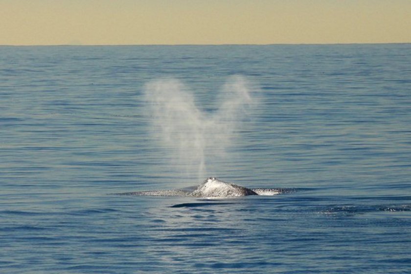
Whale blow, the puff of air mixed with moisture that a whale releases when it comes to the surface, is a famously thrilling indicator of the presence of a whale. From shore, spotting whale blow brings the excitement of knowing that there are whales nearby. During boat-based field work, seeing or hearing blow brings the rush of adrenaline meaning that it’s game time. Whale blow can also be used to identify different species of whales, for example gray whale blow is heart shaped (Figure 1). However, whale blow can be used for more than just spotting and identifying whales. We can use the time between blows to study energetics.
Figure 1. Gray whale blow is often heart shaped (when there is very little wind). Source: https://www.lajollalight.com/sdljl-natural-la-jolla-winter-wildlife-2015jan08-story.html
A blow interval is the time between consecutive blows when a whale is at the surface (Stelle, Megill, and Kinzel 2008). These are also known as short breath holds, whereas long breath holds are times between surfacings (Sumich 1983). Sumich (1983) hypothesized that short breath holds lead to efficient rates of oxygen use. The body uses oxygen to create energy, so “efficient rate of oxygen use” means that longer breath holds do not use much more oxygen and subsequently do not produce more energy. Surfacings, during which short blow intervals occur, are often thought of as recovery periods for whales. Think of it this way, when you sprint, immediately afterwards you typically need to take a break to just breathe and recover.
We hypothesize that we can use blow intervals as a measure of how strenuous an activity is; shorter blow intervals may indicate that an activity is more energetically demanding (Wursig, Wells, and Croll 1986). Let’s go back to the sprinting analogy and compare the energetic demands of walking and running. Imagine I asked you to walk for five minutes, stop and measure the time between each breath, and then run for five minutes and do the same; after running, you would likely breathe more heavily and take more breaths with less time between them. This result indicates that running is more demanding, which we already know because we can do other experiments with humans to study metabolic rate and related metrics. In the case of gray whales, we cannot do experiments in the same way, but we can use the same analogy. Several studies have examined how blow intervals differ between travelling and foraging.
Wursig, Wells, and Croll (1986) measured blow interval, surfacing time, and estimated dive depth and duration of gray whales in Alaska from a boat during the foraging season. They found that blow intervals were shorter during feeding. They also found that the number of blows per surfacing increased with increasing depth. Overall these findings suggest that during the foraging season, feeding is more strenuous than other behaviors and that deeper dives may be more physiologically stressful.
Stelle, Megill, and Kinzel (2008) studied gray whales foraging off of British Columbia, Canada. They found shorter blow intervals during foraging, intermediate blow intervals during searching, and longer blow intervals during travelling. Interestingly, within feeding behaviors, they found a difference between whales feeding on mysids (krill-like animals that swim in the water column) and whales feeding benthically on amphipods. They found that whales feeding on mysids made more frequent but shorter dives with short blow intervals at surface, while whales feeding benthically had longer dives with longer blow intervals. They hypothesized that this difference in surfacing pattern is because mysids might scatter when disturbed, so gray whales surface more often to allow the mysids swarm to reform. These studies inspired me to start investigating these same questions with my drone video data.
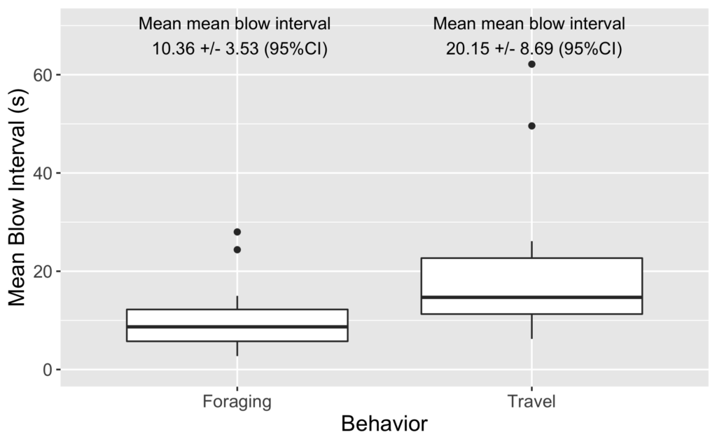
As I review the drone footage and code the behaviors I also mark the time of each blow. I’ve done some initial video coding and using this data I have started to look into differences in blow intervals. As it turns out, we see a similar difference in blow interval relative to behavior state in our data: whales that are foraging have shorter blow intervals than when traveling (Figure 2). It is encouraging to see that our data shows similar patterns.
Figure 2. Boxplot of mean blow interval per sighting of foraging whales and travelling whales.
Next, I would like to examine how blow intervals differ between foraging tactics. A significant part of my thesis is dedicated to studying specific foraging tactics. The perspective from the drone allows us to identify behaviors in greater detail than studies from shore or boat (Torres et al. 2018), allowing us to dig into the differences between the different foraging behaviors. The purpose of foraging is to gain energy. However, this gain is a net gain. To understand the different energetic “values” of each tactic we need to understand the cost of each behavior, i.e. how much energy is required to perform the behavior. Given previous studies, maybe blow intervals could help us measure this cost or at least compare the energetic demands of the behaviors relative to each other. Furthermore, because different behaviors are likely associated with different prey types (Dunham and Duffus 2001), we also need to understand the different energetic gains of each prey type (this is something that Lisa is studying right now, check out the COZI project to learn more). By understanding both of these components – the gains and costs – we can understand the energetic tradeoffs of the different foraging tactics.
Another interesting component to this energetic balance is a whale’s health and body condition. If a whale is in poor health, can it afford the energetic costs of certain behaviors? If whales in poor body condition engage in different behavior patterns than whales in good body condition, are these patterns explained by the energetic costs of the different foraging behaviors? All together this line of investigation is leading to an understanding of why a whale may choose to use different foraging behaviors in different situations. We may never get the full picture; however, I find it really exciting that something as simple and non-invasive as measuring the time between breaths can contribute such a valuable data stream to this project.
References
Dunham, Jason S., and David A. Duffus. 2001. “Foraging Patterns of Gray Whales in Central Clayoquot Sound, British Columbia, Canada.” Marine Ecology Progress Series 223 (November): 299–310. https://doi.org/10.3354/meps223299.
Stelle, Lei Lani, William M. Megill, and Michelle R. Kinzel. 2008. “Activity Budget and Diving Behavior of Gray Whales (Eschrichtius Robustus) in Feeding Grounds off Coastal British Columbia.” Marine Mammal Science 24 (3): 462–78. https://doi.org/10.1111/j.1748-7692.2008.00205.x.
Sumich, James L. 1983. “Swimming Velocities, Breathing Patterns, and Estimated Costs of Locomotion in Migrating Gray Whales, Eschrichtius Robustus.” Canadian Journal of Zoology 61 (3): 647–52. https://doi.org/10.1139/z83-086.
Torres, Leigh G., Sharon L. Nieukirk, Leila Lemos, and Todd E. Chandler. 2018. “Drone up! Quantifying Whale Behavior from a New Perspective Improves Observational Capacity.” Frontiers in Marine Science 5 (SEP). https://doi.org/10.3389/fmars.2018.00319.
Wursig, B., R. S. Wells, and D. A. Croll. 1986. “Behavior of Gray Whales Summering near St. Lawrence Island, Bering Sea.” Canadian Journal of Zoology 64 (3): 611–21. https://doi.org/10.1139/z86-091.
Clara Bird, Masters Student, OSU Department of Fisheries and Wildlife, Geospatial Ecology of Marine Megafauna Lab
Happy new year from the GEMM lab! Starting graduate school comes with a lot of learning. From skills, to learning about how much there is to learn, to learning about the system I will be studying in depth for the next few years. This last category has been the most exciting to me because digging into the literature on a system or a species always leads to the unearthing of some fascinating and surprising facts. So, for this blog I will write about one of the aspects of gray whale foraging that intrigues me most: benthic feeding and its impacts.
How do gray whales
feed?
Gray whales are a unique species. Unlike other baleen whales, such as humpback and blue whales, gray whales regularly feed off the bottom of the ocean (Nerini, 1984). They roll to one side and swim along the bottom, they then suction up (by depressing their tongue) the sediment and prey, then the sediment and water is filtered out of the baleen. In fact, we use sediment streams, shown in Figure 1, as an indicator of benthic feeding behavior when analyzing drone footage (Torres et al. 2018).
Figure 1. Screenshot of drone video showing sediment streaming from mouth of a whale after benthic feeding. Video taken under NOAA/NMFS permit #21678
Locations of benthic feeding can be identified without directly observing a gray whale actively feeding because of the excavated pits that result from benthic feeding (Nerini 1984). These pits can be detected using side-scan sonar that is commonly used to map the seafloor. Oliver and Slattery (1985) found that the pits typically are from 2-20 m2. In some of the imagery, consecutive neighboring pits are visible, likely created by one whale in series during a feeding event. Figure 2 shows different arrangements of pits.
Figure 2. Different arrangements of pits created by feeding whales (Nerini 1984).
Aside from how fascinating the behavior is, benthic feeding is also interesting because it has a large impact on the environment. Coming from a background of studying baleen whales that primarily feed on krill, I had not really considered the potential impacts of whale foraging other than removing prey from the environment. However, when gray whales feed, they excavate large areas of the benthic substrate that disturb and impact the habitat.
The impacts of benthic feeding
Weitkamp et al. (1992) conducted a study on gray whale benthic foraging on ghost shrimp in Puget Sound, WA, USA. This study, conducted over two years, focused on measuring the impact of benthic foraging by its effect on prey abundance. They found that the standing stock of ghost shrimp within a recently excavated pit was two to five times less than that outside the pit, and that 3100 to 5700 grams of shrimp can be removed per pit. From aerial surveys they estimated that within one season feeding gray whales created between 2700 and 3200 pits. Using these values, they calculated that 55 to 79% of the standing stock of ghost shrimp was removed each season by foraging gray whales. Interestingly, they found that the shrimp biomass within an excavated pit recovered within about two months.
Oliver and Slattery (1985) also
found a recovery period of about 2 months per pit in their study on the effect
of gray whale benthic feeding on the prey community in the Bering Sea. They
sampled prey within and outside feeding excavations, both actual whale pits and
man-made, to test the response of the benthic community to the disturbance of a
feeding event. They found that after the initial feeding disturbance, the
excavated area was rapidly colonized by scavenging lysianassid amphipods, which
are small (10 mm) crustaceans that typically eat dead organic material. These
amphipods rushed in and attacked the organisms that were injured or dislodged
by the whale feeding event, typically small crustaceans and polychaete worms.
Within hours of the whale feeding event, these amphipods had dispersed and a
different genre of scavenging lysianassid amphipods slowly invaded the
excavated pit further and stayed much longer. After a few days or weeks these
pits collected and trapped organic debris that attracted more colonists.
Indeed, they found that the number of colonists remained elevated within the
excavated areas for over two months.
Notably, these results on how the
disturbance of gray whale benthic feeding changes sediment composition support
the idea that this foraging behavior maintains the sand substrate and therefore
helps to maintain balanced levels of benthic dwelling amphipods, their primary
source of prey in this study area (Johnson and Nelson, 1984). Gray whales scour
the sea floor when they feed and this process leads to the resuspension of lots
of sediments and nutrients that would otherwise remain on the seafloor.
Therefore, while this feeding may seem like a violent disturbance, it may in
fact play a large role in benthic productivity (Johnson and Nelson, 1984;
Oliver and Slattery, 1985).
These ecosystem impacts of gray
whale benthic feeding I have described above demonstrate the various stages of
invaders after a feeding disturbance, and the process of succession. Succession
is the ecological process of how a community structure builds and grows.
Primary succession is when the structure grows from truly nothing and secondary
succession occurs after a disturbance, such as a fire. In secondary succession,
there are typically pioneer species that first appear and then give way to
other species and a more complex community eventually emerges. Succession is
well documented in many terrestrial studies after disturbance events, and the
processes of secondary succession is very important to community ecology and
resilience.
Since gray whale benthic foraging
does not impact an entire habitat all at once, the process is not perfectly
comparable to secondary succession in terrestrial systems. Yet, when thinking
about the smaller scale, another example of succession in the marine environment
takes place at a whale fall. When a whale dies and sinks to the ocean floor, a
small ecosystem emerges. Different organisms arrive at different stages to
scavenge different parts of the carcass and a food web is created around it.
To
me the impacts of gray whale benthic feeding are akin to both terrestrial disturbance
events and whale falls. The excavation serves as a disturbance, and through secondary
succession the habitat is refreshed via stages of different species colonization
until the system eventually returns to the pre-disturbance levels. However,
like a whale fall the feeding event leaves behind injured or displaced
organisms that scavengers consume; in fact seabirds are known to take advantage
of benthic invertebrates that are brought to the surface by a gray whale feeding
event (Harrison, 1979).
So much of our research is focused
on questions about how the changing environment impacts our study species and
not the other way around. This venture into the literature has provided me with
an important reminder to think about flipping the question. I have enjoyed
starting 2020 with a reminder of how cool gray whales are, and that while a
disturbance can initially be thought of as negative, it may actually bring
about important, and positive, change.
References
Nerini, Mary. 1984. “A Review of Gray Whale Feeding
Ecology.” In The Gray Whale: Eschrichtius Robustus, 423–50. Elsevier
Inc. https://doi.org/10.1016/B978-0-08-092372-7.50024-8.
Oliver, J. S., and P. N. Slattery. 1985. “Destruction and
Opportunity on the Sea Floor: Effects of Gray Whale Feeding.” Ecology 66
(6): 1965–75. https://doi.org/10.2307/2937392.
Torres, Leigh G., Sharon L. Nieukirk, Leila Lemos, and Todd
E. Chandler. 2018. “Drone up! Quantifying Whale Behavior from a New Perspective
Improves Observational Capacity.” Frontiers in Marine Science 5 (SEP).
https://doi.org/10.3389/fmars.2018.00319.
Weitkamp, Laurie A, Robert C Wissmar, Charles A Simenstad,
Kurt L Fresh, and Jay G Odell. 1992. “Gray Whale Foraging on Ghost Shrimp
(Callianassa Californiensis) in Littoral Sand Flats of Puget Sound, USA.” Canadian
Journal of Zoology 70 (11): 2275–80. https://doi.org/10.1139/z92-304.
Johnson, Kirk R., and C. Hans Nelson. 1984. “Side-Scan Sonar
Assessment of Gray Whale Feeding in the Bering Sea.” Science 225 (4667):
1150–52.
Harrison, Craig S. 1979. “The Association of Marine Birds
and Feeding Gray Whales.” The Condor 81 (1): 93.
https://doi.org/10.2307/1367866.
Clara Bird, Masters Student, OSU Department of Fisheries and Wildlife, Geospatial Ecology of Marine Megafauna Lab
The GEMM lab recently completed its fourth field season studying gray whales along the Oregon coast. The 2019 field season was an especially exciting one, we collected rare footage of several interesting gray whale behaviors including GoPro footage of a gray whale feeding on the seafloor, drone footage of a gray whale breaching, and drone footage of surface feeding (check out our recently released highlight video here). For my master’s thesis, I’ll use the drone footage to analyze gray whale behavior and how it varies across space, time, and individual. But before I ask how behavior is related to other variables, I need to understand how to best classify the behaviors.
How do we collect data on behavior?
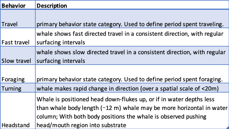
One of the most important tools in behavioral ecology is an ‘ethogram’. An ethogram is a list of defined behaviors that the researcher expects to see based on prior knowledge. It is important because it provides a standardized list of behaviors so the data can be properly analyzed. For example, without an ethogram, someone observing human behavior could say that their subject was walking on one occasion, but then say strolling on a different occasion when they actually meant walking. It is important to pre-determine how behaviors will be recorded so that data classification is consistent throughout the study. Table 1 provides a sample from the ethogram I use to analyze gray whale behavior. The specificity of the behaviors depends on how the data is collected.
Table 1. Sample from gray whale ethogram. Based on ethogram from Torres et al. (2018).
In marine mammal ecology, it is challenging to define specific behaviors because from the traditional viewpoint of a boat, we can only see what the individuals are doing at the surface. The most common method of collecting behavioral data is called a ‘focal follow’. In focal follows an individual, or group, is followed for a set period of time and its behavioral state is recorded at set intervals. For example, a researcher might decide to follow an animal for an hour and record its behavioral state at each minute (Mann 1999). In some studies, they also recorded the location of the whale at each time point. When we use drones our methods are a little different; we collect behavioral data in the form of continuous 15-minute videos of the whale. While we collect data for a shorter amount of time than a typical focal follow, we can analyze the whole video and record what the whale was doing at each second with the added benefit of being able to review the video to ensure accuracy. Additionally, from the drone’s perspective, we can see what the whales are doing below the surface, which can dramatically improve our ability to identify and describe behaviors (Torres et al. 2018).
Categorizing Behaviors
In our ethogram, the behaviors are already categorized into primary states. Primary states are the broadest behavioral states, and in my study, they are foraging, traveling, socializing, and resting. We categorize the specific behaviors we observe in the drone videos into these categories because they are associated with the function of a behavior. While our categorization is based on prior knowledge and critical evaluation, this process can still be somewhat subjective. Quantitative methods provide an objective interpretation of the behaviors that can confirm our broad categorization and provide insight into relationships between categories. These methods include path characterization, cluster analysis, and sequence analysis.
Path characterization classifies behaviors using characteristics of their track line, this method is similar to the RST method that fellow GEMM lab graduate student Lisa Hildebrand described in a recent blog. Mayo and Marx (1990) analyzed the paths of surface foraging North Atlantic Right Whales and were able to classify the paths into primary states; they found that the path of a traveling whale was more linear and then paths of foraging or socializing whales that were more convoluted (Fig 1). I plan to analyze the drone GPS track line as a proxy for the whale’s track line to help distinguish between traveling and foraging in the cases where the 15-minute snapshot does not provide enough context.
Figure 1. Figure from Mayo and Marx (1990) showing different track lines symbolized by behavior category.
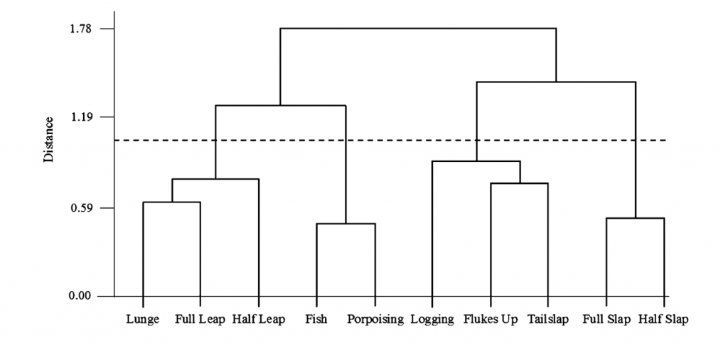
Cluster analysis looks for natural groupings in behavior. For example, Hastie et al. (2004) used cluster analysis to find that there were four natural groupings of bottlenose dolphin surface behaviors (Fig. 2). I am considering using this method to see if there are natural groupings of behaviors within the foraging primary state that might relate to different prey types or habitat. This process is analogous to breaking human foraging down into sub-categories like fishing or farming by looking for different foraging behaviors that typically occur together.
Figure 2. Figure from Hastie et al. (2004) showing the results of a hierarchical cluster analysis.
Lastly, sequence analysis also looks for groupings of behaviors but, unlike cluster analysis, it also uses the order in which behaviors occur. Slooten (1994) used this method to classify Hector’s dolphin surface behaviors and found that there were five classes of behaviors and certain behaviors connected the different categories (Fig. 3). This method is interesting because if there are certain behaviors that are consistently in the same order then that indicates that the order of events is important. What function does a specific sequence of behaviors provide that the behaviors out of that order do not?
Figure 3. Figure from Slooten (1994) showing the results of sequence analysis.
Think about harvesting fruits and
vegetables from a garden: the order of how things are done matters and you
might use different methods to harvest different kinds of produce. Without
knowing what food was being harvested, these methods could detect that there
were different harvesting methods for different fruits or veggies. By then
studying when and where the different methods were used and by whom, we could
gain insight into the different functions and patterns associated with the
different behaviors. We might be able to detect that some methods were always
used in certain habitat types or that different methods were consistently used
at different times of the year.
Behavior classification methods such as these described provide a more refined and detailed analysis of categories that can then be used to identify patterns of gray whale behaviors. While our ultimate goal is to understand how gray whales will be affected by a changing environment, a comprehensive understanding of their current behavior serves as a baseline for that future study.
References
Burnett, J. D., Lemos,
L., Barlow, D., Wing, M. G., Chandler, T., & Torres, L. G. (2019).
Estimating morphometric attributes of baleen whales with photogrammetry from
small UASs: A case study with blue and gray whales. Marine Mammal Science, 35(1),
108–139. https://doi.org/10.1111/mms.12527
Darling, J. D., Keogh, K. E., & Steeves, T. E. (1998).
Gray whale (Eschrichtius robustus) habitat utilization and prey species off
Vancouver Island, B.C. Marine Mammal
Science, 14(4), 692–720.
https://doi.org/10.1111/j.1748-7692.1998.tb00757.x
Hastie, G. D., Wilson, B., Wilson, L. J., Parsons, K. M.,
& Thompson, P. M. (2004). Functional mechanisms underlying cetacean
distribution patterns: Hotspots for bottlenose dolphins are linked to foraging.
Marine Biology, 144(2), 397–403. https://doi.org/10.1007/s00227-003-1195-4
Mann, J. (1999). Behavioral sampling methods for cetaceans:
A review and critique. Marine Mammal
Science, 15(1), 102–122.
https://doi.org/10.1111/j.1748-7692.1999.tb00784.x
Slooten, E. (1994). Behavior of Hector’s Dolphin:
Classifying Behavior by Sequence Analysis. Journal
of Mammalogy, 75(4), 956–964.
https://doi.org/10.2307/1382477
Torres, L. G., Nieukirk, S. L., Lemos, L., & Chandler,
T. E. (2018). Drone up! Quantifying whale behavior from a new perspective
improves observational capacity. Frontiers
in Marine Science, 5(SEP).
https://doi.org/10.3389/fmars.2018.00319
Mayo, C. A., & Marx, M. K. (1990). Surface foraging
behaviour of the North Atlantic right whale, Eubalaena glacialis, and
associated zooplankton characteristics. Canadian
Journal of Zoology, 68(10),
2214–2220. https://doi.org/10.1139/z90-308
By Lisa Hildebrand, MSc student, OSU Department of Fisheries and Wildlife, Geospatial Ecology of Marine Megafauna Lab
For my research in Port Orford, my field team and I track individual gray whales continuously from a shore-based location: once we spot a whale we will track it for the entire time that it remains in our study site. The time spent tracking a whale can vary widely. In the 2018 field season, our shortest trackline was three minutes, and our longest track was over three hours in duration.
This variability in foraging time is partly what sparked my curiosity to investigate potential foraging differences between individuals of the Pacific Coast Feeding Group (PCFG) gray whales. I want to know why some individuals, like “Humpy” who was our longest tracked individual in 2018, stayed in an area for so long, while others, like “Smokey”, only stayed for three minutes (Figure 1). It is hard to pinpoint just one variable that drives these decisions (e.g., prey, habitat) made by individuals about where they forage and how long because the marine environment is so dynamic. Foraging decisions are likely dictated by several factors acting in concert with one another. As a result, I have many research questions, including (but certainly not limited to):
Does prey density drive length of individual foraging bouts?
Do individual whales have preferences for a particular prey species?
Are prey patches containing gravid zooplankton targeted more by whales?
Do whales prefer to feed closer to kelp patches?
How does water depth factor into all of the above decisions and/or preferences?
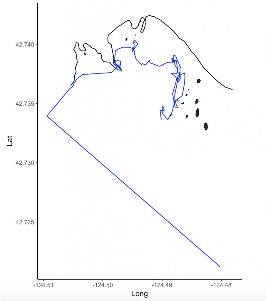
I hope to get to the bottom of these questions through the data analyses I will be undertaking for my second chapter of my Master’s thesis. However, before I can answer those questions, I need to do a little bit of tidying up of my whale tracklines. Now that the 2019 field season is over and I have all of the years of data that I will be analyzing for my thesis (2015-2019), I have spent the past 1-2 weeks diving into the trackline clean-up and analysis preparation.
The first step in this process is to run a speed filter over each trackline. The aim of the speed filter is to remove any erroneous points or outliers that must be wrong based on the known travel speeds of gray whales. Barb Lagerquist, a Marine Mammal Institute (MMI) colleague who has tracked gray whales for several field seasons, found that the fastest individual she ever encountered traveled at a speed of 17.3 km/h (personal communication). Therefore, based on this information, my tracklines are run through a speed filter set to remove any points that suggest that the whale traveled at 17.3 km/h or faster (Figure 2).
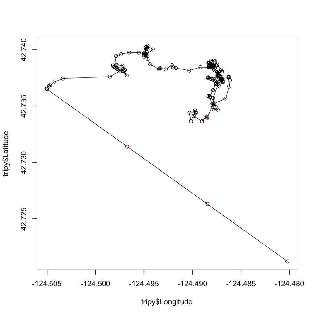
Fig 3. Trackline of “Humpy” after interpolation. The red points are interpolated.
Next, the speed-filtered tracklines are interpolated (Figure 3). Interpolation fills spatial and/or temporal gaps in a data set by evenly spacing points (by distance or time interval) between adjacent points. These gaps sometimes occur in my tracklines when the tracking teams misses one or several surfacings of a whale or because the whale is obscured by a large rock.
After speed filtration and interpolation has occurred, the tracklines are ready to be analyzed using Residence in Space and Time (RST; Torres et al. 2017) to assign behavior state to each location. The questions I am hoping to answer for my thesis are based upon knowing the behavioral state of a whale at a given location and time. In order for me to draw conclusions over whether or not a whale prefers to forage by a reef with kelp rather than a reef without kelp, or whether it prefers Holmesimysis sculpta over Neomysis rayii, I need to know when a whale is actually foraging and when it is not. When we track whales from our cliff site, we assign a behavior to each marked location of an individual. It may sound simple to pick the behavior a whale is currently exhibiting, however it is much harder than it seems. Sometimes the behavioral state of a whale only becomes apparent after tracking it for several minutes. Yet, it’s difficult to change behaviors retroactively while tracking a whale and the qualitative assignment of behavior states is not an objective method. Here is where RST comes in.
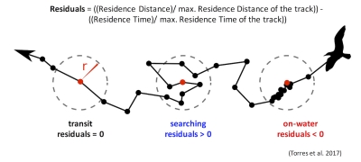
Those of you who have been following the blog for a few years may recall a post written in early 2017 by Rachael Orben, a former post-doc in the GEMM Lab who currently leads the Seabird Oceanography Lab. The post discussed the paper “Classification of Animal Movement Behavior through Residence in Space Time” written by Leigh and Rachael with two other collaborators, which had just been published a few days prior. If you want to know the nitty gritty of what RST is and how it works, I suggest reading Rachael’s blog, the GEMM lab’s brief description of the project and/or the actual paper since it is an open-access publication. However, in a nut shell, RST allows a user to identify three primary behavioral states in a tracking dataset based on the time and distance the individual spent within a given radius. The three behavioral categories are as follows:
Fig 4. Visualization of the three RST behavioral categories. Taken from Torres et al. (2017).
Transit – characterized by short time and distance spent within an area (radius of given size), meaning the individual is traveling.
Time-intensive – characterized by a long time spent within an area, meaning the individual is spending relatively more time but not moving much distance (such as resting in one spot).
Time & distance-intensive – characterized by relatively high time and distances spent within an area, meaning the individual is staying within and moving around a lot in an area, such as searching or foraging.
What behavior these three categories represent depends on the resolution of the data analyzed. Is one point every day for two years? Then the data are unlikely to represent resting. Or is the data 1 point every second for 1 hour? In which case travel segments may cover short distances. On average, my gray whale tracklines are composed of a point every 4-5 minutes for 1-2 hours. Bases on this scale of tracking data, I will interpret the categories as follows: Transit is still travel, time & distance-intensive points represent locations where the whale was searching because it was moving around one area for a while, and time-intensive points represent foraging behavior because the whale has ‘found what it is looking for’ and is spending lots of time there but not moving around much anymore. The great thing about RST is that it removes the bias that is introduced by my field team when assigning behavioral states to individual whales (Figure 5). RST looks at the tracklines in a very objective way and determines the behavioral categories quantitatively, which helps to remove the human subjectivity.
While it took quite a bit of troubleshooting in R and overcoming error messages to make the codes run on my data, I am proud to have results that are interesting and meaningful with which I can now start to answer some of my many research questions. My next steps are to create interpolated prey density and distance to kelp layers in ArcGIS. I will then be able to overlay my cleaned up tracklines to start teasing out potential patterns and relationships between individual whale foraging movements and their environment.
Literature cited
Torres, L. G., R. A. Orben, I. Tolkova, and D. R. Thompson. 2017. Classification of animal movement behavior through residence in space and time. PLoS ONE: doi. org/10.1371/journal.pone.0168513.
By Lisa Hildebrand, MSc student, OSU Department of Fisheries and Wildlife, Geospatial Ecology of Marine Megafauna Lab
It seems unfathomable to me that one year and two months ago I had never used a theodolite before, never been in an ocean kayak before, never identified zooplankton before, never seen a Time-Depth-Recorder (TDR) before. Now, one year later, it seems like all of those tools, techniques and things are just a couple of old friends with which I am being reunited with again. My second field season as the project team lead of the gray whale foraging ecology project in Port Orford (PO) is slowly getting underway and so many of the lessons I learned from my first field season last year have already helped me tremendously this year. I know how to interpret weather forecasts and determine whether it will be a kayak-appropriate day. I know how to figure out the quirks of Pythagoras, the program we use to interface with our theodolite which helps us track whales from our cliff site. I know how to keep track of a budget and feed a team of hungry researchers after a long day of work. Knowing all of these things ahead of this year’s field season have made me feel a little more prepared and at ease with the training of my team and the work to be done. Nevertheless, there are always new curveballs to be thrown my way and while they can often be frustrating, I enjoy the challenges that being a team leader has to offer as it allows me to continue to grow as a field research scientist.
Figure 1. Crew Cinco tracks a whale in Tichenor Cove. Source: L Hildebrand.
2019 marks the fifth year that this project has been taking place in PO. Back in the summer of 2015, former GEMM Lab Master’s student Florence Sullivan started this project together with Leigh. That year the research focused more on investigating vessel disturbance to gray whales by comparing sites of heavy (Boiler Bay) to low boat traffic (Port Orford). The effort found that there were significant differences in gray whale activity budgets between the heavy and low boat traffic conditions (Sullivan & Torres 2018). The following year, the focus of the research switched to being more on the foraging ecology side of things and the project was based solely out of Port Orford, as it continues to be to this day. Being in our fifth year means that we are starting to build a humbly-sized database of sightings across multiple years allowing me to investigate potential individual specialization of the whales that we document. Similarly, multiple years of prey sampling is starting to reveal temporal and spatial trends of prey community assemblages.
Figure 2. Buttons (pictured above) is one of the stars of the Port Orford gray whale foraging ecology project as he has been seen every year since 2016. Crew Cinco has already seen him three times since the start of August. Source: L Hildebrand.
It has become a tradition to come up with a name for the field team that spends 6 weeks at the Oregon State University (OSU) Port Orford Field Station to collect the data for the project. It started with Team Ro“buff”stus in 2015, which I believe carried through until 2017. This is understandable since it’s such a clever name. It’s a play on the species name for gray whales, robustus, but the word “Buff” has been substituted in the center. Buffs are pieces of cloth sewn into a cylindrical shape, often with fun patterns or colors, that can be used as face masks, headbands, and scarves, which come in very handy when your face is exposed to the elements. Doing this project, we can be confronted by wind, sun, fog and sea water all in one day, so Buffs have definitely served the team members very well over the years. Last year, as the project’s torch was passed from Florence to myself, I felt a new team name was apt, and so last year’s team decided our name would be Team Whale Storm. I believe it was because we said we would take the whale world by storm with our insanely good theodolite tracking and kayak sampling skills. With a new year and new team upon us, a new team name was in order. As the title of this blog post indicates, this year the team is called Crew Cinco. The reason behind this name is that we are the fifth team to carry out this field work. Since the gray whales breed in the lagoons of Baja California, Mexico, I like to think that their native language is Spanish. Hence, we have decided that instead of being Crew Five, we are Crew Cinco, as cinco is the Spanish word for five (besides, alliteration makes for a much better team name).
Now that you are up to speed on the history of the PO gray whale project, let me tell you a little about who is part of Crew Cinco and what we have been up to already.
This year’s Marine Studies Initiative OSU undergraduate intern is Mia Arvizu. Mia has just finished her sophomore year at OSU and majors in Environmental Science. Besides being my co-captain this year in the field, Mia is also undertaking an independent research project which focuses on the relationship between sea urchin abundance, kelp health and gray whale foraging. She will tell you all about this project in a few weeks when she takes over the GEMM lab blog. Aside from her interest in ecology and the way science can be used to help local communities in a changing environment, Mia is a dancer, having performed in several dances in OSU’s annual luau this year, and she is currently teaching herself Spanish and Hawaiian.
Both of our high school interns this year are from Astoria. Anthony Howe has just graduated from Astoria High School and will be starting at Clatsop Community College in the fall. His plan is to transfer to OSU and to pursue his interest in marine biology. Anthony, like myself, was born in Germany and lived there until he was six, which means that he is able to speak fluent German. He also introduced the team to the wonders of the Instant Pot, which has made cooking for a team of four hungry scientists much simpler.
Donovan Burns is our other high school intern. He will be going into his junior year in the fall. Donovan never ceases to amaze us with the seemingly endless amounts of general knowledge he has, often sharing facts about Astoria’s history to Asimov’s Laws of Robotics to pickling vegetables, specifically carrots, with us during dinner or while scanning for whales on the cliff site. He also named the first whale we saw here this season – Speckles.
Figure 3. Crew Cinco, from left to right: Anthony Howe, Donovan Burns, Lisa Hildebrand and Mia Arvizu. Source: L Torres.
Crew Cinco has already been in PO for two weeks now. After having a full team meeting with Leigh in Newport and a GEMM lab summer pizza party, we headed south to begin our 6-week field season. It’s hard to believe that the two training weeks are already over. The team worked hard to figure out the subtleties of the theodolite, observe different gray whales and start to understand their dive and foraging patterns, undertake a kayak paddle & safety course, as well as CPR and First Aid training, learn about data processing and management, and how to use a variety of gizmos to aid us in data collection. But it hasn’t all been work. We enjoyed a day in the Californian Redwoods on one of our day’s off and picked blueberries at the Twin Creek Ranch, stocking our freezer with several bags of juicy berries. We have played ‘Sorry!’ perhaps one too many times already (we are in desperate need of some more boardgames if anyone wants to send some our way to the field station!), and enjoyed many walks and runs on beautiful Battle Rock Beach.
Crew Cinco in awe of the Redwoods
Crew Cinco’s blueberry harvest
Crew Cinco after their kayak paddle & safety course South Coast Tours
The next four weeks will not be easy – very early mornings, lots of paddling and squinting into the sun, followed by several hours in the lab processing samples and backing up data. But the next four weeks will also be extremely rewarding – learning lots of new skills that will be valuable beyond this 6-week period, revealing ecological trends and relationships, and ultimately (the true reason for why Mia, Anthony, Donovan and myself are more than happy to put in 6 weeks-worth of hard work), the chance to see whales every day up close and personal. Follow Crew Cinco’s journey over the next few weeks as my interns will be posting to the blog for the next three weeks!
References
Sullivan, F.A., & Torres L.G. Assessment of vessel disturbance to gray whales to inform sustainable ecotourism. Journal of Wildlife Management, 2018. 82: 896-905.
By Dominique Kone, Masters Student in Marine Resource Management
By now, I’m sure you’re aware of recent interests to reintroduce sea otters to Oregon. To inform this effort, my research focuses on predicting suitable sea otter habitat and investigating the potential ecological effects if sea otters are reintroduced in the future. This information will help managers gain a better understanding of the potential for sea otters to reestablish in Oregon, as well as how Oregon’s ecosystems may change via top-down processes. These analyses will address some sources of uncertainties of this effort, but there are still many more questions researchers could address to further guide this process. Here, I note some lingering questions I’ve come across in the course of conducting my research. This is not a complete list of all questions that could or should be investigated, but they represent some of the most interesting questions I have and others have in Oregon.
Credit: Todd Mcleish
The questions, and our associated knowledge on each of these topics:
Is there enough available prey to support a robust sea otter population in Oregon?
Sea otters require approximately 30% of their own body weight in food every day (Costa 1978, Reidman & Estes 1990). With a large appetite, they not only need to spend most of their time foraging, but require a steady supply of prey to survive. For predators, we assume the presence of suitable habitat is a reliable proxy for prey availability (Redfern et al. 2006). Whereby, quality habitat should supply enough prey to sustain predators at higher trophic levels.
In making these habitat predictions for sea otters, we must also recognize the potential limitations of this “habitat equals prey” paradigm, in that there may be parcels of habitat where prey is unavailable or inaccessible. In Oregon, there could be unknown processes unique to our nearshore ecosystems that would support less prey for sea otters. This possibility highlights the importance of not only understanding how much suitable habitat is available for foraging sea otters, but also how much prey is available in these habitats to sustain a viable otter population in the future. Supplementing these habitat predictions with fishery-independent prey surveys is one way to address this question.
Credit: Suzi Eszterhas via Smithsonian Magazine
How will Oregon’s oceanographic seasonality alter or impact habitat suitability?
Sea otters along the California coast exist in an environment with persistent Giant kelp beds, moderate to low wave intensity, and year-round upwelling regimes. These environmental variables and habitat factors create productive ecosystems that provide quality sea otter habitat and a steady supply of prey; thus, supporting high densities of sea otters. This environment contrasts with the Oregon coast, which is characterized by seasonal changes in bull kelp and wave intensity. Summer months have dense kelp beds, calm surf, and strong upwellings. While winter months have little to no kelp, weak upwellings, and intense wave climates. These seasonal variations raise the question as to how these temporal fluctuations in available habitat could impact the number of sea otters able to survive in Oregon.
In Washington – an environment like Oregon – sea otters exhibit seasonal distribution patterns in response to intensifying wave climates. During calm summer months, sea otters primarily forage along the outer coast, but move into more protected areas, such as the Strait of Juan de Fuca, during winter months (Laidre et al. 2009). If sea otters were reintroduced to Oregon, we may very well observe similar seasonal movement patterns (e.g. dispersal into estuaries), but the degree to which this seasonal redistribution and reduction in foraging habitat could impact sea otter reestablishment and recovery is currently unknown.
Credit: Oregon Coast Aquarium
In the event of a reintroduction, do northern or southern sea otters have a greater capacity to adapt to Oregon environments?
In the early 1970’s, Oregon’s first sea otter translocation effort failed (Jameson et al. 1982). Since then, hypotheses on the potential ecological differences between northern and southern sea otters have been proposed as potential factors of the failed effort, potentially due to different abilities to exploit specific prey species. Studies have demonstrated that northern and southern sea otters have slight morphological differences – northern otters having larger skulls and teeth than southern otters (Wilson et al. 1991). This finding has created the hypothesis that the northern otter’s larger skull and teeth allow it to consume prey with denser exoskeletons, and thereby can exploit a greater diversity of prey species. However, there appears to be a lack of evidence to suggest larger skulls and teeth translate to greater bite force. Based on morphology alone, either sub-species could be just as successful in exploiting different prey species.
A different direction to address questions around adaptability is to look at similarities in habitat and oceanographic characteristics. Sea otters exist along a gradient of habitat types (e.g. kelp forests, estuaries, soft-sediment environments) and oceanographic conditions (e.g. warm-temperature to cooler sub-Arctic waters) (Laidre et al. 2009, Lafferty et al. 2014). Yet, we currently don’t know how well or quickly otters can adapt when they expand into new habitats that differ from ones they are familiar with. Sea otters must be efficient foragers and need to acquire skills that allow them to effectively hunt specific prey species (Estes et al. 2003). Hypothetically, if we take sea otters from rocky environments where they’ve developed foraging skills to hunt sea urchins and abalones, and place them in a soft-sediment environment, how quickly would they develop new foraging skills to exploit soft-sediment prey species? Would they adapt quickly enough to meet their daily prey requirements?
Credit: Eric Risberg/Associated Press via The Columbian
In Oregon, specifically, how might climate change impact sea otters, and how might sea otters mediate climate impacts?
Climate change has been shown to directly impact many species via changes in temperature (Chen et al. 2011). Some species have specific thermal tolerances, in which they can only survive within a specified temperature range (i.e. maximum and minimum). Once the temperature moves out of that range, the species can either move with those shifting water masses, behaviorally adapt or perish (Sunday et al. 2012). It’s unclear if and how changing temperatures will impact sea otters, directly. However, sea otters could still be indirectly affected via impacts to their prey. If prey species in sea otter habitat decline due to changing temperatures, this would reduce available food for otters. Ocean acidification (OA) is another climate-induced process that could indirectly impact sea otters. By creating chemical conditions that make it difficult for species to form shells, OA could decrease the availability of some prey species, as well (Gaylord et al. 2011).
Interestingly, these pathways between sea otters and climate change become more complex when we consider the potentially mediating effects from sea otters. Aquatic plants – such as kelp and seagrass – can reduce the impacts of climate change by absorbing and taking carbon out of the water column (Krause-Jensen & Duarte 2016). This carbon sequestration can then decrease acidic conditions from OA and mediate the negative impacts to shell-forming species. When sea otters catalyze a tropic cascade, in which herbivores are reduced and aquatic plants are restored, they could increase rates of carbon sequestration. While sea otters could be an effective tool against climate impacts, it’s not clear how this predator and catalyst will balance each other out. We first need to investigate the potential magnitude – both temporal and spatial – of these two processes to make any predictions about how sea otters and climate change might interact here in Oregon.
Credit: National Wildlife Federation
In Summary
There are several questions I’ve noted here that warrant further investigation and could be a focus for future research as this potential sea otter reintroduction effort progresses. These are by no means every question that should be addressed, but they do represent topics or themes I have come across several times in my own research or in conversations with other researchers and managers. I think it’s also important to recognize that these questions predominantly relate to the natural sciences and reflect my interest as an ecologist. The number of relevant questions that would inform this effort could grow infinitely large if we expand our disciplines to the social sciences, economics, genetics, so on and so forth. Lastly, these questions highlight the important point that there is still a lot we currently don’t know about (1) the ecology and natural behavior of sea otters, and (2) what a future with sea otters in Oregon might look like. As with any new idea, there will always be more questions than concrete answers, but we – here in the GEMM Lab – are working hard to address the most crucial ones first and provide reliable answers and information wherever we can.
References:
Chen, I., Hill, J. K., Ohlemuller, R., Roy, D. B., and C. D. Thomas. 2011. Rapid range shifts of species associated with high levels of climate warming. Science. 333: 1024-1026.
Costa, D. P. 1978. The ecological energetics, water, and electrolyte balance of the California sea otter (Enhydra lutris). Ph.D. dissertation, University of California, Santa Cruz.
Estes, J. A., Riedman, M. L., Staedler, M. M., Tinker, M. T., and B. E. Lyon. 2003. Individual variation in prey selection by sea otters: patterns, causes and implications. Journal of Animal Ecology. 72: 144-155.
Gaylord et al. 2011. Functional impacts of ocean acidification in an ecologically critical foundation species. Journal of Experimental Biology. 214: 2586-2594.
Jameson, R. J., Kenyon, K. W., Johnson, A. M., and H. M. Wight. 1982. History and status of translocated sea otter populations in North America. Wildlife Society Bulletin. 10(2): 100-107.
Krause-Jensen, D., and C. M. Duarte. 2016. Substantial role of macroalgae in marine carbon sequestration. Nature Geoscience. 9: 737-742.
Lafferty, K. D., and M. T. Tinker. 2014. Sea otters are recolonizing southern California in fits and starts. Ecosphere.5(5).
Laidre, K. L., Jameson, R. J., Gurarie, E., Jeffries, S. J., and H. Allen. 2009. Spatial habitat use patterns of sea otters in coastal Washington. Journal of Marine Mammalogy. 90(4): 906-917.
Redfern et al. 2006. Techniques for cetacean-habitat modeling. Marine Ecology Progress Series. 310: 271-295.
Reidman, M. L. and J. A. Estes. 1990. The sea otter (Enhydra lutris): behavior, ecology, and natural history. United States Department of the Interior, Fish and Wildlife Service, Biological Report. 90: 1-126.
Sunday, J. M., Bates, A. E., and N. K. Dulvy. 2012. Thermal tolerance and the global redistribution of animals. Nature: Climate Change. 2: 686-690.
Wilson, D. E., Bogan, M. A., Brownell, R. L., Burdin, A. M., and M. K. Maminov. 1991. Geographic variation in sea otters, Ehydra lutris. Journal of Mammalogy. 72(1): 22-36.
By: Alexa Kownacki, Ph.D. Student, OSU Department of Fisheries and Wildlife, Geospatial Ecology of Marine Megafauna Lab
Data analysis is often about parsing down data into manageable subsets. My project, which spans 34 years and six study sites along the California coast, requires significant data wrangling before full analysis. As part of a data analysis trial, I first refined my dataset to only the San Diego survey location. I chose this dataset for its standardization and large sample size; the bulk of my sightings, over 4,000 of the 6,136, are from the San Diego survey site where the transect methods were highly standardized. In the next step, I selected explanatory variable datasets that covered the sighting data at similar spatial and temporal resolutions. This small endeavor in analyzing my data was the first big leap into understanding what questions are feasible in terms of variable selection and analysis methods. I developed four major hypotheses for this San Diego site.
The study species: common bottlenose dolphin (Tursiops truncatus) seen along the California coastline in 2015. Image source: Alexa Kownacki.
Hypotheses:
H1: I predict that bottlenose dolphin sightings along the San Diego transect throughout the years 1981-2015 exhibit clustered distribution patterns as a result of the patchy distributions of both the species’ preferred habitats, as well as the social nature of bottlenose dolphins.
H2: I predict there would be higher densities of bottlenose dolphin at higher latitudes spanning 1981-2015 due to prey distributions shifting northward and less human activities in the northerly sections of the transect.
H3: I predict that during warm (positive) El Niño Southern Oscillation (ENSO) months, the dolphin sightings in San Diego would be distributed more northerly, predominantly with prey aggregations historically shifting northward into cooler waters, due to (secondarily) increasing sea surface temperatures.
H4: I predict that along the San Diego coastline, bottlenose dolphin sightings are clustered within two kilometers of the six major lagoons, with no specific preference for any lagoon, because the murky, nutrient-rich waters in the estuarine environments are ideal for prey protection and known for their higher densities of schooling fishes.
Data Description:
The common bottlenose dolphin (Tursiops truncatus) sighting data spans 1981-2015 with a few gap years. Sightings cover all months, but not in all years sampled. The same transect in San Diego was surveyed in a small, rigid-hulled inflatable boat with approximately a two-kilometer observation area (one kilometer surveyed 90 degrees to starboard and port of the bow).
I wanted to see if there were changes in dolphin distribution by latitude and, if so, whether those changes had a relationship to ENSO cycles and/or distances to lagoons. For ENSO data, I used the NOAA database that provides positive, neutral, and negative indices (1, 0, and -1, respectively) by each month of each year. I matched these ENSO data to my month-date information of dolphin sighting data. Distance from each lagoon was calculated for each sighting.
Figure 1. Map representing the San Diego transect, represented with a light blue line inside of a one-kilometer buffered “sighting zone” in pale yellow. The dark pink shapes are dolphin sightings from 1981-2015, although some are stacked on each other and cannot be differentiated. The lagoons, ranging in size, are color-coded. The transect line runs from the breakwaters of Mission Bay, CA to Oceanside Harbor, CA.
Results:
H1:True, dolphins are clustered and do not have a uniform distribution across this area. Spatial analysis indicated a less than a 1% likelihood that this clustered pattern could be the result of random chance (Fig. 1, z-score = -127.16, p-value < 0.0001). It is well-known that schooling fishes have a patchy distribution, which could influence the clustered distribution of their dolphin predators. In addition, bottlenose dolphins are highly social and although pods change in composition of individuals, the dolphins do usually transit, feed, and socialize in small groups.
Figure 2. Summary from the Average Nearest Neighbor calculation in ArcMap 10.6 displaying that bottlenose dolphin sightings in San Diego are highly clustered. When the z-score, which corresponds to different colors on the graphic above, is strongly negative (< -2.58), in this case dark blue, it indicates clustering. Because the p-value is very small, in this case, much less than 0.01, these results of clustering are strongly significant.
H2:False, dolphins do not occur at higher densities in the higher latitudes of the San Diego study site. The sightings are more clumped towards the lower latitudes overall (p < 2e-16), possibly due to habitat preference. The sightings are closer to beaches with higher human densities and human-related activities near Mission Bay, CA. It should be noted, that just north of the San Diego transect is the Camp Pendleton Marine Base, which conducts frequent military exercises and could deter animals.
Figure 3. Histogram comparing the latitudes with the frequency of dolphin sightings in San Diego, CA. The x-axis represents the latitudinal difference from the most northern part of the transect to each dolphin sighting. Therefore, a small difference would translate to a sighting being in the northern transect areas whereas large differences would translate to sightings being more southerly. This could be read from left to right as most northern to most southern. The y-axis represents the frequency of which those differences are seen, that is, the number of sightings with that amount of latitudinal difference, or essentially location on the transect line. Therefore, you can see there is a peak in the number of sightings towards the southern part of the transect line.
H3: False, during warm (positive) El Niño Southern Oscillation (ENSO) months, the dolphin sightings in San Diego were more southerly. In colder (negative) ENSO months, the dolphins were more northerly. The differences between sighting latitude and ENSO index was significant (p<0.005). Post-hoc analysis indicates that the north-south distribution of dolphin sightings was different during each ENSO state.
Figure 4. Boxplot visualizing distributions of dolphin sightings latitudinal differences and ENSO index, with -1,0, and 1 representing cold, neutral, and warm years, respectively.
H4:True, dolphins are clustered around particular lagoons. Figure 5 illustrates how dolphin sightings nearest to Lagoon 6 (the San Dieguito Lagoon) are always within 0.03 decimal degrees. Because of how these data are formatted, decimal degrees is the easiest way to measure change in distance (in this case, the difference in latitude). In comparison, dolphins at Lagoon 5 (Los Penasquitos Lagoon) are distributed across distances, with the most sightings further from the lagoon.
Figure 5. Bar plot displaying the different distances from dolphin sighting location to the nearest lagoon in San Diego in decimal degrees. Note: Lagoon 4 is south of the study site and therefore was never the nearest lagoon.
I found a significant difference between distance to nearest lagoon in different ENSO index categories (p < 2.55e-9): there is a significant difference in distance to nearest lagoon between neutral and negative values and positive and neutral years. Therefore, I hypothesize that in neutral ENSO months compared to positive and negative ENSO months, prey distributions are changing. This is one possible hypothesis for the significant difference in lagoon preference based on the monthly ENSO index. Using a violin plot (Fig. 6), it appears that Lagoon 5, Los Penasquitos Lagoon, has the widest variation of sighting distances in all ENSO index conditions. In neutral years, Lagoon 0, the Buena Vista Lagoon has multiple sightings, when in positive and negative years it had either no sightings or a single sighting. The Buena Vista Lagoon is the most northerly lagoon, which may indicate that in neutral ENSO months, dolphin pods are more northerly in their distribution.
Figure 6. Violin plot illustrating the distance from lagoons of dolphin sightings under different ENSO conditions. There are three major groups based on ENSO index: “-1” representing cold years, “0” representing neutral years, and “1” representing warm years. On the x-axis are lagoon IDs and on the y-axis is the distance to the nearest lagoon in decimal degrees. The wider the shapes, the more sightings, therefore Lagoon 6 has many sightings within a very small distance compared to Lagoon 5 where sightings are widely dispersed at greater distances.
Bottlenose dolphins foraging in a small group along the California coast in 2015. Image source: Alexa Kownacki.
Takeaways to science and management:
Bottlenose dolphins have a clustered distribution which seems to be related to ENSO monthly indices, and likely, their social structures. From these data, neutral ENSO months appear to have something different happening compared to positive and negative months, that is impacting the sighting distributions of bottlenose dolphins off the San Diego coastline. More research needs to be conducted to determine what is different about neutral months and how this may impact this dolphin population. On a finer scale, the six lagoons in San Diego appear to have a spatial relationship with dolphin sightings. These lagoons may provide critical habitat for bottlenose dolphins and/or for their preferred prey either by protecting the animals or by providing nutrients. Different lagoons may have different spans of impact, that is, some lagoons may have wider outflows that create larger nutrient plumes.
Other than the Marine Mammal Protection Act and small protected zones, there are no safeguards in place for these dolphins, whose population hovers around 500 individuals. Therefore, specific coastal areas surrounding lagoons that are more vulnerable to habitat loss, habitat degradation, and/or are more frequented by dolphins, may want greater protection added at a local, state, or federal level. For example, the Batiquitos and San Dieguito Lagoons already contain some Marine Conservation Areas with No-Take Zones within their reach. The city of San Diego and the state of California need better ways to assess the coastlines in their jurisdictions and how protecting the marine, estuarine, and terrestrial environments near and encompassing the coastlines impacts the greater ecosystem.
This dive into my data was an excellent lesson in spatial scaling with regards to parsing down my data to a single study site and in matching my existing data sets to other data that could help answer my hypotheses. Originally, I underestimated the robustness of my data. At first, I hesitated when considering reducing the dolphin sighting data to only include San Diego because I was concerned that I would not be able to do the statistical analyses. However, these concerns were unfounded. My results are strongly significant and provide great insight into my questions about my data. Now, I can further apply these preliminary results and explore both finer and broader scale resolutions, such as using the more precise ENSO index values and finding ways to compare offshore bottlenose dolphin sighting distributions.
By Lisa Hildebrand, MSc student, OSU Department of Fisheries and Wildlife, Geospatial Ecology of Marine Megafauna Lab
Every season, or significant period of time, usually has a distinct event that marks its beginning. For example, even though winter officially begins when the winter solstice occurs sometime between December 20 and December 23, many people often associate the first snowfall as the real start of winter. To mark the beginning of schooling, when children start 1stgrade in Germany (which is where I’m from), they receive something called a “Zuckertüte”, which translated means “sugar bag”. It is a large (sometimes as large as the child) cone-shaped container made of cardboard filled with toys, chocolates, sweets, school supplies and various other treats topped with a large bow.
Receiving my Zuckertüte in August of 2001 before starting 1st grade. Source: Ines Hildebrand.
I still remember (and even have) mine – it was almost as tall as I was, had a large Barbie printed on it (and a real one sitting on top of it) and was bright pink. And of course, while at a movie theatre, once the lights dim completely and the curtain surrounding the screen opens just a little further, members of the audience stop chit-chatting or sending text messages, everyone quietens down and puts their devices away – the film is about to start. There are hundreds upon thousands of examples like these – moments, events, days that mark the start of something.
In the past, the beginning of summer has always been tied to two things for me: the end of school and the chance to be outside in the sun for many hours and days. This reality has changed slightly since moving to Oregon. While I don’t technically have any classes during the summer, the work definitely won’t stop. There are still dozens of papers to read, samples to run in the lab, and data points to plot. For anyone from Oregon or the Pacific Northwest (PNW), it’s pretty well known that the weather can be a little unpredictable and variable, meaning that summer might not always be filled with sunny days. Despite somewhat losing these two “summer markers”, I have found a new event to mark the beginning of summer – the arrival of the gray whales.
Their propensity for coastal waters and near-shore feeding is part of what makes gray whales so unique and arguably “easier” to study than some other baleen whale species. Image captured under NOAA/NMFS permit #21678. Source: Leigh Torres.
It’s official – the gray whale field season is upon us! As many of you may already know, the GEMM Lab has two active gray whale research projects: investigating the impacts of ocean noise on gray whale physiology and exploring potential individual foraging specialization among the Pacific Coast Feeding Group (PCFG) gray whales. Both projects involve field work, with the former operating out of Newport and the latter taking place in Port Orford, both collecting photographs and a variety of samples and tracklines to study the PCFG, which is a sub-group of the larger Eastern North Pacific (ENP) population. June 1st is the widely accepted “cut-off date” for the PCFG whales, whereby gray whales seen after June 1st along the PNW coastline (specifically northern California, Oregon, Washington and British Columbia) are considered members of the PCFG. While this date is not the only qualifying factor for an individual to be considered a PCFG member, it is a good general rule of thumb. Since last week happened to be the first week of June, PI Leigh Torres, field technician Todd Chandler and myself launched out onto the Pacific Ocean in our trusty RHIB Ruby twice looking for gray whales, and it sure was a successful start to the season!
Even though I have done small boat-based field work before, every project and field team operates a little differently, which is why I was a little nervous at first. There are a lot of components to the Newport-based project as Leigh & co. assess gray whale physiology by collecting fecal samples, drone imagery and taking photographs, observing behavior patterns, as well as assessing local prey through GoPro footage and light traps. I wasn’t worried about the prey components of the research, since there is plenty of prey sampling involved in my Port Orford research, however I was worried about the whale side of things. I wasn’t sure whether I would be able to catch the drone as it returned back home to Ruby, fearing I might fumble and let it slip through my fingers. I also experienced slight déjà vu when handling the net we use to collect the fecal samples as I was forced to think back to some previous field work that involved collecting a biopsy dart with a net as well. During that project, I had somehow managed to get the end of the net stuck in the back of the boat and as I tried to scoop up the biopsy dart with the net-end, the pole became more and more stuck while the water kept dragging the net-end down and eventually the pole ended up snapping in my hands. On top of all this anxiety and work, trying to find your footing in a small RHIB like Ruby packed with lots of gear and a good amount of swell doesn’t make any of those tasks any easier.
However, as it turned out, none of my fears came to fruition. As soon as Todd fired up Ruby’s engine and we whizzed out and under the Newport bridge, I felt exhilarated. I love field work and was so excited to be out on the water again. During the two days I was able to observe multiple individuals of a species of whale that I find unique and fascinating.
Markings and pigmentation on the flukes are also unique to individuals and allow us to perform photo identification to track individuals over months and years. Image captured under NOAA/NMFS permit #21678. Source: Leigh Torres.
I felt back in my natural element and working with Leigh and Todd was rewarding and fun, as I have so much to learn from their years of experience and natural talent in the field dealing with stressful situations and juggling multiple components and gear. Even though I wasn’t out there collecting data for my own project, some of my observations did get me thinking about what I hope to focus on in my thesis – individualization. It is always interesting to see how differently whales will behave, whether due to the substrate we find them over, the water depths we find them in, or what their surfacing patterns are like. Although I still have six weeks to go until my field season starts and feel lucky to have the opportunity to help Leigh and Todd with the Newport field work, I am already looking forward to getting down to Port Orford in mid-July and starting the fifth consecutive gray whale field season down there.
But back to Newport – over the course of two days, we were able to deploy and retrieve one light trap to collect zooplankton, collect two fecal samples, perform two GoPro drops, fly the drone three times, and take hundreds of photos of whales. Leigh and Todd were both glad to be reunited with an old friend while I felt lucky to be able to meet such a famous lady – Scarback. A whale with a long sighting history not just for the GEMM Lab but for various researchers along the coast that study this population. Scarback is well-known (and easily identified) by the large concave injury on her back that is covered in whale lice, or cyamids. While there are stories about how Scarback’s wound came to be, it is not known for sure how she was injured. However, what researchers do know is that the wound has not stopped this female from reproducing and successfully raising several calves over her lifetime. After hearing her story from Leigh, I wasn’t surprised that both she and Todd were so thrilled to get both a fecal sample and a drone flight from her early in the season. The two days weren’t all rosy; most of day 1 was shrouded in a cloud of mist resulting in a thin but continuous layer of moisture forming on our clothes, while on day 2 we battled with some pretty big swells (up to 6 feet tall) and in typical Oregon coast style we were victims of a sudden downpour for about 10 minutes. We had some excellent sightings and some not-so-excellent sightings. Sightings where we had four whales surrounding our boat at the same time and sightings where we couldn’t re-locate a whale that had popped up right next to us. It happens.
A local celebrity – Scarback. Image captured under NOAA/NMFS permit #21678. Source: Lisa Hildebrand.
An ecstatic Lisa with wild hair standing in the bow pulpit of Ruby camera at the ready. Source: Leigh Torres.
Field work is certainly one of my favorite things in the world. The smell of the salt, the rustling of cereal bar wrappers, the whipping of hair, the perpetual rosy noses and cheeks no matter how many times you apply and re-apply sunscreen, the awkward hilarity of clambering onto the back of the boat where the engine is housed to take a potty break, the whooshing sound of a blow, the sometimes gentle and sometimes aggressive rocking of the boat, the realization that you haven’t had water in four hours only to chug half of your water in a few seconds, the waft of peanut butter and jelly sandwiches, the circular footprint where a whale has just gracefully dipped beneath the surface slipping away from view. I don’t think I will ever tire of any of those things.
As you may have read in previous blog posts, my research focuses on the ecology of blue whales in New Zealand. Through my MS research and years of work by a dedicated team, we were able to document and describe a population of around 700 blue whales that are unique to New Zealand, present year-round, and genetically distinct from all other known populations [1]. While this is a very exciting discovery, documenting this population has also unlocked a myriad of further questions about these whales. Can we predict when and where the whales are most likely to be? How does their distribution change seasonally? How often do they overlap with anthropogenic activity? My PhD research will aim to answer these questions through models of blue whale distribution patterns relative to their environment at multiple spatial and temporal scales.
Because time at sea for vessel-based surveys is cost-limited and difficult to come by, it is in any scientist’s best interest to collect as many concurrent streams of data as possible while in the field. When Dr. Leigh Torres designed our blue whale surveys that were conducted in 2014, 2016, and 2017, she really did a miraculous job of maximizing time on the water. With more data, more questions can be asked. These complimentary datasets have led to the pursuit of many “side projects”. I am lucky enough to work on these questions in parallel with what will form the bulk of my PhD, and collaborate with a number of people in the process. In this blog post, I’ll give you some short teasers of these “side projects”!
Surface lunge feeding as a foraging strategy for New Zealand blue whales
Most of what we know about blue whale foraging behavior comes from studies conducted off the coast of Southern California[2,3] using suction cup accelerometer tags. While these studies in the California Current ecosystem have led to insights and breakthroughs in our understanding of these elusive marine predators and their prey, they have also led us to adopt the paradigm that krill patches are denser at depth, and blue whales are most likely to target these deep prey patches when they feed. We have combined our prey data with blue whale behavioral data observed via a drone to investigate blue whale foraging in New Zealand, with a particular emphasis on surface feeding as a strategy. In our recent analyses, we are finding that in New Zealand, lunge feeding at the surface may be more than just “snacking”. Rather, it may be an energetically efficient strategy that blue whales have evolved in the region with unique implications for conservation.
Figure 1. A blue whale lunges on an aggregation of krill. UAS piloted by Todd Chandler.
Combining multiple data streams for a comprehensive health assessment
In the field, we collected photographs, blubber biopsy samples, fecal samples, and conducted unmanned aerial system (UAS, a.k.a. “drone”) flights over blue whales. The blubber and fecal samples can be analyzed for stress and reproductive hormone levels; UAS imagery allows us to quantify a whale’s body condition[4]; and photographs can be used to evaluate skin condition for abnormalities. By pulling together these multiple data streams, this project aims to establish a baseline understanding of the variability in stress and reproductive hormone levels, body condition, and skin condition for the population. Because our study period spans multiple years, we also have the ability to look at temporal patterns and individual changes over time. From our preliminary results, we have evidence for multiple pregnant females from elevated pregnancy and stress hormones, as well as apparent pregnancy from the body condition analysis. Additionally, a large proportion of the population appear to be affected by blistering and cookie cutter shark bites.
Figure 2. An example aerial drone image of a blue whale that will be used to asses body condition, i.e. how healthy or malnourished the whale is. (Drone piloted by Todd Chandler).
Figure 3. Images of blue whale skin condition, affected by A) blistering and B) cookie cutter shark bites.
Comparing body shape and morphology between species
The GEMM Lab uses UAS to quantitatively study behavior[5] and health of large whales. From various projects in different parts of the world we have now assimilated UAS data on blue, gray, and humpback whales. We will measure these images to investigate differences in body shape and morphology among these species. We plan to explore how form follows function across baleen whales, based on their different life histories, foraging strategies, and ecological roles.
Figure 4 . Aerial images of A) a blue whale in New Zealand’s South Taranaki Bight, B) a gray whale off the coast of Oregon, and C) a humpback whale off the coast of Washington. Drone piloted by Todd Chandler (A and B) and Jason Miranda (C).
So it goes—my dissertation will contain a series of chapters that build on one another to explore blue whale distribution patterns at increasing scales, as well as a growing number of appendices for these “side projects”. Explorations and collaborations like I’ve described here allow me to broaden my perspectives and diversify my analytical skills, as well as work with many excellent teams of scientists. The more data we collect, the more questions we are able to ask. The more questions we ask, the more we seem to uncover that is yet to be understood. So stay tuned for some exciting forthcoming results from all of these analyses, as well as plenty of new questions, waiting to be posed.
References
Barlow DR et al. 2018 Documentation of a New Zealand blue whale population based on multiple lines of evidence. Endanger. Species Res.36, 27–40. (doi:https://doi.org/10.3354/esr00891)
Hazen EL, Friedlaender AS, Goldbogen JA. 2015 Blue whales (Balaenoptera musculus) optimize foraging efficiency by balancing oxygen use and energy gain as a function of prey density. Sci. Adv.1, e1500469–e1500469. (doi:10.1126/sciadv.1500469)
Goldbogen JA, Calambokidis J, Oleson E, Potvin J, Pyenson ND, Schorr G, Shadwick RE. 2011 Mechanics, hydrodynamics and energetics of blue whale lunge feeding: efficiency dependence on krill density. J. Exp. Biol.214, 131–146. (doi:10.1242/jeb.048157)
Burnett JD, Lemos L, Barlow DR, Wing MG, Chandler TE, Torres LG. 2018 Estimating morphometric attributes on baleen whales using small UAS photogrammetry: A case study with blue and gray whales. Mar. Mammal Sci. (doi:10.1111/mms.12527)
Torres LG, Nieukirk SL, Lemos L, Chandler TE. 2018 Drone Up! Quantifying Whale Behavior From a New Perspective Improves Observational Capacity. Front. Mar. Sci.5. (doi:10.3389/fmars.2018.00319)