How we plan to follow whales

Clara Bird, Masters Student, OSU Department of Fisheries and Wildlife, Geospatial Ecology of Marine Megafauna Lab

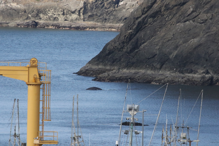
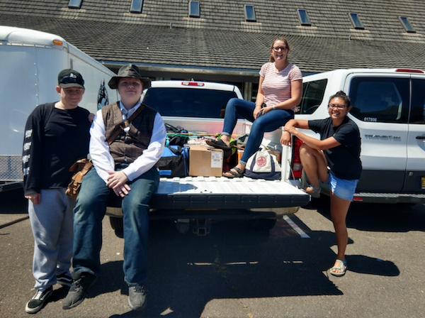
The GEMM Lab gray whale team is in the midst of preparing for our fifth field season studying the Pacific Coast Foraging Group (PCFG): whales that forage off the coast of Newport, OR, USA each summer. On any given good weather day from June to October, our team is out on the water in a small zodiac looking for gray whales (Figure 1). When we find a gray whale, we try to collect photo ID data, fecal samples, drone data, and behavioral data. We use the drone data to study both the whale’s body condition and their behavior. In a previous blog, I described ethograms and how I would like to use the behavior data from drone videos to classify behaviors, with the ultimate goal of understanding how gray whale behavior varies across space, time, and by individual. However, this explanation of studying whale behavior is actually a bit incomplete. Before we start fieldwork, we first need to decide how to collect that data.

Figure 1. Image of GEMM lab team collecting gray whale UAS data. Image taken under NOAA/NMFS permit #16111

As observers, we are far from omnipresent and there is no way to know what the animals are doing all of the time. In any environment, scientists have to decide when and where to observe their animals and what behaviors they are interested in recording. In many studies, behavior is recorded live by an observer. In those studies, other limitations need to be taken into account, such as human error and observer fatigue. Collecting behavioral data is particularly challenging in the marine environment. Cetaceans spend most of their lives out of sight from humans, their time at the surface is brief, and when they appear together in large groups it can be very difficult to keep track of who is doing what when. Imagine being in a boat trying to keep track of what three different whales are doing without a pre-determined method – the task could quickly become overwhelming and biased. This is why we need a methodology for collecting and classifying behavior. We cannot study behavior without acknowledging these limitations and the potential biases that come with the methods we choose. Different data collection methods are better suited to address different questions.

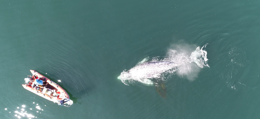
The use of drones gives us the ability to record cetacean behavior non-invasively, from a perspective that allows greater observation (Figure 2, Torres et al. 2018), and for later review, which is a significant improvement. However, as we prepare to collect more behavior data, we need to study the methods and understand the benefits and disadvantages of each approach so that we capture the information we need without bias. Altmann (1974) provides a thorough overview of behavioral sampling methods.

Figure 2. Diagram illustrating “whale surface time” relative to “whale visible time” data as collected from an unmanned aerial systems (UAS) aircraft flying over a gray whale as it moves sequentially (from right to left) from “headstand” foraging to surfacing. Figure from Torres et al. (2018).

Ad libitum behavioral sampling has no structure and occurs when we find a group of whales and just write down everything they are doing. This method is a good first step, however it comes with bias.  Without structure, we cannot be sure that there was an equal probability of detecting each kind of behavior; this problem is called detectability bias. This type of bias is an issue if we are trying to answer questions about how often a behavior occurs, or what percent of time is spent in each behavior state. This is a bias to be especially concerned about when it comes to cetaceans because there are many examples of behaviors with different levels of detectability. An extreme example would be the detectability of breaching versus a behavior that takes place under the surface. A breaching whale is easier to spot and more exciting, which could lead to results suggesting that whales breach more often than they do relative to underwater behaviors. While it’s impossible to eliminate detectability bias, other sampling methods employ decision rules to try and reduce its effect. Many decision rules revolve around time, such as setting a minimum or maximum observation time interval. Other time rules involve recording the behavior state at set intervals of time (e.g., every 5 minutes). Setting observation boundaries helps standardize the methods and the data being collected.

In a structured sampling plan, the first big decision that needs to be addressed is the need to know the duration of behaviors. Point events do not include duration data but can be used to study the frequencies of behaviors. For example, if my research question was “Do whales perform “headstands” in a specific habitat type?”, then I would need point events of headstanding behavior. But, if I wanted to ask, “Do whales spend more time spent headstanding in a specific habitat type than in other habitat types?”, I would need headstanding to be a state event. State events are events with associated duration information and can be used for activity budgets. Activity budgets show how much time an animal spends in each behavior state. Some sampling methods focus on collecting only point events. However, to get the most complete understanding of behavior I think it’s important to collect both. Focal animal follows are another method of collecting more detailed data and is commonly used in cetacean studies.

The explanation of a focal follow method is in the name.  We focus on one individual, follow it, and record all of its behaviors. When employing this method, decisions are made about how an individual is chosen and how long it is followed. In some cases, the behavior of this animal is used as a proxy for the behavior of an entire group. I essentially use the focal follow method in my research. While I review drone footage to record behavioral data instead of recording behaviors live in the field, I focus on one individual a time as I go through the videos. To do this I use a software called BORIS (Friard and Gamba 2016) to mark the time of each behavior per individual (Figure 3). If there are three individuals in a video, I’ll review the footage three times to record behaviors once per individual, focusing on each in turn.

Figure 3. Screenshot of BORIS layout.

While the drone footage brings the advantages of time to review and a better view of the whale, we are constrained by the duration of a flight. Focal follows would ideally last longer than the ~15 minutes of battery life per drone flight. Our previously collected footage gives us snapshots of behavior, and this makes it challenging to compare and analyze durations of behaviors. Therefore, I am excited that we are going to try conducting drone focal follows this summer by swapping out drones when power runs low to achieve longer periods of video coverage of whale behavior. I’ll be able to use these data to move from snapshots to analyzing longer clips and better understanding the behavioral ecology of gray whales. As exciting as this opportunity is, it also presents the challenge of method development. So, I now need to develop decision rules and data collection methods to answer the questions that I have been eagerly asking.

References

Altmann, Jeanne. 1974. “Observational Study of Behavior: Sampling Methods.” Behaviour 49 (3–4): 227–66. https://doi.org/10.1163/156853974X00534.

Friard, Olivier, and Marco Gamba. 2016. “BORIS: A Free, Versatile Open-Source Event-Logging Software for Video/Audio Coding and Live Observations.” Methods in Ecology and Evolution 7 (11): 1325–30. https://doi.org/10.1111/2041-210X.12584.

Torres, Leigh G., Sharon L. Nieukirk, Leila Lemos, and Todd E. Chandler. 2018. “Drone up! Quantifying Whale Behavior from a New Perspective Improves Observational Capacity.” Frontiers in Marine Science 5 (SEP). https://doi.org/10.3389/fmars.2018.00319.

Introducing Crew Cinco – the Port Orford Gray Whale Foraging Ecology Field Team of 2019

By Lisa Hildebrand, MSc student, OSU Department of Fisheries and Wildlife, Geospatial Ecology of Marine Megafauna Lab

It seems unfathomable to me that one year and two months ago I had never used a theodolite before, never been in an ocean kayak before, never identified zooplankton before, never seen a Time-Depth-Recorder (TDR) before. Now, one year later, it seems like all of those tools, techniques and things are just a couple of old friends with which I am being reunited with again. My second field season as the project team lead of the gray whale foraging ecology project in Port Orford (PO) is slowly getting underway and so many of the lessons I learned from my first field season last year have already helped me tremendously this year. I know how to interpret weather forecasts and determine whether it will be a kayak-appropriate day. I know how to figure out the quirks of Pythagoras, the program we use to interface with our theodolite which helps us track whales from our cliff site. I know how to keep track of a budget and feed a team of hungry researchers after a long day of work. Knowing all of these things ahead of this year’s field season have made me feel a little more prepared and at ease with the training of my team and the work to be done. Nevertheless, there are always new curveballs to be thrown my way and while they can often be frustrating, I enjoy the challenges that being a team leader has to offer as it allows me to continue to grow as a field research scientist. 

Figure 1. Crew Cinco tracks a whale in Tichenor Cove. Source: L Hildebrand.

2019 marks the fifth year that this project has been taking place in PO. Back in the summer of 2015, former GEMM Lab Master’s student Florence Sullivan started this project together with Leigh. That year the research focused more on investigating vessel disturbance to gray whales by comparing sites of heavy (Boiler Bay) to low boat traffic (Port Orford). The effort found that there were significant differences in gray whale activity budgets between the heavy and low boat traffic conditions (Sullivan & Torres 2018). The following year, the focus of the research switched to being more on the foraging ecology side of things and the project was based solely out of Port Orford, as it continues to be to this day. Being in our fifth year means that we are starting to build a humbly-sized database of sightings across multiple years allowing me to investigate potential individual specialization of the whales that we document. Similarly, multiple years of prey sampling is starting to reveal temporal and spatial trends of prey community assemblages.

Figure 2. Buttons (pictured above) is one of the stars of the Port Orford gray whale foraging ecology project as he has been seen every year since 2016. Crew Cinco has already seen him three times since the start of August. Source: L Hildebrand.

It has become a tradition to come up with a name for the field team that spends 6 weeks at the Oregon State University (OSU) Port Orford Field Station to collect the data for the project. It started with Team Ro“buff”stus in 2015, which I believe carried through until 2017. This is understandable since it’s such a clever name. It’s a play on the species name for gray whales, robustus, but the word “Buff” has been substituted in the center. Buffs are pieces of cloth sewn into a cylindrical shape, often with fun patterns or colors, that can be used as face masks, headbands, and scarves, which come in very handy when your face is exposed to the elements. Doing this project, we can be confronted by wind, sun, fog and sea water all in one day, so Buffs have definitely served the team members very well over the years. Last year, as the project’s torch was passed from Florence to myself, I felt a new team name was apt, and so last year’s team decided our name would be Team Whale Storm. I believe it was because we said we would take the whale world by storm with our insanely good theodolite tracking and kayak sampling skills. With a new year and new team upon us, a new team name was in order. As the title of this blog post indicates, this year the team is called Crew Cinco. The reason behind this name is that we are the fifth team to carry out this field work. Since the gray whales breed in the lagoons of Baja California, Mexico, I like to think that their native language is Spanish. Hence, we have decided that instead of being Crew Five, we are Crew Cinco, as cinco is the Spanish word for five (besides, alliteration makes for a much better team name).

Now that you are up to speed on the history of the PO gray whale project, let me tell you a little about who is part of Crew Cinco and what we have been up to already.

This year’s Marine Studies Initiative OSU undergraduate intern is Mia Arvizu. Mia has just finished her sophomore year at OSU and majors in Environmental Science. Besides being my co-captain this year in the field, Mia is also undertaking an independent research project which focuses on the relationship between sea urchin abundance, kelp health and gray whale foraging. She will tell you all about this project in a few weeks when she takes over the GEMM lab blog. Aside from her interest in ecology and the way science can be used to help local communities in a changing environment, Mia is a dancer, having performed in several dances in OSU’s annual luau this year, and she is currently teaching herself Spanish and Hawaiian.

Both of our high school interns this year are from Astoria. Anthony Howe has just graduated from Astoria High School and will be starting at Clatsop Community College in the fall. His plan is to transfer to OSU and to pursue his interest in marine biology. Anthony, like myself, was born in Germany and lived there until he was six, which means that he is able to speak fluent German. He also introduced the team to the wonders of the Instant Pot, which has made cooking for a team of four hungry scientists much simpler.

Donovan Burns is our other high school intern. He will be going into his junior year in the fall. Donovan never ceases to amaze us with the seemingly endless amounts of general knowledge he has, often sharing facts about Astoria’s history to Asimov’s Laws of Robotics to pickling vegetables, specifically carrots, with us during dinner or while scanning for whales on the cliff site. He also named the first whale we saw here this season – Speckles. 

Figure 3. Crew Cinco, from left to right: Anthony Howe, Donovan Burns, Lisa Hildebrand and Mia Arvizu. Source: L Torres.

Crew Cinco has already been in PO for two weeks now. After having a full team meeting with Leigh in Newport and a GEMM lab summer pizza party, we headed south to begin our 6-week field season. It’s hard to believe that the two training weeks are already over. The team worked hard to figure out the subtleties of the theodolite, observe different gray whales and start to understand their dive and foraging patterns, undertake a kayak paddle & safety course, as well as CPR and First Aid training, learn about data processing and management, and how to use a variety of gizmos to aid us in data collection. But it hasn’t all been work. We enjoyed a day in the Californian Redwoods on one of our day’s off and picked blueberries at the Twin Creek Ranch, stocking our freezer with several bags of juicy berries. We have played ‘Sorry!’ perhaps one too many times already (we are in desperate need of some more boardgames if anyone wants to send some our way to the field station!), and enjoyed many walks and runs on beautiful Battle Rock Beach. 

The next four weeks will not be easy – very early mornings, lots of paddling and squinting into the sun, followed by several hours in the lab processing samples and backing up data. But the next four weeks will also be extremely rewarding – learning lots of new skills that will be valuable beyond this 6-week period, revealing ecological trends and relationships, and ultimately (the true reason for why Mia, Anthony, Donovan and myself are more than happy to put in 6 weeks-worth of hard work), the chance to see whales every day up close and personal. Follow Crew Cinco’s journey over the next few weeks as my interns will be posting to the blog for the next three weeks!

References

Sullivan, F.A., & Torres L.G. Assessment of vessel disturbance to gray whales to inform sustainable ecotourism. Journal of Wildlife Management, 2018. 82: 896-905. 

Zooming in: A closer look at bottlenose dolphin distribution patterns off of San Diego, CA

By: Alexa Kownacki, Ph.D. Student, OSU Department of Fisheries and Wildlife, Geospatial Ecology of Marine Megafauna Lab

Data analysis is often about parsing down data into manageable subsets. My project, which spans 34 years and six study sites along the California coast, requires significant data wrangling before full analysis. As part of a data analysis trial, I first refined my dataset to only the San Diego survey location. I chose this dataset for its standardization and large sample size; the bulk of my sightings, over 4,000 of the 6,136, are from the San Diego survey site where the transect methods were highly standardized. In the next step, I selected explanatory variable datasets that covered the sighting data at similar spatial and temporal resolutions. This small endeavor in analyzing my data was the first big leap into understanding what questions are feasible in terms of variable selection and analysis methods. I developed four major hypotheses for this San Diego site.

The study species: common bottlenose dolphin (Tursiops truncatus) seen along the California coastline in 2015. Image source: Alexa Kownacki.

Hypotheses:

H1: I predict that bottlenose dolphin sightings along the San Diego transect throughout the years 1981-2015 exhibit clustered distribution patterns as a result of the patchy distributions of both the species’ preferred habitats, as well as the social nature of bottlenose dolphins.

H2: I predict there would be higher densities of bottlenose dolphin at higher latitudes spanning 1981-2015 due to prey distributions shifting northward and less human activities in the northerly sections of the transect.

H3: I predict that during warm (positive) El Niño Southern Oscillation (ENSO) months, the dolphin sightings in San Diego would be distributed more northerly, predominantly with prey aggregations historically shifting northward into cooler waters, due to (secondarily) increasing sea surface temperatures.

H4: I predict that along the San Diego coastline, bottlenose dolphin sightings are clustered within two kilometers of the six major lagoons, with no specific preference for any lagoon, because the murky, nutrient-rich waters in the estuarine environments are ideal for prey protection and known for their higher densities of schooling fishes.

Data Description:

The common bottlenose dolphin (Tursiops truncatus) sighting data spans 1981-2015 with a few gap years. Sightings cover all months, but not in all years sampled. The same transect in San Diego was surveyed in a small, rigid-hulled inflatable boat with approximately a two-kilometer observation area (one kilometer surveyed 90 degrees to starboard and port of the bow).

I wanted to see if there were changes in dolphin distribution by latitude and, if so, whether those changes had a relationship to ENSO cycles and/or distances to lagoons. For ENSO data, I used the NOAA database that provides positive, neutral, and negative indices (1, 0, and -1, respectively) by each month of each year. I matched these ENSO data to my month-date information of dolphin sighting data. Distance from each lagoon was calculated for each sighting.

Figure 1. Map representing the San Diego transect, represented with a light blue line inside of a one-kilometer buffered “sighting zone” in pale yellow. The dark pink shapes are dolphin sightings from 1981-2015, although some are stacked on each other and cannot be differentiated. The lagoons, ranging in size, are color-coded. The transect line runs from the breakwaters of Mission Bay, CA to Oceanside Harbor, CA.

Results: 

H1: True, dolphins are clustered and do not have a uniform distribution across this area. Spatial analysis indicated a less than a 1% likelihood that this clustered pattern could be the result of random chance (Fig. 1, z-score = -127.16, p-value < 0.0001). It is well-known that schooling fishes have a patchy distribution, which could influence the clustered distribution of their dolphin predators. In addition, bottlenose dolphins are highly social and although pods change in composition of individuals, the dolphins do usually transit, feed, and socialize in small groups.

Figure 2. Summary from the Average Nearest Neighbor calculation in ArcMap 10.6 displaying that bottlenose dolphin sightings in San Diego are highly clustered. When the z-score, which corresponds to different colors on the graphic above, is strongly negative (< -2.58), in this case dark blue, it indicates clustering. Because the p-value is very small, in this case, much less than 0.01, these results of clustering are strongly significant.

H2: False, dolphins do not occur at higher densities in the higher latitudes of the San Diego study site. The sightings are more clumped towards the lower latitudes overall (p < 2e-16), possibly due to habitat preference. The sightings are closer to beaches with higher human densities and human-related activities near Mission Bay, CA. It should be noted, that just north of the San Diego transect is the Camp Pendleton Marine Base, which conducts frequent military exercises and could deter animals.

Figure 3. Histogram comparing the latitudes with the frequency of dolphin sightings in San Diego, CA. The x-axis represents the latitudinal difference from the most northern part of the transect to each dolphin sighting. Therefore, a small difference would translate to a sighting being in the northern transect areas whereas large differences would translate to sightings being more southerly. This could be read from left to right as most northern to most southern. The y-axis represents the frequency of which those differences are seen, that is, the number of sightings with that amount of latitudinal difference, or essentially location on the transect line. Therefore, you can see there is a peak in the number of sightings towards the southern part of the transect line.

H3: False, during warm (positive) El Niño Southern Oscillation (ENSO) months, the dolphin sightings in San Diego were more southerly. In colder (negative) ENSO months, the dolphins were more northerly. The differences between sighting latitude and ENSO index was significant (p<0.005). Post-hoc analysis indicates that the north-south distribution of dolphin sightings was different during each ENSO state.

Figure 4. Boxplot visualizing distributions of dolphin sightings latitudinal differences and ENSO index, with -1,0, and 1 representing cold, neutral, and warm years, respectively.

H4: True, dolphins are clustered around particular lagoons. Figure 5 illustrates how dolphin sightings nearest to Lagoon 6 (the San Dieguito Lagoon) are always within 0.03 decimal degrees. Because of how these data are formatted, decimal degrees is the easiest way to measure change in distance (in this case, the difference in latitude). In comparison, dolphins at Lagoon 5 (Los Penasquitos Lagoon) are distributed across distances, with the most sightings further from the lagoon.

Figure 5. Bar plot displaying the different distances from dolphin sighting location to the nearest lagoon in San Diego in decimal degrees. Note: Lagoon 4 is south of the study site and therefore was never the nearest lagoon.

I found a significant difference between distance to nearest lagoon in different ENSO index categories (p < 2.55e-9): there is a significant difference in distance to nearest lagoon between neutral and negative values and positive and neutral years. Therefore, I hypothesize that in neutral ENSO months compared to positive and negative ENSO months, prey distributions are changing. This is one possible hypothesis for the significant difference in lagoon preference based on the monthly ENSO index. Using a violin plot (Fig. 6), it appears that Lagoon 5, Los Penasquitos Lagoon, has the widest variation of sighting distances in all ENSO index conditions. In neutral years, Lagoon 0, the Buena Vista Lagoon has multiple sightings, when in positive and negative years it had either no sightings or a single sighting. The Buena Vista Lagoon is the most northerly lagoon, which may indicate that in neutral ENSO months, dolphin pods are more northerly in their distribution.

Figure 6. Violin plot illustrating the distance from lagoons of dolphin sightings under different ENSO conditions. There are three major groups based on ENSO index: “-1” representing cold years, “0” representing neutral years, and “1” representing warm years. On the x-axis are lagoon IDs and on the y-axis is the distance to the nearest lagoon in decimal degrees. The wider the shapes, the more sightings, therefore Lagoon 6 has many sightings within a very small distance compared to Lagoon 5 where sightings are widely dispersed at greater distances.


Bottlenose dolphins foraging in a small group along the California coast in 2015. Image source: Alexa Kownacki.

Takeaways to science and management: 

Bottlenose dolphins have a clustered distribution which seems to be related to ENSO monthly indices, and likely, their social structures. From these data, neutral ENSO months appear to have something different happening compared to positive and negative months, that is impacting the sighting distributions of bottlenose dolphins off the San Diego coastline. More research needs to be conducted to determine what is different about neutral months and how this may impact this dolphin population. On a finer scale, the six lagoons in San Diego appear to have a spatial relationship with dolphin sightings. These lagoons may provide critical habitat for bottlenose dolphins and/or for their preferred prey either by protecting the animals or by providing nutrients. Different lagoons may have different spans of impact, that is, some lagoons may have wider outflows that create larger nutrient plumes.

Other than the Marine Mammal Protection Act and small protected zones, there are no safeguards in place for these dolphins, whose population hovers around 500 individuals. Therefore, specific coastal areas surrounding lagoons that are more vulnerable to habitat loss, habitat degradation, and/or are more frequented by dolphins, may want greater protection added at a local, state, or federal level. For example, the Batiquitos and San Dieguito Lagoons already contain some Marine Conservation Areas with No-Take Zones within their reach. The city of San Diego and the state of California need better ways to assess the coastlines in their jurisdictions and how protecting the marine, estuarine, and terrestrial environments near and encompassing the coastlines impacts the greater ecosystem.

This dive into my data was an excellent lesson in spatial scaling with regards to parsing down my data to a single study site and in matching my existing data sets to other data that could help answer my hypotheses. Originally, I underestimated the robustness of my data. At first, I hesitated when considering reducing the dolphin sighting data to only include San Diego because I was concerned that I would not be able to do the statistical analyses. However, these concerns were unfounded. My results are strongly significant and provide great insight into my questions about my data. Now, I can further apply these preliminary results and explore both finer and broader scale resolutions, such as using the more precise ENSO index values and finding ways to compare offshore bottlenose dolphin sighting distributions.

Our GEM(M), Ruby, is back in action!

By Lisa Hildebrand, MSc student, OSU Department of Fisheries and Wildlife, Geospatial Ecology of Marine Megafauna Lab

Every season, or significant period of time, usually has a distinct event that marks its beginning. For example, even though winter officially begins when the winter solstice occurs sometime between December 20 and December 23, many people often associate the first snowfall as the real start of winter. To mark the beginning of schooling, when children start 1stgrade in Germany (which is where I’m from), they receive something called a “Zuckertüte”, which translated means “sugar bag”. It is a large (sometimes as large as the child) cone-shaped container made of cardboard filled with toys, chocolates, sweets, school supplies and various other treats topped with a large bow.

Receiving my Zuckertüte in August of 2001 before starting 1st grade. Source: Ines Hildebrand.

I still remember (and even have) mine – it was almost as tall as I was, had a large Barbie printed on it (and a real one sitting on top of it) and was bright pink. And of course, while at a movie theatre, once the lights dim completely and the curtain surrounding the screen opens just a little further, members of the audience stop chit-chatting or sending text messages, everyone quietens down and puts their devices away – the film is about to start. There are hundreds upon thousands of examples like these – moments, events, days that mark the start of something.

In the past, the beginning of summer has always been tied to two things for me: the end of school and the chance to be outside in the sun for many hours and days. This reality has changed slightly since moving to Oregon. While I don’t technically have any classes during the summer, the work definitely won’t stop. There are still dozens of papers to read, samples to run in the lab, and data points to plot. For anyone from Oregon or the Pacific Northwest (PNW), it’s pretty well known that the weather can be a little unpredictable and variable, meaning that summer might not always be filled with sunny days. Despite somewhat losing these two “summer markers”, I have found a new event to mark the beginning of summer – the arrival of the gray whales.

Their propensity for coastal waters and near-shore feeding is part of what makes gray whales so unique and arguably “easier” to study than some other baleen whale species. Image captured under NOAA/NMFS permit #21678. Source: Leigh Torres.


It’s official – the gray whale field season is upon us! As many of you may already know, the GEMM Lab has two active gray whale research projects: investigating the impacts of ocean noise on gray whale physiology and exploring potential individual foraging specialization among the Pacific Coast Feeding Group (PCFG) gray whales. Both projects involve field work, with the former operating out of Newport and the latter taking place in Port Orford, both collecting photographs and a variety of samples and tracklines to study the PCFG, which is a sub-group of the larger Eastern North Pacific (ENP) population. June 1st is the widely accepted “cut-off date” for the PCFG whales, whereby gray whales seen after June 1st along the PNW coastline (specifically northern California, Oregon, Washington and British Columbia) are considered members of the PCFG. While this date is not the only qualifying factor for an individual to be considered a PCFG member, it is a good general rule of thumb. Since last week happened to be the first week of June, PI Leigh Torres, field technician Todd Chandler and myself launched out onto the Pacific Ocean in our trusty RHIB Ruby twice looking for gray whales, and it sure was a successful start to the season!

Even though I have done small boat-based field work before, every project and field team operates a little differently, which is why I was a little nervous at first. There are a lot of components to the Newport-based project as Leigh & co. assess gray whale physiology by collecting fecal samples, drone imagery and taking photographs, observing behavior patterns, as well as assessing local prey through GoPro footage and light traps. I wasn’t worried about the prey components of the research, since there is plenty of prey sampling involved in my Port Orford research, however I was worried about the whale side of things. I wasn’t sure whether I would be able to catch the drone as it returned back home to Ruby, fearing I might fumble and let it slip through my fingers. I also experienced slight déjà vu when handling the net we use to collect the fecal samples as I was forced to think back to some previous field work that involved collecting a biopsy dart with a net as well. During that project, I had somehow managed to get the end of the net stuck in the back of the boat and as I tried to scoop up the biopsy dart with the net-end, the pole became more and more stuck while the water kept dragging the net-end down and eventually the pole ended up snapping in my hands. On top of all this anxiety and work, trying to find your footing in a small RHIB like Ruby packed with lots of gear and a good amount of swell doesn’t make any of those tasks any easier.

However, as it turned out, none of my fears came to fruition. As soon as Todd fired up Ruby’s engine and we whizzed out and under the Newport bridge, I felt exhilarated. I love field work and was so excited to be out on the water again. During the two days I was able to observe multiple individuals of a species of whale that I find unique and fascinating.

Markings and pigmentation on the flukes are also unique to individuals and allow us to perform photo identification to track individuals over months and years. Image captured under NOAA/NMFS permit #21678. Source: Leigh Torres.

I felt back in my natural element and working with Leigh and Todd was rewarding and fun, as I have so much to learn from their years of experience and natural talent in the field dealing with stressful situations and juggling multiple components and gear. Even though I wasn’t out there collecting data for my own project, some of my observations did get me thinking about what I hope to focus on in my thesis – individualization. It is always interesting to see how differently whales will behave, whether due to the substrate we find them over, the water depths we find them in, or what their surfacing patterns are like. Although I still have six weeks to go until my field season starts and feel lucky to have the opportunity to help Leigh and Todd with the Newport field work, I am already looking forward to getting down to Port Orford in mid-July and starting the fifth consecutive gray whale field season down there.

But back to Newport – over the course of two days, we were able to deploy and retrieve one light trap to collect zooplankton, collect two fecal samples, perform two GoPro drops, fly the drone three times, and take hundreds of photos of whales. Leigh and Todd were both glad to be reunited with an old friend while I felt lucky to be able to meet such a famous lady – Scarback. A whale with a long sighting history not just for the GEMM Lab but for various researchers along the coast that study this population. Scarback is well-known (and easily identified) by the large concave injury on her back that is covered in whale lice, or cyamids. While there are stories about how Scarback’s wound came to be, it is not known for sure how she was injured. However, what researchers do know is that the wound has not stopped this female from reproducing and successfully raising several calves over her lifetime. After hearing her story from Leigh, I wasn’t surprised that both she and Todd were so thrilled to get both a fecal sample and a drone flight from her early in the season. The two days weren’t all rosy; most of day 1 was shrouded in a cloud of mist resulting in a thin but continuous layer of moisture forming on our clothes, while on day 2 we battled with some pretty big swells (up to 6 feet tall) and in typical Oregon coast style we were victims of a sudden downpour for about 10 minutes. We had some excellent sightings and some not-so-excellent sightings. Sightings where we had four whales surrounding our boat at the same time and sightings where we couldn’t re-locate a whale that had popped up right next to us. It happens.


A local celebrity – Scarback. Image captured under NOAA/NMFS permit #21678. Source: Lisa Hildebrand.


An ecstatic Lisa with wild hair standing in the bow pulpit of Ruby camera at the ready. Source: Leigh Torres.

Field work is certainly one of my favorite things in the world. The smell of the salt, the rustling of cereal bar wrappers, the whipping of hair, the perpetual rosy noses and cheeks no matter how many times you apply and re-apply sunscreen, the awkward hilarity of clambering onto the back of the boat where the engine is housed to take a potty break, the whooshing sound of a blow, the sometimes gentle and sometimes aggressive rocking of the boat, the realization that you haven’t had water in four hours only to chug half of your water in a few seconds, the waft of peanut butter and jelly sandwiches, the circular footprint where a whale has just gracefully dipped beneath the surface slipping away from view. I don’t think I will ever tire of any of those things.


Marine Mammal Observing: Standardization is key

By: Alexa Kownacki, Ph.D. Student, OSU Department of Fisheries and Wildlife, Geospatial Ecology of Marine Megafauna Lab

For the past two years, I’ve had the opportunity to be the marine mammal observer aboard the NOAA ship Bell M. Shimada for 10 days in May. Both trips covered transects in the Northern California Current Ecosystem during the same time of year, but things looked very different from my chair on the fly bridge. This trip, in particular, highlighted the importance of standardization, seeing as it was the second replicate of the same area. Other scientists and crew members repeatedly asked me the same questions that made me realize just how important it is to have standards in scientific practices and communicating them.

Northern right whale dolphin porpoising out of the water beside the ship while in transit. May 2019. Image source: Alexa Kownacki

The questions:

  1. What do you actually do here and why are you doing it?
  2. Is this year the same as last year in terms of weather, sightings, and transect locations?
  3. Did you expect to see greater or fewer sightings (number and diversity)?
  4. What is this Beaufort Sea State scale that you keep referring to?

All of these are important scientific questions that influence our hypothesis-testing research, survey methods, expected results, and potential conclusions. Although the entire science party aboard the ship conducted marine science, we all had our own specialties and sometimes only knew the basics, if that, about what the other person was doing. It became a perfect opportunity to share our science and standards across similar, but different fields.

Now, to answer those questions:

  1. a) What do you actually do here and b) why are you doing it?

a) As the only marine mammal observer, I stand watch during favorable weather conditions while the ship is in transit, scanning from 0 to 90 degrees off the starboard side (from the front of the ship to a right angle towards the right side when facing forwards). Meanwhile, an application on an iPad called SeaScribe, records the ship’s exact location every 15 seconds, even when no animal is sighted. This process allows for the collection of absence data, that is, data when no animals are present. The SeaScribe program records the survey lines, along with manual inputs that I add, including weather and observer information. When I spot a marine mammal, I immediately mark an exact location on a hand held GPS, use my binoculars to identify the species, and add information to the sighting on the SeaScribe program, such as species, distance to the sighted animal(s), the degree (angle) to the sighting, number of animals in a group, behavior, and direction if traveling.

b) Marine mammal observing serves many different purposes. In this case, observing collects information about what species are where at what time. By piggy-backing on these large-scale, offshore oceanographic NOAA surveys, we have the unique opportunity to survey along standardized transect lines during different times of the year. From replicate survey data, we can start to form an idea of which species use which areas and what oceanographic conditions may impact species distributions. Currently there is not much consistent marine mammal data collected over these offshore areas between Northern California and Washington State, so our work is aiming to fill this knowledge gap.

Alexa observing on the R/V Shimada in May 2019, all bundled up. Image Source: Alexa Kownacki

  1. What is this Beaufort Sea State scale that you keep referring to?

Great question! It took me a while to realize that this standard measuring tool to estimate wind speeds and sea conditions, is not commonly recognized even among other sea-goers. The Beaufort Sea State, or BSS, uses an empirical scale that ranges from 0-12 with 0 being no wind and calm seas, to 12 being hurricane-force winds with 45+ ft seas. It is frequently referenced by scientists in oceanography, marine science, and climate science as a universally-understood metric. The BSS was created in 1805 by Francis Beaufort, a hydrographer in the Royal Navy, to standardize weather conditions across the fleet of vessels. By the mid-1850s, the BSS was standardized to non-naval use for sailing vessels, and in 1916, expanded to include information specific to the seas and not the sails1. We in the marine mammal observation field constantly collect BSS information while on survey to measure the quality of survey conditions that may impact our observations. BSS data allows us to measure the extent of our survey range, both in the distance that we are likely to sight animals and also the likelihood of sighting anything. Therefore, the BSS scale gives us an important indication of how much absence data we have collected, in addition to presence data.

A description of the Beaufort Sea State Scale. Image source: National Weather Service.


  1. Is this year the same as last year in terms of weather, sightings, and transect locations?

The short answer is no. Observed differences in marine mammal sightings in terms of both species diversity and number of animals between years can be normal. There are many potential explanatory variables, from differences in currents, upwelling strength, El Nino index levels, water temperatures, or, what was obvious in this case: sighting conditions. The weather in May 2019 varied greatly from that in May 2018. Last year, I observed for nearly every day because the Beaufort Sea State (BSS) was frequently less than a four. However, this year, more often than not, the BSS greater than or equal to five. A BSS of 5 equates to approximately 17-21 knots of breeze with 6-foot waves and the water appears to have many “white horses” or pronounced white caps with sea spray. Additionally, mechanical issue with winches delayed and altered our transect locations. Therefore, although multiple transects from May 2018 were also surveyed during May 2019, there were a few lines that do not have data for both cruises.

May 2018 with a BSS 1

May 2019 with a BSS 6


  1. Did you expect to see greater or fewer sightings (number and diversity)?

Knowing that I had less favorable sighting conditions and less amount of effort observing this year, it is not surprising that I observed fewer marine mammals in total count and in species diversity. Even less surprising is that on the day with the best weather, where the BSS was less than a five, I recorded the most sightings with the highest species count. May 2018 felt a bit like a tropical vacation because we had surprisingly sunny days with mild winds, and during May 2019 we had some rough seas with gale force winds. Additionally, as an observer, I need to remove as much bias as possible. So, yes, I had hoped to see beaked whales or orca like I did in May 2018, but I was still pleasantly surprised when I spotted fin whales feeding in May 2019.

Marine Mammal Species Number of Sightings
May 2018 May 2019
Humpback whale 31 6
Northern right whale dolphin 1 2
Pacific white-sided dolphin 3 6
UNID beaked whale 1 0
Cuvier’s beaked whale 1 0
Gray whale 4 1
Minke whale 1 1
Fin whale 4 1
Blue whale 1 0
Transient killer whale 1 0
Dall’s porpoise 2 0
Northern fur seal 1 0
California sea lion 0 1

Pacific white-sided dolphin. Image source: Alexa Kownacki

Standardization is a common theme. Observing between years on standard transects, at set speeds, in different conditions using standardized tools is critical to collecting high quality data that is comparable across different periods. Scientists constantly think about quality control. We look for trends and patterns, similarities and differences, but none of those could be understood without having standard metrics.

The entire science party aboard the R/V Shimada in May 2019, including a marine mammal scientist, phytoplankton scientists, zooplankton scientists, and fisheries scientists, and oceanographers. Image Source: Alexa Kownacki

Literature Cited:

1Oliver, John E. (2005). Encyclopedia of world climatology. Springer.


More data, more questions, more projects: There’s always more to learn

By Dawn Barlow, PhD student, OSU Department of Fisheries and Wildlife, Geospatial Ecology of Marine Megafauna Lab 

As you may have read in previous blog posts, my research focuses on the ecology of blue whales in New Zealand. Through my MS research and years of work by a dedicated team, we were able to document and describe a population of around 700 blue whales that are unique to New Zealand, present year-round, and genetically distinct from all other known populations [1]. While this is a very exciting discovery, documenting this population has also unlocked a myriad of further questions about these whales. Can we predict when and where the whales are most likely to be? How does their distribution change seasonally? How often do they overlap with anthropogenic activity? My PhD research will aim to answer these questions through models of blue whale distribution patterns relative to their environment at multiple spatial and temporal scales.

Because time at sea for vessel-based surveys is cost-limited and difficult to come by, it is in any scientist’s best interest to collect as many concurrent streams of data as possible while in the field. When Dr. Leigh Torres designed our blue whale surveys that were conducted in 2014, 2016, and 2017, she really did a miraculous job of maximizing time on the water. With more data, more questions can be asked. These complimentary datasets have led to the pursuit of many “side projects”. I am lucky enough to work on these questions in parallel with what will form the bulk of my PhD, and collaborate with a number of people in the process. In this blog post, I’ll give you some short teasers of these “side projects”!

Surface lunge feeding as a foraging strategy for New Zealand blue whales

Most of what we know about blue whale foraging behavior comes from studies conducted off the coast of Southern California[2,3] using suction cup accelerometer tags. While these studies in the California Current ecosystem have led to insights and breakthroughs in our understanding of these elusive marine predators and their prey, they have also led us to adopt the paradigm that krill patches are denser at depth, and blue whales are most likely to target these deep prey patches when they feed. We have combined our prey data with blue whale behavioral data observed via a drone to investigate blue whale foraging in New Zealand, with a particular emphasis on surface feeding as a strategy. In our recent analyses, we are finding that in New Zealand, lunge feeding at the surface may be more than just “snacking”. Rather, it may be an energetically efficient strategy that blue whales have evolved in the region with unique implications for conservation.

Figure 1. A blue whale lunges on an aggregation of krill. UAS piloted by Todd Chandler.

Combining multiple data streams for a comprehensive health assessment

In the field, we collected photographs, blubber biopsy samples, fecal samples, and conducted unmanned aerial system (UAS, a.k.a. “drone”) flights over blue whales. The blubber and fecal samples can be analyzed for stress and reproductive hormone levels; UAS imagery allows us to quantify a whale’s body condition[4]; and photographs can be used to evaluate skin condition for abnormalities. By pulling together these multiple data streams, this project aims to establish a baseline understanding of the variability in stress and reproductive hormone levels, body condition, and skin condition for the population. Because our study period spans multiple years, we also have the ability to look at temporal patterns and individual changes over time. From our preliminary results, we have evidence for multiple pregnant females from elevated pregnancy and stress hormones, as well as apparent pregnancy from the body condition analysis. Additionally, a large proportion of the population appear to be affected by blistering and cookie cutter shark bites.

Figure 2. An example aerial drone image of a blue whale that will be used to asses body condition, i.e. how healthy or malnourished the whale is. (Drone piloted by Todd Chandler).

Figure 3. Images of blue whale skin condition, affected by A) blistering and B) cookie cutter shark bites.

Comparing body shape and morphology between species

The GEMM Lab uses UAS to quantitatively study behavior[5] and health of large whales. From various projects in different parts of the world we have now assimilated UAS data on blue, gray, and humpback whales. We will measure these images to investigate differences in body shape and morphology among these species. We plan to explore how form follows function across baleen whales, based on their different  life histories, foraging strategies, and ecological roles.

Figure 4 . Aerial images of A) a blue whale in New Zealand’s South Taranaki Bight, B) a gray whale off the coast of Oregon, and C) a humpback whale off the coast of Washington. Drone piloted by Todd Chandler (A and B) and Jason Miranda (C). 

So it goes—my dissertation will contain a series of chapters that build on one another to explore blue whale distribution patterns at increasing scales, as well as a growing number of appendices for these “side projects”. Explorations and collaborations like I’ve described here allow me to broaden my perspectives and diversify my analytical skills, as well as work with many excellent teams of scientists. The more data we collect, the more questions we are able to ask. The more questions we ask, the more we seem to uncover that is yet to be understood. So stay tuned for some exciting forthcoming results from all of these analyses, as well as plenty of new questions, waiting to be posed.

References

  1. Barlow DR et al. 2018 Documentation of a New Zealand blue whale population based on multiple lines of evidence. Endanger. Species Res. 36, 27–40. (doi:https://doi.org/10.3354/esr00891)
  2. Hazen EL, Friedlaender AS, Goldbogen JA. 2015 Blue whales (Balaenoptera musculus) optimize foraging efficiency by balancing oxygen use and energy gain as a function of prey density. Sci. Adv. 1, e1500469–e1500469. (doi:10.1126/sciadv.1500469)
  3. Goldbogen JA, Calambokidis J, Oleson E, Potvin J, Pyenson ND, Schorr G, Shadwick RE. 2011 Mechanics, hydrodynamics and energetics of blue whale lunge feeding: efficiency dependence on krill density. J. Exp. Biol. 214, 131–146. (doi:10.1242/jeb.048157)
  4. Burnett JD, Lemos L, Barlow DR, Wing MG, Chandler TE, Torres LG. 2018 Estimating morphometric attributes on baleen whales using small UAS photogrammetry: A case study with blue and gray whales. Mar. Mammal Sci. (doi:10.1111/mms.12527)
  5. Torres LG, Nieukirk SL, Lemos L, Chandler TE. 2018 Drone Up! Quantifying Whale Behavior From a New Perspective Improves Observational Capacity. Front. Mar. Sci. 5. (doi:10.3389/fmars.2018.00319)

Science (or the lack thereof) in the Midst of a Government Shutdown

By Alexa Kownacki, Ph.D. Student, OSU Department of Fisheries and Wildlife, Geospatial Ecology of Marine Megafauna Lab

In what is the longest government shutdown in the history of the United States, many people are impacted. Speaking from a scientist’s point of view, I acknowledge the scientific community is one of many groups that is being majorly obstructed. Here at the GEMM Laboratory, all of us are feeling the frustrations of the federal government grinding to a halt in different ways. Although our research spans great distances—from Dawn’s work on New Zealand blue whales that utilizes environmental data managed by our federal government, to new projects that cannot get federal permit approvals to state data collection, to many of Leigh’s projects on the Oregon coast of the USA that are funded and collaborate with federal agencies—we all recognize that our science is affected by the shutdown. My research on common bottlenose dolphins is no exception; my academic funding is through the US Department of Defense, my collaborators are NOAA employees who contribute NOAA data; I use publicly-available data for additional variables that are government-maintained; and I am part of a federally-funded public university. Ironically, my previous blog post about the intersection of science and politics seems to have become even more relevant in the past few weeks.

Many graduate students like me are feeling the crunch as federal agencies close their doors and operations. Most people have seen the headlines that allude to such funding-related issues. However, it’s important to understand what the funding in question is actually doing. Whether we see it or not, the daily operations of the United States Federal government helps science progress on a multitude of levels.

Federal research in the United States is critical. Most governmental branches support research with the most well-known agencies for doing so being the National Science Foundation (NSF), the US Department of Agriculture (USDA), the National Oceanic and Atmospheric Administration (NOAA), and the National Aeronautics and Space Administration. There are 137 executive agencies in the USA (cei.org). On a finer scale, NSF alone receives approximately 40,000 scientific proposals each year (nsf.gov).

If I play a word association game and I am given the word “science”, my response would be “data”. Data—even absence data—informs science. The largest aggregate of metadata with open resources lives in the centralized website, data.gov, which is maintained by the federal government and is no longer accessible and directs you to this message:Here are a few more examples of science that has stopped in its track from lesser-known research entities operated by the federal government:

Currently, the National Weather Service (NWS) is unable to maintain or improve its advanced weather models. Therefore, in addition to those of us who include weather or climate aspects into our research, forecasters are having less and less information on which to base their weather predictions. Prior to the shutdown, scientists were changing the data format of the Global Forecast System (GFS)—the most advanced mathematical, computer-based weather modeling prediction system in the USA. Unfortunately, the GFS currently does not recognize much of the input data it is receiving. A model is only as good as its input data (as I am sure Dawn can tell you), and currently that means the GFS is very limited. Many NWS models are upgraded January-June to prepare for storm season later in the year. Therefore, there are long-term ramifications for the lack of weather research advancement in terms of global health and safety. (https://www.washingtonpost.com/weather/2019/01/07/national-weather-service-is-open-your-forecast-is-worse-because-shutdown/?noredirect=on&utm_term=.5d4c4c3c1f59)

An example of one output from the GFS model. (Source: weather.gov)

The Food and Drug Administration (FDA)—a federal agency of the Department of Health and Human Services—that is responsible for food safety, has reduced inspections. Because domestic meat and poultry are at the highest risk of contamination, their inspections continue, but by staff who are going without pay, according to the agency’s commissioner, Dr. Scott Gottlieb. Produce, dry foods, and other lower-risk consumables are being minimally-inspected, if at all.  Active research projects investigating food-borne illness that receive federal funding are at a standstill.  Is your stomach doing flips yet? (https://www.nytimes.com/2019/01/09/health/shutdown-fda-food-inspections.html?rref=collection%2Ftimestopic%2FFood%20and%20Drug%20Administration&action=click&contentCollection=timestopics&region=stream&module=stream_unit&version=latest&contentPlacement=2&pgtype=collection)

An FDA field inspector examines imported gingko nuts–a process that is likely not happening during the shutdown. (Source: FDA.gov)

The National Parks Service (NPS) recently made headlines with the post-shutdown acts of vandalism in the iconic Joshua Tree National Park. What you might not know is that the shutdown has also stopped a 40-year study that monitors how streams are recovering from acid rain. Scientists are barred from entering the park and conducting sampling efforts in remote streams of Shenandoah National Park, Virginia. (http://www.sciencemag.org/news/2019/01/us-government-shutdown-starts-take-bite-out-science)

A map of the sampling sites that have been monitored since the 1980s for the Shenandoah Watershed Study and Virginia Trout Stream Sensitivity Study that cannot be accessed because of the shutdown. (Source: swas.evsc.virginia.edu)

NASA’s Stratospheric Observatory for Infrared Astronomy (SOFIA), better known as the “flying telescope” has halted operations, which will require over a week to bring back online upon funding restoration. SOFIA usually soars into the stratosphere as a tool to study the solar system and collect data that ground-based telescopes cannot. (http://theconversation.com/science-gets-shut-down-right-along-with-the-federal-government-109690)

NASA’s Stratospheric Observatory for Infrared Astronomy (SOFIA) flies over the snowy Sierra Nevada mountains while the telescope gathers information. (Source: NASA/ Jim Ross).

It is important to remember that science happens outside of laboratories and field sites; it happens at meetings and conferences where collaborations with other great minds brainstorm and discover the best solutions to challenging questions. The shutdown has stopped most federal travel. The annual American Meteorological Society Meeting and American Astronomical Society meeting were two of the scientific conferences in the USA that attract federal employees and took place during the shutdown. Conferences like these are crucial opportunities with lasting impacts on science. Think of all the impressive science that could have sparked at those meetings. Instead, many sessions were cancelled, and most major agencies had zero representation (https://spacenews.com/ams-2019-overview/). Topics like lidar data applications—which are used in geospatial research, such as what the GEMM Laboratory uses in some its projects, could not be discussed. The cascade effects of the shutdown prove that science is interconnected and without advancement, everyone’s research suffers.

It should be noted, that early-career scientists are thought to be the most negatively impacted by this shutdown because of financial instability and job security—as well as casting a dark cloud on their futures in science: largely unknown if they can support themselves, their families, and their research. (https://eos.org/articles/federal-government-shutdown-stings-scientists-and-science). Graduate students, young professors, and new professionals are all in feeling the pressure. Our lives are based on our research. When the funds that cover our basic research requirements and human needs do not come through as promised, we naturally become stressed.

An adult and a juvenile common bottlenose dolphin, forage along the San Diego coastline in November 2018. (Source: Alexa Kownacki)

So, yes, funding—or the lack thereof—is hurting many of us. Federally-funded individuals are selling possessions to pay for rent, research projects are at a standstill, and people are at greater health and safety risks. But, also, science, with the hope for bettering the world and answering questions and using higher thinking, is going backwards. Every day without progress puts us two days behind. At first glance, you may not think that my research on bottlenose dolphins is imperative to you or that the implications of the shutdown on this project are important. But, consider this: my study aims to quantify contaminants in common bottlenose dolphins that either live in nearshore or offshore waters. Furthermore, I study the short-term and long-term impacts of contaminants and other health markers on dolphin hormone levels. The nearshore common bottlenose dolphin stocks inhabit the highly-populated coastlines that many of us utilize for fishing and recreation. Dolphins are mammals, that respond to stress and environmental hazards, in similar ways to humans. So, those blubber hormone levels and contamination results, might be more connected to your health and livelihood than at first glance. The fact that I cannot download data from ERDDAP, reach my collaborators, or even access my data (that starts in the early 1980s), does impact you. Nearly everyone’s research is connected to each other’s at some level, and that, in turn has lasting impacts on all people—scientists or not. As the shutdown persists, I continue to question how to work through these research hurdles. If anything, it has been a learning experience that I hope will end soon for many reasons—one being: for science.

GEMM Lab 2018: A Year in the Life

By Dawn Barlow, PhD student, Department of Fisheries & Wildlife, Geospatial Ecology of Marine Megafauna Lab

As 2018 draws to a close, it is gratifying to step back and appreciate the accomplishments of the past year. For all members of the GEMM Lab, 2018 has certainly been one for the books! Here are some of our highlights for your holiday enjoyment.

We conducted fieldwork to collect new data in multiple seasons, multiple hemispheres, and across oceans. For the first time, GEMM Lab members joined the Northern California Current Ecosystem cruises aboard NOAA ship Bell M. Shimada as marine mammal observers—Florence in February, Alexa in May, and me in September.

Summertime in the Pacific Northwest brings the gray whales to the Oregon Coast. The drone-flying, poop-scooping, plankton-trapping team of Leigh, Todd, Leila, Joe, and Sharon took to the water for the third year to investigate the health of this gray whale population. It was a successful field season, ending with 72 fecal samples collected! Visiting students joined our experienced members to shadow the gray whale fieldwork—Julia Stepanuk and Alejandro Fernandez Ajo came from across the country to hop on board with us for a bit. Friendship and collaboration were built quickly in a little boat chasing after whale poop, bonding over peanut butter and jelly sandwiches.

Another GEMM Lab team tracked the gray whales from the cliff in Port Orford. Lisa Hildebrand joined us as the GEMM Lab’s newest graduate student, and immediately led a team of interns on Oregon’s southern coast to track gray whale movements and sample their prey from a trusty research kayak.

The summer 2018 gray whale foraging ecology team, affectionately known as “team whale storm”, at the Port Orford Field Station.

Rachael observed seabirds from Yaquina Head in May and June, where the colony of common murres had the highest reproductive success in 10 years! Then she left the summertime in July to travel to the other end of the world, braving winter in the remote South Atlantic to study South American fur seals in the Falkland Islands.

Dr. Rachael Orben and Dr. Alistair Bayliss looking out towards the fur seals. Photo: Kayleigh Jones

In New Caledonia, Solene and a research team ventured to Antigonia Seamount and Orne Bank to study the use of these offshore areas by breeding humpback whales. They collected numerous biopsy samples and successfully deployed satellite tags. Solene was also selected to receive the Louis Herman research scholarship to continue studying humpback whale movement and diving behavior around seamounts.

Sorting biopsy samples during a successful expedition to study humpback whales around remote seamounts in the South Pacific.

Beyond fieldwork, our members have been busily disseminating our findings. In July, Leigh and I traveled to Wellington to present our latest findings on New Zealand blue whales to scientists, managers, politicians, industry representatives, and advocacy groups. Because of our documentation of a unique New Zealand blue whale population, which was published earlier this year, the New Zealand government has proposed to create a Marine Mammal Sanctuary for the protection of blue whales. This is quite a feat, considering blue whales were classified as only “migrant” in New Zealand waters prior to our work. Fueled by flat whites in wintery Wellington, we navigated government buildings, discussing blue whale distribution patterns, overlap with the oil and gas industry, what we now know based on our latest analyses, and what we consider to be the most pressing gaps in our knowledge.

Dr. Leigh Torres and Dawn Barlow in front of Parliament in Wellington, New Zealand following the presentation of their recent findings.

Alexa spent the summer and fall in San Diego, where she collaborated with researchers at NOAA Southwest Fisheries Science Center on her study of about the health of bottlenose dolphins off the California coast. Her time down south has been productive and we look forward to having her back in Oregon with us to round out the second year of her PhD program.

In the fall, Dom and Leigh participated in the first ever Oregon Sea Otter Status of Knowledge Symposium. With growing interest in a potential sea otter reintroduction, the symposium brought together a range of experts – including scientists, managers, and tribes – to discuss what we currently know about sea otters in other regions and how this knowledge could be applied to an Oregon reintroduction effort. Dom was one of many speakers at this event, and gave a well-received talk on Oregon’s previous sea otter reintroduction attempt and brief discussion on his thesis research. Over the next year, Dom not only plans to finish his thesis, but also to join an interdisciplinary research team to further investigate other social, genetic, and ecological implications of a potential sea otter reintroduction.

Sea otter mom and pup. Source: Hakai Magazine.

2018-19 OSU NRT Cohort. Source: Oregon State University.

Several GEMM Lab members reached academic milestones this year. Rachael was promoted to Assistant Professor in the spring! She now leads the Seabird Oceanography Lab, and remains involved in multiple projects studying seabirds and pinnipeds all over the world. Leila passed her PhD qualifying exams and advanced to candidacy in the spring, a major accomplishment toward completing her doctoral degree. I successfully defended my MS degree in June, and my photo was added to our wall gallery of GEMM Lab graduates. I won’t be leaving the GEMM Lab anytime soon, however, as I will be continuing my research on New Zealand blue whales as a PhD student. The GEMM Lab welcomed a new MS student in the summer—Lisa Hildebrand will be studying gray whale foraging ecology on the Oregon Coast. Welcome, Lisa! In early December, Solene successfully defended her PhD, officially becoming Dr. Derville. Congratulations to all on these milestones, and congratulations to Leigh for continuing to grow such a successful lab and guiding us all toward these accomplishments.

Dawn Barlow answers questions during her M.Sc. defense seminar.

Dr. Solene Derville and co-supervisors Dr. Claire Garrigue and Dr. Leigh Torres after a successful PhD Defense!

Perhaps you’re looking to do some reading over the holidays? The GEMM Lab has been publishing up a storm this year! The bulletin board outside our lab is overflowing with new papers. Summarizing our work and sharing our findings with the scientific community is a critical piece of what we do. The 21 new publications this year in 14 scientific journals include contributions from Leigh (13), Rachael (3), Solene (3), Leila (6), Florence (1), Amanda (1), Erin (1), Courtney (1), Theresa (1), and myself (3). Scroll down to the end of this post to see the complete list!

If you are reading this, thank you for your support of our lab, our members, and our work. Our successes come not only from our individual determination, but more importantly from our support of one another and the support of our communities. We look forward to what’s ahead in 2019. Happy holidays from the GEMM Lab!

The whole GEMM Lab (lab dogs included) gathered for an evening playing “Evolution” at Leigh’s house.

Barlow, D. R., Torres, L. G., Hodge, K. B., Steel, D., Baker, C. S., Chandler, T. E., Bott, N., Constantine, R., Double, M. C., Gill, P., Glasgow, D., Hamner, R. M., Lilley, C., Ogle, M., Olson, P. A., Peters, C., Stockin, K. A., Tessaglia-Hymes, C. T., & Klinck, H. (2018). Documentation of a New Zealand blue whale population based on multiple lines of evidence. Endangered Species Research36, 27-40.

Barlow, D. R., Fournet, M., & Sharpe, F. (2018). Incorporating tides into the acoustic ecology of humpback whales. Marine Mammal Science.

Baylis, A. M., Tierney, M., Orben, R. A., Staniland, I. J., & Brickle, P. (2018). Geographic variation in the foraging behaviour of South American fur seals. Marine Ecology Progress Series596, 233-245.

Bishop, A., Brown, C., Rehberg, M., Torres, L., & Horning, M. (2018). Juvenile Steller sea lion (Eumetopias jubatus) utilization distributions in the Gulf of Alaska. Movement ecology6(1), 6.

Burnett, J. D., Lemos, L., Barlow, D., Wing, M. G., Chandler, T., & Torres, L. G. (2018). Estimating morphometric attributes of baleen whales with photogrammetry from small UASs: A case study with blue and gray whales. Marine Mammal Science.

Cardoso, M. D., Lemos, L. S., Roges, E. M., de Moura, J. F., Tavares, D. C., Matias, C. A. R., … & Siciliano, S. (2018). A comprehensive survey of Aeromonas sp. and Vibrio sp. in seabirds from southeastern Brazil: outcomes for public health. Journal of applied microbiology124(5), 1283-1293.

Derville, S., Torres, L. G., Iovan, C., & Garrigue, C. (2018). Finding the right fit: Comparative cetacean distribution models using multiple data sources and statistical approaches. Diversity and Distributions24(11), 1657-1673.

Derville, S., Torres, L. G., & Garrigue, C. (2018). Social segregation of humpback whales in contrasted coastal and oceanic breeding habitats. Journal of Mammalogy99(1), 41-54.

Hann, C. H., Stelle, L. L., Szabo, A., & Torres, L. G. (2018). Obstacles and Opportunities of Using a Mobile App for Marine Mammal Research. ISPRS International Journal of Geo-Information7(5), 169.

Holdman, A. K., Haxel, J. H., Klinck, H., & Torres, L. G. (2018). Acoustic monitoring reveals the times and tides of harbor porpoise (Phocoena phocoena) distribution off central Oregon, USA. Marine Mammal Science.

Kirchner, T., Wiley, D. N., Hazen, E. L., Parks, S. E., Torres, L. G., & Friedlaender, A. S. (2018). Hierarchical foraging movement of humpback whales relative to the structure of their prey. Marine Ecology Progress Series607, 237-250.

Moura, J. F., Tavares, D. C., Lemos, L. S., Acevedo-Trejos, E., Saint’Pierre, T. D., Siciliano, S., & Merico, A. (2018). Interspecific variation of essential and non-essential trace elements in sympatric seabirds. Environmental pollution242, 470-479.

Moura, J. F., Tavares, D. C., Lemos, L. S., Silveira, V. V. B., Siciliano, S., & Hauser-Davis, R. A. (2018). Variation in mercury concentration in juvenile Magellanic penguins during their migration path along the Southwest Atlantic Ocean. Environmental Pollution238, 397-403.

Orben, R. A., Kokubun, N., Fleishman, A. B., Will, A. P., Yamamoto, T., Shaffer, S. A., Takahashi, A., & Kitaysky, A. S. (2018). Persistent annual migration patterns of a specialist seabird. Marine Ecology Progress Series593, 231-245.

Orben, R. A., Connor, A. J., Suryan, R. M., Ozaki, K., Sato, F., & Deguchi, T. (2018). Ontogenetic changes in at-sea distributions of immature short-tailed albatrosses Phoebastria albatrus. Endangered Species Research35, 23-37.

Pickett, E. P., Fraser, W. R., Patterson‐Fraser, D. L., Cimino, M. A., Torres, L. G., & Friedlaender, A. S. (2018). Spatial niche partitioning may promote coexistence of Pygoscelis penguins as climate‐induced sympatry occurs. Ecology and Evolution8(19), 9764-9778.

Siciliano, S., Moura, J. F., Tavares, D. C., Kehrig, H. A., Hauser-Davis, R. A., Moreira, I., Lavandier, R., Lemos, L. S., & Quinete, N. S. (2018). Legacy Contamination in Estuarine Dolphin Species From the South American Coast. In Marine Mammal Ecotoxicology (pp. 95-116). Academic Press.

Sullivan, F. A., & Torres, L. G. (2018). Assessment of vessel disturbance to gray whales to inform sustainable ecotourism. The Journal of Wildlife Management82(5), 896-905.

Sztukowski, L. A., Cotton, P. A., Weimerskirch, H., Thompson, D. R., Torres, L. G., Sagar, P. M., Knights, A. M., Fayet, A. L., & Votier, S. C. (2018). Sex differences in individual foraging site fidelity of Campbell albatross. Marine Ecology Progress Series601, 227-238.

Torres, L. G., Nieukirk, S. L., Lemos, L., & Chandler, T. E. (2018). Drone up! Quantifying whale behavior from a new perspective improves observational capacity. Frontiers in Marine Science5.

Yates, K. L., Bouchet, P. J., Caley, M. J., Mengersen, K., Randin, C. F., Parnell, S., … & Sequeira, A. M. M. (2018). Outstanding challenges in the transferability of ecological models. Trends in ecology & evolution.


The Beauty of Scientific Conferences

By Lisa Hildebrand, MSc student, OSU Department of Fisheries and Wildlife, Geospatial Ecology of Marine Megafauna Lab

Science is truly meaningful because it is shared amongst colleagues and propagated to the wider public. There are many mediums through which information dissemination can occur. A common and most rigorous form is the peer-review scientific publication of papers. The paper approval process is vigorous, can last a long time – sometimes on the scale of several years – and is therefore an excellent way of vetting science that is occurring all over the world in many different disciplines. New studies build upon the results and downfalls of others, and therefore the process of research and communication of knowledge is continuous.

However, scientific journals and the publications within them can be quite exclusive; they are often only accessible to certain members of the scientific community or of an educational institution. For a budding scientist who is not affiliated with an institution, it can be very hard to get your hands on current research. Having said that, this issue is slowly becoming inconsequential since open access and free journals, such as PeerJ, are becoming more prevalent.

How some students feel after reading scientific publications. Source: Know Your Meme.

Something that is perhaps more restrictive is the amount of topic-specific jargon used in publications. While a certain degree of jargon is to be expected, it can sometimes overwhelm a reader to the point where the main findings of the research become lost. This typically tends to be the case for those just at the beginning of their scientific journeys, however I have also known professors to comment on confusing sections of publications due to the heavy use of specific jargon.

Conferences on the other hand offer an opportunity to disseminate meaningful science in a more open and (sometimes) more laid-back setting (this may not always be true depending on the field of science and the calibre of the conference). Researchers of a particular field congregate for a few days to learn about current research efforts, ponder potential collaborations, peruse posters of new studies, and argue over which soccer team is going to win the next World Cup. That is the beauty of conferences – it is very possible to get to know each other on a personal level. These face-to-face opportunities are especially beneficial to students as this relaxed atmosphere lends itself to asking questions and engaging with scientists that are leaders in their fields.

Logo for the Marine Technology Summit. Source: MTS.

Just over a week ago, the GEMM Lab had the opportunity to do all of the above-mentioned things. PI Dr Leigh Torres and I participated in the Marine Technology Summit (MTS) in Newport, OR, a “mini-conference” at which shiny, new technologies for use in marine applications were introduced by leading, and many local, tech companies. While Leigh and I are not technologists, we are ecologists that have greatly benefitted from recent, rapid advances in technology. Both of our gray whale (Eschrichtius robustus) research projects use different technologies to unveil hitherto unknown ecological aspects of these marine mammals.

Leigh presented her research that involves flying drones over gray whales that grace the Oregon coastal waters in the spring and summer. Through these flights, many previously undocumented gray whale behaviours have been captured and quantified1, such as headstands, nursing and jaw snapping (check out the video below). Furthermore, still images from the videos have been used to perform photogrammetry to assess health and body condition of the whales2. These drone flights have added a wealth of valuable data to the life histories of individual whales that previously were assessed mainly through photo-identification and genetics. This still fairly new approach to assess health by using drones can be relatively cost-effective, which has always been one of Leigh’s key aims throughout her research so that methods are accessible to many scientists. These productive drones used by the GEMM Lab are commercially available (yup, just like the ones you see on the shelves at your local Best Buy!).

The use of cost-effective technologies is a common theme in the GEMM Lab and is also central to my research. The estimation of zooplankton density is vital to my project to determine whether gray whales in Port Orford select areas of high prey density over areas with less dense prey. However, the traditional technology used to quantify prey densities in the water column are often bulky or expensive. Instead, we developed a relatively cheap method of measuring relative zooplankton density using a GoPro camera that we reel down through the water column from a downrigger attached to our research kayak. While we are unable to exactly quantify the mass of zooplankton in the water column, we have been successful in assessing changes in relative prey density by scoring screenshots of the footage.

Screenshot of a GoPro video from this summer’s field season in Port Orford, OR revealing a thick layer of zooplankton. Source: GEMM Lab.

While our drones and GoPro technology is not without error, technology rarely is. In truth, we lost our GoPro for several days after it became stuck in a rock crevice and Leigh’s team regrettably lost a drone to the depths of the ocean this summer. This technology reality was part of the reason I presented at the MTS as I wanted to involve technologists to find solutions to some of the problems I have experienced. Needless to say, I got a lot of excellent input from many different people, for which I am very grateful. In addition to developing new opportunities to collaborate, I was very content to sit in the audience and hear about the ground-breaking new marine technologies that are in development. Below are short descriptions of two new technologies I learned about that are revolutionising the marine world.

ASV Unmanned Marine Systems develop autonomous surface vehicles that are powered by renewable energies (solar panels and wind turbines). These vessels are particularly useful for oceanographic monitoring as they are more capable than weather buoys and much more cost effective than manned weather ships or research vessels. Additionally, they can be used for a lot of different marine science applications including active acoustic fisheries monitoring, water quality monitoring, and cetacean tracking. Some models even have integrated drones that are launched and retrieved autonomously.

The Ocean Cleanup is a company that develops technologies to clean garbage out of our oceans. There is presently a large mission underway by The Ocean Cleanup to combat the Great Pacific Garbage Patch (GPGP). The GPGP is essentially a large island in the middle of the North Pacific Ocean comprised of diverse plastic particles – wrappers, polystyrene, fishing line, plastic bags, the list is endless3. A recent study estimates the amount of plastic in the GPGP to be at least 79 thousand tonnes of ocean plastic4. Unfortunately, the GPGP is not the only one of its kind. The Ocean Cleanup hopes to reduce this massive plastic accumulation with the development of a system made up of a 600-m long floater that sits on the ocean’s surface with a 3-m deep skirt attached below it. The skirt will collect debris while the float will prevent plastic from flowing over it, as well as keep the whole system afloat. The system arrived at the GPGP last Wednesday and the team of over 80 engineers, researchers, scientists and computational modellers have successfully installed the system. The team posts frequent updates on their Twitter and I would highly recommend you follow this possibly revolutionary technology.

While attending the MTS, it felt like there are no bounds for the types of marine technology that will be developed in the future. I am excited to see what ecologists working with technicians can develop to keep applying technology to address challenging questions and conservation issues.


References

  1. Torres, L., et al., Drone up! Quantifying whale behaviour from a new perspective improves observational capacity.Frontiers in Marine Science, 2018. 5, DOI:10.3389/fmars.2018.00319.
  2. Burnett, J.D., et al., Estimating morphometric attributes on baleen whales using small UAS photogrammetry: A case study with blue and gray whales, 2018.Marine Mammal Science. DOI:10.1111/mms.12527.
  3. Kaiser, J., The dirt on the ocean garbage patches. Science, 2018. 328(5985): p. 1506.
  4. Lebreton, L., et al., Evidence that the Great Pacific Garbage Patch is rapidly accumulating plastic. Scientific Reports, 2018. 8(4666).

Albatrosses at sunrise, dolphins at sunset: Northern California Current cruise

By Dawn Barlow, PhD student, Geospatial Ecology of Marine Megafauna Lab, Department of Fisheries and Wildlife, Oregon State University

Sun on my face and wind in my hair, scanning the expanse of blue. Forty minutes on, twenty minutes off, from sunrise until sunset, day after day. Hours of seemingly empty blue, punctuated by graceful black-footed albatrosses wheeling and gliding over the swells, by the splashing approach of a curious group of Pacific white-sided dolphins coming to play in the bow of the ship, by whale spouts on the horizon and the occasional breaching humpback. A flurry of data entry—geographic coordinates, bearing and distance from the ship, number of animals, species identification, behavior—and then back to blue.

Scanning for marine mammals from the flying bridge of NOAA ship Bell M. Shimada. Photo: Jess O’Loughlin.

I’ve just returned from the Northern California Current (NCC) ecosystem cruise aboard NOAA ship Bell M. Shimada. My role on board was the marine mammal observer, logging marine mammal sightings during the transits between sampling stations. We surveyed and sampled between Cape Mears, Oregon and Trinidad, California, from right along the coast out to 200 nautical miles offshore. Resources in the marine environment are patchy, and our coastline is highly productive. This diversity in environmental conditions creates niche habitats for many species, which is one reason why surveying and sampling across a broad geographic range can be so informative. We left Newport surrounded by gray whales, feeding in green, chilly waters at temperatures around 12°C. Moving west, the marine mammal and seabird sightings were increasingly sparse, the water increasingly blue, and the surface temperature warmed to a balmy 17°C. We had reached offshore waters, an ocean region sometimes referred to as the “blue desert”. For an entire day I didn’t see a single marine mammal and only just a few seabirds, until a handful of common dolphins—more frequently seen in warm-temperate and tropical waters to the south—joined the ship at sunset. As we transited back inshore over the productive Heceta Bank, the water became cooler and greener. I stayed busy logging sightings of humpback and gray whales, harbor porpoise and Dall’s porpoise, pacific white-sided dolphins and sea lions. These far-ranging marine predators must find a way to make a living in the patchy and dynamic ocean environment, and therefore their distribution is also patchy—aggregated around areas of high productivity and prey availability, and occasionally seen transiting in between.

Here are a few cruise highlights:

Curious groups of common dolphins (Delphinus delphis) came to play in the bow wake of the ship and even checked out the plankton nets when they were deployed. Common dolphins are typically found further south, however we saw several groups of them in the warmer waters far offshore.

Ocean sunfish (Mola mola) will occasionally lay themselves flat at the surface so that seabirds will pick them clean of any parasites. I was delighted to observe this for the first time just off Newport! There were several more sunfish sightings throughout the cruise.

Gull picking parasites off an ocean sunfish (Mola mola). Photo: Dawn Barlow.

A masked booby (Sula dactylatra) hung around the ship for a bit, 16 nautical miles from shore, just south of the Oregon-California border. Considered a tropical species, a sighting this far north is extremely rare. While masked boobies are typically distributed in the Caribbean and tropical Pacific from Mexico to Australia, one found its way to the Columbia River in 2006 (first record in the state of Oregon) and another showed up here to Newport in 2015 – reportedly only the second to be recorded north of Mendocino County, California. Perhaps this sighting is the third?

Masked booby (Sula dactylatra). Photo: Dawn Barlow.

While most of my boat-based fieldwork experiences have been focused on marine mammal research, this was an interdisciplinary cruise aimed at studying multiple aspects of the northern California current ecosystem. There were researchers on board studying oceanography, phytoplankton and harmful algal blooms, zooplankton, and microplastics. When a group of enthusiastic scientists with different areas of expertise come together and spend long days at sea, there is a wonderful opportunity to learn from one another. The hydroacoustic backscatter on the scientific echosounder prompted a group discussion about vertical migration of plankton one evening. Another evening I learned about differences in energetic content between krill species, and together we mused about what that might mean for marine predators. This is how collaborations are born, and I am grateful for the scientific musings with so many insightful people.

Thank you to the Shimada crew and the NCC science team for a wonderful cruise!

The NCC science team after a successful cruise!